Weather Radar Echo Super-Resolution Reconstruction Based on Nonlocal Self-Similarity Sparse Representation

Abstract

Weather radar echo plays an important role in early warning and timely forecasting of severe weather. However, the radar echo may not be accurate enough to predict or analyze small-scale weather phenomenon due to the degradation of the observed radar. In order to solve this problem, some radar echo super-resolution reconstruction algorithms have been proposed, but the algorithm may result in an excessively smooth edge and detail in a local region. To reconstruct radar echo with better edges and finer details, a novel nonlocal self-similarity sparse representation (NSSR) model is proposed. The NSSR model is based on the sparse representation of weather radar echoes to better reconstruct the echo edge and detail information. We exploit the radar echo nonlocal self-similarity to recover more realistic details based on the NSSR model. Experiment results demonstrate that the proposed NSSR outperforms current general-purpose radar echo super-resolution approaches on both visual effects and objective radar echo quality.

1. Introduction

Extreme weather events often result in serious economic loss. The key to disaster prevention and mitigation is to provide early warning and timely forecasting of extreme weather. The new generation of the Doppler weather radar system plays an important role in the monitoring and forecasting of severe convective weather process. The volume scan time for the S-band China New Generation Weather Radar (CINRAD-SA) in the volume coverage pattern (VCP) 21 mode is 6 minutes, and the reflectivity distance resolution is 1 km. Small-scale severe convective weather systems have short generation and rapid changes. For example, most tornadoes last only a few minutes. Small-scale weather systems range from tens of meters to 2 kilometers. Therefore, the small-scale weather system in radar echoes is only represented as having several valid data in the distance direction due to radar resolution limitations. Besides, factors, such as blurring, deformation, and shifting, generated by the receiver make it difficult to observe the detailed internal structure of the echoes. Enhancing the resolution of weather radar echo data helps to observe and track the occurrence and development of severe convective weather processes, obtain refined information about the internal structure of atmospheric motion and meteorological targets, and provide stronger support for extreme weather forecasts and warnings.

Peleg et al. [1] analyzed the characteristics of rainfall at the storm and convective rain cell scales using high spatial-temporal resolution (1 km, 5 min) estimates from a uniquely long weather radar record (24-year). The results indicated a reduction in the total rainfall amounts and an increased heterogeneity of the spatial structure of the storm rainfall for temperatures increasing up to 25 °C. Kendon et al. [2] performed the first climate change experiments with a high resolution (1.5 km grid spacing) model. The 1.5 km model showed a future intensification of short-duration rain in summer, with significantly more events exceeding the high thresholds, indicative of serious flash flooding. The experimental results obtained by Peleg et al. [1] and Kendon et al. [2] showed that higher resolution weather radar data contains more climate change information and refined information about atmospheric motion and meteorological targets that provide stronger support for extreme weather forecasts and warnings.

Therefore, a lot of research has been done on improving the resolution of weather radar data. Herman et al. [3] provided a sketch for a high-resolution radar system based on compressed sensing. This novel compressed sensing approach offers great potential for better resolution over the classical radar. Kumjian et al. [4] developed a rapid scanning strategy for the polarimetric prototype research Weather Surveillance Radar-1988 Doppler (WSR-88D) radar. Data could be collected over an 80° sector with 0.5° azimuthal spacing and a 250-m radial resolution (‘‘super-resolution’’) through the proposed strategy, with 12 elevation angles. With the super-resolution data, the bulk microphysical properties of the storm on small time scales (inferred from polarimetric data) were analyzed for the first time. Borowska et al. [5] presented a method to obtain super-resolution data with a phased array radar (PAR) at volume coverage speeds and the same azimuthal resolution as on the WSR-88D, which was achieved by overlapping 50% of the time series data and applying a window function to these data before computing spectral moments. Torres et al. [6] used simulated Doppler velocities for vortexlike fields to quantify the effects of range-oversampling processing on the velocity signature of tornadoes when using WSR-88D super-resolution data. The analysis showed that the benefits of range-oversampling processing in terms of improved data quality should outweigh the relatively small degradation to the range resolution.

Li et al. [7] presented a new two-dimensional deconvolution technique on oversampled reflectivity data to improve range and angular resolution simultaneously. Experimental results on CINRAD-SA showed that the two-dimensional deconvolution methods were effective for super-resolution enhancement of weather radar reflectivity data in range and angular resolution simultaneously. However, deconvolution [7] is an ill-posed problem, and in order to address the problem that the solution of deconvolution is sensitive to noise, various techniques have been proposed. Zha et al. [8] presented a novel method for angular super-resolution imaging in scanning radar using the alternating direction method for solving the constrained optimization problem. Experiments showed that the proposed algorithm outperforms a number of existing deconvolution algorithms in terms of stability and precision. A novel angular super-resolution approach for scanning radar was presented by Wu et al. [9]. Simulations and experimental results demonstrated that the proposed method could improve the azimuth resolution without noise amplification and loss of edge information. A penalized maximum likelihood angular super-resolution method was proposed by Tan et al. [10]. Compared with traditional statistical super-resolution methods, the proposed method has a better super-resolution performance in reducing the spurious targets and enhancing the robustness to the noise amplification. In order to solve the computational time of the deconvolution methods not meeting the real-time requirements of radar imaging, Mao et al. [11] proposed a parallel processing plan based on the graphics processing unit (GPU) frame to achieve real-time imaging by the Bayesian deconvolution algorithm. Compared with the proposed algorithm in this paper, [7,8,9,10] proposed various algorithms to improve angular resolution. Most of these algorithms used the oversampling strategy to achieve super-resolution reconstruction, while this paper focuses on super-resolution reconstruction on radar data obtained without changing the radar hardware or scanning mode. The method using oversampling strategy requires the Analog to Digital (AD) converter to have a higher computing power. Zeng et al. [12] studied the temporal and spatial correlation of weather radar echo data to provide a theoretical basis for using data correlation to improve the resolution of weather radar data. He et al. [13] proposed an improved Iterative Back-projection algorithm (IBP) algorithm to reconstruct super-resolution weather radar echoes without updating the hardware of the radar system. Compared with the traditional IBP algorithm, it has a better reconstruction effect, and the proposed algorithm in this paper will be compared with the IBP [13] for radar echo reconstruction. Narayanan et al. [14] proposed adaptive backtracking matching pursuit (AdBMP) that makes use of ‘the partially known support’ (PKS) to reconstruct the sparse version of the radar echo signal. Experimental results showed that the proposed AdBMP made use of PKS more efficiently compared to that of existing PKS based on greedy algorithms. Narayanan et al. [14] modeled a radar echo signal and adopted a sensing mechanism to acquire the sparse version of the radar echo signal, while the results obtained using simulated radar data may differ from those obtained using real radar data.

In this paper, firstly, we analyze the data characteristics of a weather radar based on three characteristics of weather radar data. Then, we propose a nonlocal self-similarity sparse representation weather radar echo super-resolution algorithm (NSSR). Using the input low-resolution weather radar echo to learn a complete dictionary for radial reconstruction, NSSR adaptively selects the corresponding dictionary to reconstruct the high-resolution radial, making full use of the radial correlation between adjacent radials. Finally, the reconstruction performance of the NSSR algorithm is evaluated by the complement of two evaluation indexes: Peak signal to noise Ratio (PSNR) and structural similarity Structural Similarity index (SSIM).

The rest of this paper is organized as follows. Section 2 presents the sparse representation of the radar echo. Section 3 provides the NSSR algorithm for solving the radar echo super-resolution reconstruction problem. Section 4 presents extensive experimental results and Section 5 concludes this paper.

2. Weather Radar Echo Super-Resolution

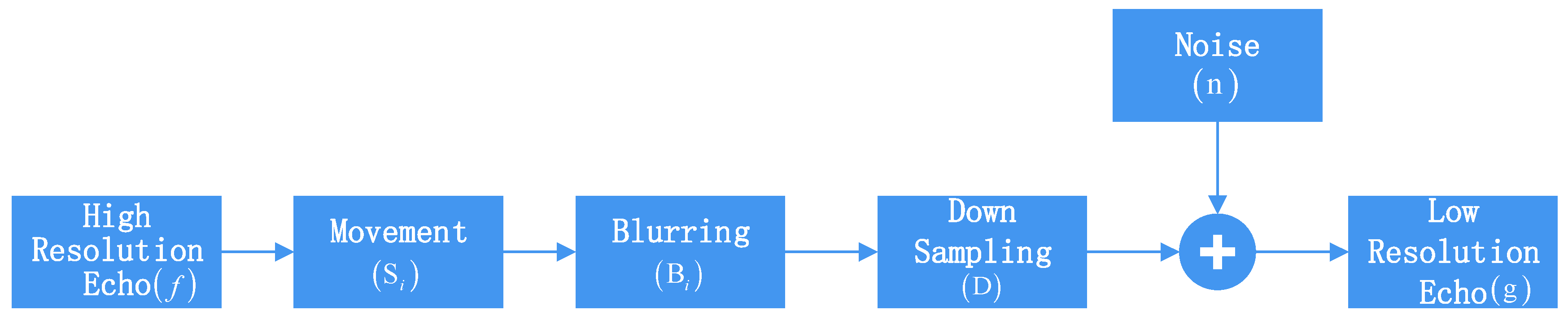
2.1. Super-Resolution Observation Model

The degradation of weather radar echo quality is mainly due to the expansion of the radar antenna beam at a long distance and the combination of blurring, deformation, shifting, and other factors produced by the receiver. The Low-Resolution (LR) observation model is shown in Figure 1.

The observed low-resolution echo, $g$, is a degraded (moved and blurred and down-sampled) version of the high-resolution echo, $f$. The degradation process can be expressed by:

$$g=S_i{B}_{i}Df+n.$$

(1)

In the echo acquisition process, there is motion between the acquired low-resolution echoes due to atmospheric disturbances and the influence of radar receiver rotation. Here, $S_i$ is a shifting operator, and $B_i$ represents a blurring filter, while $D$ is a sampling operator. The additional variable, $n$, denotes the weather radar receiver noise, assuming $n$ conforms to the Gaussian distribution of zero means. For convenience, we call $T=S_i{B}_{i}D$ a degrading operator, $T$ is a composite operator of moving, blurring, and down-sampling. Equation (1) can be generally formulated by:

$$g=Tf+n.$$

(2)

For Equation (2), super-resolution (SR) reconstruction of the radar echo refers to the reconstruction of the high-resolution echo, $f$, with the low-resolution echo, $g$. The reconstruction process is the reverse process of the LR observation model, as shown in Figure 2.

However, the output high-resolution data is very sensitive to the input low-resolution data in super-resolution reconstruction, because a slight change in the input data, such as the noise, receiver offset, etc., would cause large fluctuations in the output high-resolution echo. The weather radar echo degradation model is irreversible and cannot be accurately estimated. The reconstruction process as shown in Figure 2 can convert to solve an ill-posed problem. In the past decades, various regularization methods were proposed to address the ill-posed problem, such as [15,16,17,18,19]. Quadratic Tikhonov regularization [15] and TV regularization [16,18,19,20] are effective in reconstructing radar echo, but the classic regularization algorithm tends to over smooth the details of radar echo. In recent years, sparsity-based regularization [17,21,22,23,24,25] was proposed and has achieved promising results. The sparsity-based regularization algorithm is suitable for weather radar echo data super-resolution reconstruction because weather radar echo data has better sparsity than normal data, such as images and videos.

2.2. Sparse Representation of Radar Echo

The weather radar collects and records weather data in a unit of files. For different types of radar, the format of files is different. For the CINRAD-SA radar, a data file includes a volume scan header and volume data records. The volume scan data records usually contain a lot of missing data range bins. The missing data range bins refer to data that were sampled beyond the threshold for 8-bit reflectivity level codes or when the corresponding range bin is in an area of the atmosphere that weather does not exist in [26]. Figure 3 shows the proportion histogram of the missing data of level-II radar data products in raw data. $Z_{SA}$ and $V_{SA}$ represent the reflectivity data and velocity data of the CINRAD-SA radar. $Z$, $Z_{dr}$, and $\rho$ denote the reflectivity, differential reflectivity, and correlation coefficient of the X-band dual-polarization radar (XPRAD) [27]. We chose the rainfall XPRAD data and tornado CINRAD-SA data as our test data. It can be seen that the missing data occupies a large proportion of the raw data in Figure 3. Because of the existence of a large amount of missing data, the weather radar data has better sparsity than the image data. The reconstruction method based on sparse representation would achieve better performance in data that is more sparse [28]. In this paper, sparsity-based regularization was adopted to reconstruct radar echo.

For Equation (2), the sparse representation model assumes that $f\in {ℝ}^n$ can be represented as $f\approx D\alpha$, where $D\in {ℝ}^{n\times K}$ is an over-complete dictionary, where $\alpha \in {ℝ}^K$ is a vector with very few ($\ll K$) nonzero entries. The representation of $f$ over $D$ can be obtained from its observation, $g$, by solving an $l_0$-minimization problem, formulated as ${\alpha }_f=\arg {\min }_{\alpha }{\Vert \alpha \Vert }_0$, $s.t.{\Vert f-D\alpha \Vert }_2\le \epsilon$, where the $l_0$-norm counts the number of nonzero coefficients in vector $\alpha$, and $\epsilon$ is a small constant controlling the approximation error. Since the $l_0$-minimization is an Non-deterministic Polynomial (NP)-hard combinatorial search problem, and we often use the $l_1$-minimization, as the closest convex function to $l_0$-minimization, as an alternative approach to solve the sparse coding problem, as follows:

$${\alpha }_f=\arg \underset{\alpha }{\min }\left\{{\Vert f-D\alpha \Vert }_2^2+\lambda {\Vert \alpha \Vert }_1\right\},$$

(3)

where the constant, $\lambda$, denotes the regularization parameter that is used to adjust the convergence speed of the algorithm. To solve Equation (3), many algorithms have been proposed, such as iterative thresholding algorithms [17,29] and Bregman split algorithms [30,31].

For Equation (2), to recover high-resolution radar echo, $f$, from low-resolution radar echo, $g$, first, we can acquire the sparse representation vector, ${\alpha }_g$, of $g$ with respect to $D$ by solving the following problem:

$${\alpha }_g=\arg \underset{\alpha }{\min }\left\{{\Vert g-TD\alpha \Vert }_2^2+\lambda {\Vert \alpha \Vert }_1\right\}.$$

(4)

Then, $f$ is reconstructed by $\widehat{f}=D{\alpha }_g$, where $\widehat{f}$ denotes the reconstructed high-resolution radar echo.

More precisely, for a low-resolution radar echo, $g\in {ℝ}^N$, we can obtain a low-resolution radar echo patch of size $\sqrt{n}\times \sqrt{n}$ at location $i$, which is denoted as $g_i=P_{i}g$, where $P_i$ is the matrix getting patch, $g_i$, at location $i$. With an over-complete dictionary, $D\in {ℝ}^{n\times M},n\le M$, each patch can be sparsely represented as $g_i\approx D{\alpha }_{g,i}$, by solving an $l_1$-minimization problem:

$${\alpha }_{g,i}=\arg \underset{{\alpha }_i}{\min }\left\{{\Vert g_i-D{\alpha }_i\Vert }_2^2+\lambda {\Vert {\alpha }_i\Vert }_1\right\}.$$

(5)

Then, we can obtain the set of sparse code, $\left\{{\alpha }_{g,i}\right\}$. However, reconstructing high-resolution radar echo from $\left\{{\alpha }_{g,i}\right\}$ is an over-determined system, and a straightforward least-square solution is adapted to fix that [21]. For convenience, we let:

$$\widehat{f}\approx D\circ {\alpha }_g={\left({\displaystyle {\sum }_{i=1}^N{P}_i^T{P}_i}\right)}^{-1}{\displaystyle {\sum }_{i=1}^N\left(P_i^{T}D{\alpha }_{g,i}\right)},$$

(6)

where ${\alpha }_g$ denotes the concatenation of all ${\alpha }_{g,i}$. For Equation (4), we can express this as follows:

$${\alpha }_g=\arg \underset{\alpha }{\min }\left\{{\Vert g-TD\circ \alpha \Vert }_2^2+\lambda {\Vert \alpha \Vert }_1\right\}.$$

(7)

Then, the high-resolution radar echo, $f$, is reconstructed by $\widehat{f}=D\circ {\alpha }_g$.

3. Nonlocal Self-Similarity Sparse Representation (NSSR)

The sparse code of low-resolution radar echo should be as close as possible to the sparse code of high-resolution radar echo in order to ideally reconstruct high-resolution radar echo. However, it is difficult to obtain the sparse code of the high-resolution radar echo from the observed radar echo due to the degradation process during observation. In this paper, the sparse coding noise [24] was adapted to describe the difference between the sparse code of low-resolution radar echo and the sparse code of high-resolution radar echo. Although the high-resolution radar echo cannot be directly obtained, the sparse code of high-resolution radar echo can be estimated by using the spatial redundancy in the observed low-resolution radar echo. A set of sub-dictionaries can be learned by training from the observed low-resolution radar echo, and the set of sub-dictionaries are adaptively used to code the radar echo patch that needs to code. Hence, the proposed NSSR model is as follows:

$${\alpha }_g=\arg \underset{\alpha }{\min }\left\{{\Vert g-TD\circ \alpha \Vert }_2^2+\lambda {\displaystyle \sum _i{\Vert {\alpha }_i-{\beta }_i\Vert }_1}\right\}.$$

(8)

Compared with Equation (7), the regularization term in Equation (8) is replaced with NSSR sparse coding noise. $D=\left\{D_k|k=1\cdots K\right\}$ is the concatenation of all sub-dictionaries of the observed radar echo, $\lambda$ is the regularization parameter, ${\alpha }_i$ is the sparse coding vector for each radar echo patch, ${\beta }_i$ is the estimation of ${\alpha }_i$, and $\alpha$ is the concatenation of all ${\alpha }_i$. For Equation (8), one key procedure is the determination of $D$ and we attempt to recover high-resolution radar echo based on the nonlocal self-similarity [32] of the observed low-resolution radar echo. So, we need to learn a series of sub-dictionaries to code the observed radar echo structures. At first, we extracted radar echo patches with size $\sqrt{n}\times \sqrt{n}$ from the observed radar echo. Then, the patch will be involved in dictionary learning if its intensity variance exceeds the threshold, and the purpose of this process is to exclude the invalid data from the observed radar echo and guarantee that the useful patches are involved in dictionary learning.

For a radar echo patch to be coded, the most relevant sub-dictionary will be adaptively selected to code it. To this end, the radar echo patches were selected by the observed echo that should be clustered in $K$ clusters by using the $K$-means clustering method, and learn a sub-dictionary from each of the $K$ clusters. Since the radar echo contains a lot of edge information, the feature for clustering is represented by the high-pass filtering output of each radar echo. For each cluster, there are $n$ numbers of radar echo patches and the principal component analysis (PCA) is applied for each cluster to learn a compact sub-dictionary. So far, we can get $K$ sub-dictionaries, $D_k$, by applying the above procedures to all the $K$ clusters, and adaptively assign a sub-dictionary to each local radar echo patch of $f$ by solving Equation (9), as follows:

$$k_i=\arg \min {\Vert D_c{\widehat{f}}_i-D_c{\mu }_k\Vert }_2,$$

(9)

where ${\mu }_k$ denotes the centroid of the clusters, $D_c$ is the projection matrix composed by the first several most significant eigenvectors, and ${\widehat{f}}_i$ denotes the high-pass filtered radar echo patch. Since the radar echo, $f$, is unknown beforehand, we need to have an initial estimation of it by solving Equation (7). The $k_i{}^{\mathrm{th}}$ sub-dictionary, $D_{k_i}$, will be selected and assigned to the radar echo patch, ${\widehat{f}}_i$, by using Equation (9).

For Equation (8), how to obtain a good estimation, ${\beta }_i$, of ${\alpha }_i$ is a key step in the model solution. Considering the spatial redundancy of the radar echo data, the estimated $\beta$ is learned from the observed radar echo. Let $p_i$ denote the radar echo patch at location $i$ in the observed radar echo. For each local radar patch, $p_i$, radar echo patch redundancy is utilized by searching for the nonlocal similar patches to the given patch in a large window centered at the given radar patch, $p_i$, as Figure 4 shows.

Then, each echo patch, $p_i$, has a set of its similar patches that is denoted by ${\mathsf{\Omega }}_i$. Finally, the optimal estimation, ${\beta }_i$, of ${\alpha }_i$ can be obtained from the sparse codes of the radar echo patches within ${\mathsf{\Omega }}_i$. More specifically, ${\alpha }_{i,q}$ denotes the sparse codes of the radar echo patch, $p_{i,q}$, within set ${\mathsf{\Omega }}_i$, then ${\beta }_i$ can be computed as the weighted average of $p_{i,q}$, as follows:

$${\beta }_i={\displaystyle \sum _{q\in {\mathsf{\Omega }}_i}{\omega }_{i,q}{\alpha }_{i,q}},$$

(10)

where ${\omega }_{i,q}$ is the weight vector. The weight parameters are inversely proportional to the distance between the radar echo patches, $p_i$ and $p_{i,q}$, as follows:

$${\omega }_{i,q}=\frac{1}{W}\exp \left(-{\Vert {\widehat{p}}_i-{\widehat{p}}_{i,q}\Vert }_2^2/h\right).$$

(11)

Here, ${\widehat{p}}_i=D{\widehat{\alpha }}_i$ and ${\widehat{p}}_{i,q}=D{\widehat{\alpha }}_{i,q}$ are the estimation of the radar echo patches, $p_i$ and $p_{i,q}$; $h$ is a pre-determined scalar; and $W$ is the normalization factor. The sparse codes, ${\widehat{\alpha }}_i$ and ${\widehat{\alpha }}_{i,q}$, can be calculated by ${\widehat{\alpha }}_i=D^T{\widehat{p}}_i$ and ${\widehat{\alpha }}_{i,q}=D^T{\widehat{p}}_{i,q}$. The flow of the NSSR algorithm is shown in the following

Table 1. The flow of the nonlocal self-similarity sparse representation (NSSR) algorithm.

Proposed Nonlocal Self-Similarity Sparse Representation (NSSR) Algorithm

1. Initialization: Set the initial estimation, $\widehat{f}$, and initial regularization parameter, $\lambda$. 2. Outer loop: Dictionary learning and parameter estimation. Iterate on $l=1,2,\cdots ,L$: (a) Update the dictionaries $\left\{D_k\right\}$. (b) Inner loop: reconstruct radar echo. Iterate on $k=1,2,\cdots ,K$. (I) Initialize ${\beta }_i^{(-1)}=0$. (II) Compute $f^{(0)}=D\circ {\alpha }_g^{(0)}$. (III) Each radar echo patch, $P_i$, computes the nonlocal estimation, ${\beta }_i^{(0)}$, using Equations (9) and (10). (IV) Repeat the above three steps until its convergence in the $l^{\mathrm{th}}$ iteration. Compute ${\alpha }_g^{(l)}$ using Equation (8). (V) Radar echo estimate update: ${\widehat{f}}^{(l)}=D\circ {\alpha }_g^{(l)}$ using Equation (6). 3. Results: Output the reconstructed HR radar echo, $f$.

.

In NSSR algorithm, we use the bicubic interpolation of the low-resolution radar echo as an initial estimation of the high-resolution radar echo. NSSR algorithm is empirically convergent in general, such as those presented in [33].

4. Experiments

The radar echo super-resolution reconstruction performance of the proposed NSSR algorithm was tested by the level-II weather radar data from China Meteorological Administration. Various weather phenomena were also selected to verify the universality of the algorithm for complex weather conditions.

The rainfall data of XPRAD radar in the South China Heavy Rainfall Observation Experiment and the tornado data of the CINRAD SA radar in Guangzhou were selected as the tested data. Since the weather radar echo degradation model, as shown in Figure 1, is irreversible and cannot be accurately estimated and the point spread functions of different imaging systems are different, so, Gaussian noise is usually used to simulate the process of the degradation of radar echo [7,13,23,24,32,34]. The degraded radar echoes were generated by applying a $7\times 7$ Gaussian kernel of a standard deviation of 1.5 to the high-resolution radar echo and then down-sampled the blurred radar echo by a scaling factor 2 and 4 in both the horizontal and vertical directions. Additionally, the parameter initialization of NSSR was as follows: The number of the PCA sub-dictionary is $K=64$, the regularization parameter is $\lambda =7$. We compared the proposed NSSR approach with the bicubic interpolation and the iterative back-projection algorithm [13].

For level-II CINRAD SA data, we adopted the reflectivity and mean radial velocity data as the tested data. The reflectivity data product contains 11 elevation cuts, and each elevation cut includes 360 radials with 460 range bins per radial direction. The distance resolution of the data is 1 km. The mean radial velocity data format is slightly different from the reflectivity data format, as every mean radial velocity data product has 920 range bins for each of the 360 radials in an elevation cut, and the distance resolution is 0.25 km. For XPRAD data, the reflectivity, differential reflectivity, and correlation coefficient data were selected as the tested data. The XPRAD data products contain 14 elevation cuts, and each elevation cut includes 360 radials with 4000 range bins per radial direction. The distance resolution of the data is 0.075 km. We used the top 600 range bins as our experimental data, because the stronger rainfall attenuation in the X-band results in lower data availability from the radar.

The experiment used the original echo data as high-resolution echo data. First, the original echo data was blurred and down-sampled to obtain simulated low-resolution echo data. Additionally, the bicubic interpolation results of the low-resolution echo data were used as the input of the proposed algorithm. Super-resolution reconstruction of the low-resolution echo data was then performed using different algorithms. Finally, the subjective visual quality and objective evaluation of the high-resolution echo data and super-resolution reconstructed echo data were compared. Objective evaluation criteria included: PSNR (peak signal to noise ratio) describing the reconstruction quality and SSIM (structural similarity index) describing the structural similarity.

CINARAD SA data (the tested data is the first elevation cut of the CINRAD SA radar at 11:24 (BJT) on 18 August 2018, Tornado, Xuzhou City, Jiangsu, China) was used to test the effectiveness of the algorithm for CINARAD data. Reflectivity and mean radial velocity data were selected as the test data. The visual comparison of the radar echo reconstruction methods and their corresponding original level-II CINARAD SA data products’ PPI are presented in Figure 5 and Figure 6. From Figure 5, we can see that the bicubic interpolation tends to over-smooth the reconstructed radar echo, resulting in the partial loss of the red strong echo information in the black square in Figure 5a, while both IBP [13] and NSSR can reconstruct most of the red strong echo information. The reconstructed echoes by NSSR are more similar to the original radar echo than that reconstructed by IBP [13], especially in radar echo edges and detailed information. Figure 6 represents the mean radial velocity PPI of the tornado CINRAD SA data, and the purple area in the black rectangle represents the center of the tornado. As can be seen from Figure 6a, the velocity PPI reconstructed by NSSR can better restore the details of the tornado center, while the other methods cannot reconstruct the tornado center in the radar echo. According to Figure 5 and Figure 6, the NSSR algorithm has a good effect on the super-resolution reconstruction of CINRAD SA data. In order to verify whether the NSSR is universal for adaption to different weather phenomena, five groups of severe convective weather, rainfall event, and sunny day CINARAD SA data were selected, respectively, and the reconstructed radar echo was compared with the original high-resolution radar echo. The PSNR and SSIM results are shown in

Table 2. Average PSNR (dB) and SSIM results of the reconstructed echo of five groups of level-II CINRAD SA data.

Level-II Radar Data Products (2×)	Severe Weather			Rainfall			Sun Day
	Bicubic	IBP	NSSR	Bicubic	IBP	NSSR	Bicubic	IBP	NSSR
Reflectivity	32.996	35.055	37.123	31.669	34.141	35.750	33.817	35.228	36.353
	0.8933	0.9500	0.9598	0.8450	0.9284	0.9441	0.9098	0.9421	0.9552
Velocity	27.911	29.459	30.169	26.999	28.916	30.562	29.194	30.025	32.343
	0.8287	0.8937	0.9056	0.8465	0.8948	0.9209	0.8572	0.9179	0.9345

and

Table 3. Average PSNR (dB) and SSIM results of the reconstructed echo of five groups of level-II CINRAD SA data.

Level-II Radar Data Products (4×)	Severe Weather			Rainfall			Sun Day
	Bicubic	IBP	NSSR	Bicubic	IBP	NSSR	Bicubic	IBP	NSSR
Reflectivity	30.588	30.694	33.411	30.244	31.213	32.486	33.817	35.228	36.353
	0.8412	0.8699	0.9031	0.8241	0.8356	0.8978	0.9098	0.9421	0.9552
Velocity	26.921	26.883	28.415	26.332	26.127	28.179	29.194	30.025	32.343
	0.7546	0.8324	0.8501	0.7231	0.8035	0.8471	0.8572	0.9179	0.9345

. From Table 2 and Table 3, we can see that the proposed NSSR algorithm achieves the highest PSNR and SSIM against the other algorithms, and the experimental results show that the NSSR algorithm has good adaptability to various weathers. From the experiments on the CINRAD SA data, we can see that the effect of the reflectivity super-resolution reconstruction is better than the velocity, because the NSSR algorithm is based on the sparsity of the radar data and the reflectivity data is more sparse than the velocity data.

To verify that the NSSR algorithm is also applicable to dual-polarization weather radar data, the reflectivity, differential reflectivity, and correlation coefficient data were selected as the tested data (the tested data is the first elevation cut of the XPRAD at 10:43 (BJT) on 28 May 2016, rainfall event, Xinfeng County, Guangdong Province, China). The visual comparison of the radar echo reconstruction methods and their corresponding original level-II XPRAD data products’ PPI are presented in Figure 7, Figure 8 and Figure 9. From Figure 7, Figure 8 and Figure 9, we can see that the NSSR can also apply to XPRAD data: The reconstructed XPRAD echo by NSSR can better restore the details and edges than IBP [13]. Similarly, to verify whether the NSSR is universal for adaption to different weather phenomena, five groups of severe convective weather, rainfall event, and sunny day XPRAD data were selected, respectively, and the reconstructed radar echo was compared with the original high-resolution radar echo. The PSNR and SSIM results are shown in

Table 4. Average PSNR (dB) and SSIM results of the reconstructed echo of five groups of level-II XPRAD data.

Level-II Radar Data Products (2×)	Severe Weather			Rainfall			Sun Day
	Bicubic	IBP	NSSR	Bicubic	IBP	NSSR	Bicubic	IBP	NSSR
Reflectivity	35.362	38.798	40.809	35.691	38.038	40.557	37.188	38.524	41.807
	0.9338	0.9823	0.9844	0.9393	0.9789	0.9843	0.9598	0.9843	0.9989
Differential Reflectivity	51.007	52.840	55.621	46.910	48.501	50.410	46.860	48.822	50.635
	0.9891	0.9935	0.9975	0.9821	0.9835	0.9942	0.9851	0.9853	0.9947
Correlation Coefficient	67.436	70.223	72.121	67.936	70.404	72.029	70.080	72.246	74.542
	0.9996	0.9998	0.9999	0.9996	0.9997	0.9999	0.9998	0.9998	0.9999

and

Table 5. Average PSNR (dB) and SSIM results of the reconstructed echo of five groups of level-II XPRAD data.

Level-II Radar Data Products (4×)	Severe Weather			Rainfall			Sun Day
	Bicubic	IBP	NSSR	Bicubic	IBP	NSSR	Bicubic	IBP	NSSR
Reflectivity	32.294	32.458	35.525	32.883	32.454	36.140	34.531	33.325	37.698
	0.8834	0.9113	0.9446	0.8966	0.9185	0.9519	0.9348	0.9461	0.9689
Differential Reflectivity	48.479	48.562	50.156	45.055	45.128	47.124	45.627	45.500	47.130
	0.9816	0.9876	0.9924	0.9654	0.9727	0.9831	0.9741	0.9779	0.9855
Correlation Coefficient	64.571	65.487	67.102	65.799	66.175	68.058	65.794	68.315	70.231
	0.9988	0.9992	0.9996	0.9986	0.9993	0.9998	0.9990	0.9996	0.9998

. From Table 4 and Table 5, we can see that the proposed NSSR algorithm achieves the highest PSNR and SSIM against the other algorithms. The experimental results show that the NSSR algorithm has good adaptability to various weather events. Although the differential reflectivity and correlation coefficient data achieved the highest PSNR and SSIM in radar echo reconstruction, the visual quality was not very good compared with original echo and other reconstructed level-II radar data products. The reason is the range of the differential reflectivity and correlation coefficient data is small and, especially on rainy days, most correlation coefficients are close to 1. From Figure 3, we can see that the XPRAD data is more sparse than the CINARAD SA data, so, the PSNR and SSIM results of the reconstructed XPRAD echo by NSSR are better than that of the CINARAD SA.

5. Conclusions

These results prove the outstanding performance of NSSR for level-II weather radar data super-resolution reconstruction. The NSSR model is suitable for super-resolution reconstruction of both CINRAD radar data and dual-polarized weather radar data products. In particular, the model has excellent reconstruction effects on the edge and structural details of weather radar echoes. The NSSR method can be applied to enhance the resolution of weather radars and space-time integration of networked observations at different frequencies.

Weather radar data is different from image or video data. Since spatial target distribution tends to be concentrated in a certain area, meteorological radar data is sparser than image data. The better sparsity makes the reconstruction of the structure and edge information of the reconstruction results more precise. Most of the super-resolution reconstruction algorithms use an iterative algorithm with a large amount of computation. Excessive computational complexity is an important factor that constrains the application of its super-resolution algorithms. We compared the time taken by NSSR and IBP [13] to super-resolution reconstruct the same radar echo under the same environment. Five groups of strong convective weather, rainfall event, and sunny day CINARAD SA data and XPRAD data were selected, respectively. The experimental results showed that NSSR spends more time than IBP [13], and the NSSR algorithm need to be further optimized to meet the needs of real-time applications. According to different application requirements, the design of the corresponding super-resolution reconstruction algorithm still requires a lot of work.

References

1. Peleg, N.; Marra, F.; Fatichi, S.; Molnar, P.; Morin, E.; Sharma, A.; Burlando, P. Intensification of convective rain cells at warmer temperatures observed from high-resolution weather radar data. J. Hydrometeorol. 2018, 19, 715–726. [Google Scholar] [CrossRef]
2. Kendon, E.J.; Roberts, N.M.; Fowler, H.J.; Roberts, M.J.; Chan, S.C.; Senior, C.A. Heavier summer downpours with climate change revealed by weather forecast resolution model. Nat. Clim. Chang. 2014, 4, 570. [Google Scholar] [CrossRef]
3. Herman, M.A.; Strohmer, T. High-resolution radar via compressed sensing. IEEE Trans. Signal Process. 2009, 57, 2275–2284. [Google Scholar] [CrossRef]
4. Kumjian, M.R.; Ryzhkov, A.V.; Melnikov, V.M.; Schuur, T.J. Rapid-scan super-resolution observations of a cyclic supercell with a dual-polarization WSR-88D. Mon. Weather Rev. 2010, 138, 3762–3786. [Google Scholar] [CrossRef]
5. Borowska, L.; Zhang, G.; Zrnić, D.S. Considerations for oversampling in azimuth on the phased array weather radar. J. Atmos. Ocean. Technol. 2015, 32, 1614–1629. [Google Scholar] [CrossRef]
6. Torres, S.M.; Curtis, C.D.; Technology, O. The Impact of Range-Oversampling Processing on Tornado Velocity Signatures Obtained from WSR-88D Superresolution Data. J. Atmos. Ocean. Technol. 2015, 32, 1581–1592. [Google Scholar] [CrossRef]
7. Li, X.; He, J.; He, Z.; Zeng, Q. Weather radar range and angular super-resolution reconstruction technique on oversampled reflectivity data. J. Inf. Comput. Sci. 2011, 8, 2553–2562. [Google Scholar]
8. Zha, Y.; Liu, L.; Yang, J.; Huang, Y. An alternating direction method for angular super-resolution in scanning radar. In Proceedings of the 2017 IEEE International Geoscience and Remote Sensing Symposium (IGARSS), Fort Worth, TX, USA, 23–28 July 2017; pp. 1626–1629. [Google Scholar]
9. Wu, Y.; Zhang, Y.; Zhang, Y.; Huang, Y.; Yang, J. TSVD with least squares optimization for scanning radar angular super-resolution. In Proceedings of the 2017 IEEE Radar Conference (RadarConf), Seattle, WA, USA, 8–12 May 2017; pp. 1450–1454. [Google Scholar]
10. Tan, K.; Li, W.; Zhang, Q.; Huang, Y.; Wu, J.; Yang, J. Penalized Maximum Likelihood Angular Super-Resolution Method for Scanning Radar Forward-Looking Imaging. Sensors 2018, 18, 912. [Google Scholar] [CrossRef]
11. Mao, D.; Zhang, Y.; Zhang, Y.; Huang, Y.; Yang, J. Realization of airborne forward-looking radar super-resolution algorithm based on GPU frame. In Proceedings of the 2016 CIE International Conference on Radar (RADAR), Guangzhou, China, 10–13 October 2016; pp. 1–5. [Google Scholar]
12. Zeng, Q.; He, J.; Shi, Z.; Li, X. Weather Radar Data Compression Based on Spatial and Temporal Prediction. Atmosphere 2018, 9, 96. [Google Scholar] [CrossRef]
13. He, J.; Ren, H.; Zeng, Q.; Li, X. Super-Resolution reconstruction algorithm of weather radar based on IBP. J. Sichuan Univ. (Nat. Sci. Ed.) 2014, 51, 415–418. [Google Scholar]
14. Narayanan, S.; Sahoo, S.K.; Makur, A. Sparse recovery of radar echo signals using Adaptive Backtracking Matching Pursuit. In Proceedings of the 2015 IEEE Radar Conference, Johannesburg, South Africa, 27–30 October 2015; pp. 339–343. [Google Scholar]
15. Tihonov, A.N. Solution of incorrectly formulated problems and the regularization method. Sov. Math 1963, 4, 1035–1038. [Google Scholar]
16. Rudin, L.I.; Osher, S.; Fatemi, E. Nonlinear total variation based noise removal algorithms. Phys. D Nonlinear Phenom. 1992, 60, 259–268. [Google Scholar] [CrossRef]
17. Daubechies, I.; Defrise, M.; De Mol, C. An iterative thresholding algorithm for linear inverse problems with a sparsity constraint. Commun. Pure Appl. Math. J. Issued Courant Inst. Math. Sci. 2004, 57, 1413–1457. [Google Scholar] [CrossRef] [Green Version]
18. Chan, T.; Esedoglu, S.; Park, F.; Yip, A. Recent developments in total variation image restoration. Math. Models Comput. Vis. 2005, 17–30. [Google Scholar]
19. Oliveira, J.P.; Bioucas-Dias, J.M.; Figueiredo, M.A. Adaptive total variation image deblurring: A majorization–minimization approach. Signal Process. 2009, 89, 1683–1693. [Google Scholar] [CrossRef]
20. He, J.; Ren, H.; Zeng, Q.; Li, X. Super-resolution Reconstruction of Weather Radar Echo Based on the Improved Total Variation. Comput. Simul. 2014, 31, 415–418. [Google Scholar]
21. Michael, E.; Michal, A. Image denoising via sparse and redundant representations over learned dictionaries. IEEE Trans. Image Process. 2006, 15, 3736–3745. [Google Scholar]
22. Mairal, J.; Bach, F.; Ponce, J.; Sapiro, G.; Zisserman, A. Non-local sparse models for image restoration. In Proceedings of the 2009 IEEE 12th International Conference on Computer Vision (ICCV), Kyoto, Japan, 29 September–2 October 2009; pp. 2272–2279. [Google Scholar]
23. Weisheng, D.; Lei, Z.; Guangming, S.; Xiaolin, W. Image deblurring and super-resolution by adaptive sparse domain selection and adaptive regularization. IEEE Trans. Image Process. 2011, 20, 1838–1857. [Google Scholar] [CrossRef]
24. Dong, W.; Zhang, L.; Shi, G.; Li, X. Nonlocally centralized sparse representation for image restoration. IEEE Trans. Image Process. 2013, 22, 1620–1630. [Google Scholar] [CrossRef]
25. Zhang, J.; Zhao, D.; Gao, W. Group-based sparse representation for image restoration. IEEE Trans. Image Process. 2014, 23, 3336–3351. [Google Scholar] [CrossRef]
26. Mccarroll, S.; Yeary, M.; Hougen, D.; Lakshmanan, V.; Smith, S. Approaches for Compression of Super-Resolution WSR-88D Data. IEEE Geosci. Remote Sens. Lett. 2011, 8, 191–195. [Google Scholar] [CrossRef]
27. Shi, Z.; Chen, H.; Chandrasekar, V.; He, J. Deployment and performance of an X-band dual-polarization radar during the Southern China Monsoon Rainfall Experiment. Atmosphere 2017, 9, 4. [Google Scholar] [CrossRef]
28. Mallat, S.G.; Zhang, Z. Matching pursuits with time-frequency dictionaries. IEEE Trans. Signal Process. 1993, 41, 3397–3415. [Google Scholar] [CrossRef] [Green Version]
29. Zibulevsky, M.; Elad, M. L1-L2 Optimization in Signal and Image Processing. IEEE Signal Process. Mag. 2010, 27, 76–88. [Google Scholar] [CrossRef]
30. Marquina, A.; Osher, S.J. Image super-resolution by TV-regularization and Bregman iteration. J. Sci. Comput. 2008, 37, 367–382. [Google Scholar] [CrossRef]
31. Zhang, X.; Burger, M.; Bresson, X.; Osher, S. Bregmanized nonlocal regularization for deconvolution and sparse reconstruction. SIAM J. Imaging Sci. 2010, 3, 253–276. [Google Scholar] [CrossRef]
32. Glasner, D.; Bagon, S.; Irani, M. Super-resolution from a single image. In Proceedings of the 2009 IEEE 12th International Conference on Computer Vision (ICCV), Kyoto, Japan, 29 September–2 October 2009; pp. 349–356. [Google Scholar]
33. Candes, E.J.; Wakin, M.B.; Boyd, S.P. Enhancing sparsity by reweighted ℓ 1 minimization. J. Fourier Anal. Appl. 2008, 14, 877–905. [Google Scholar] [CrossRef]
34. Tipping, M.E.; Bishop, C.M. Bayesian image super-resolution. In Proceedings of the 2003 Advances in neural information processing systems, Vancouver, BC, Canada, 8–13 December 2003; pp. 1303–1310. [Google Scholar]
Figure 1. Low resolution observation model.
Atmosphere 10 00254 g001
Figure 2. Reconstruction process.
Atmosphere 10 00254 g002
Figure 3. The proportion histogram of the missing data of level-II radar data products in raw data. The CINRAD SA reflectivity data is the first elevation cut of the radar at 11:24 (BJT) on 18 August 2018, and the CINRAD SA velocity data corresponding to reflectivity is the second elevation cut of the radar. The X-band dual-polarization radar (XPRAD) data is the first elevation cut of the radar at 10:43 (BJT) on 28 May 2016.
Atmosphere 10 00254 g003
Figure 4. An example of searching for the nonlocal similar patches to the given radar echo patch. The black square in the left Plan Position Indicator (PPI) represents the given patch which needs to search the nonlocal similar patches. The big square in the right PPI represents the search window, the red square represents the given patch, and the other squares in the right PPI represent the similar patches to the given patch using the moving window model within the search window. The tested data is the first elevation cut of the CINRAD SA radar on 23 September 2008 at 20:13 (BJT), which has 360 radials in an elevation cut. Each radial has 460 range bins.
Atmosphere 10 00254 g004
Figure 5. Radar echo reconstruction comparison on reflectivity data. (a) 2 × reconstruction of reflectivity data. From left to right and top to bottom: bicubic interpolation echo, the reconstructed echo by IBP [13] (PSNR = 35.3572; SSIM = 0.9556), original radar echo, and the reconstructed echo by the proposed NSSR algorithm (PSNR = 37.3138; SSIM = 0.9609). (b) 4 × reconstruction of reflectivity data. From left to right and top to bottom: LR radar echo, the reconstructed echo by IBP [13] (PSNR = 30.5857; SSIM = 0.8656), original radar echo, and the reconstructed echo by the proposed NSSR algorithm (PSNR = 33.5267; SSIM = 0.9062). The tested data is the first elevation cut of the CINRAD SA radar at 11:24 (BJT) on 18 August 2018.
Atmosphere 10 00254 g005aAtmosphere 10 00254 g005b
Figure 6. Radar echo reconstruction comparison on radial velocity data. (a) 2 × reconstruction of radial velocity data. From left to right and top to bottom: bicubic interpolation echo, the reconstructed echo by IBP [13] (PSNR = 30.0435; SSIM = 0.9184), original radar echo, and the reconstructed echo by the proposed NSSR algorithm (PSNR = 31.1579; SSIM = 0.9253). (b) 4 × reconstruction of reflectivity data. From left to right and top to bottom: bicubic interpolation echo, the reconstructed echo by IBP [13] (PSNR = 26.8634; SSIM = 0.8303), original radar echo, and the reconstructed echo by the proposed NSSR algorithm (PSNR = 28.4852; SSIM = 0.8524). The tested data is the second elevation cut of the CINRAD SA radar, which is the same as the data used in Figure 5.
Atmosphere 10 00254 g006
Figure 7. Radar echo reconstruction comparison on reflectivity data. (a) 2 × reconstruction of reflectivity data. From left to right and top to bottom: bicubic interpolation echo, the reconstructed echo by IBP [13] (PSNR = 39.1936; SSIM = 0.9867), original radar echo, and the reconstructed echo by the proposed NSSR algorithm (PSNR = 41.9943; SSIM = 0.9877). (b) 4 × reconstruction of reflectivity data. From left to right and top to bottom: bicubic interpolation echo, the reconstructed echo by IBP [13] (PSNR = 32.9533; SSIM = 0.9221), original radar echo, and the reconstructed echo by the proposed NSSR algorithm (PSNR = 37.1748; SSIM = 0.9588). The tested data is the first elevation cut of the XPRAD at 10:43 (BJT) on 28 May 2016.
Atmosphere 10 00254 g007
Figure 8. Radar echo reconstruction comparison on differential reflectivity data. (a) 2 × reconstruction of differential reflectivity data. From left to right and top to bottom: bicubic interpolation echo, the reconstructed echo by IBP [13] (PSNR = 54.6148; SSIM = 0.9971), original radar echo, and the reconstructed echo by the proposed NSSR algorithm (PSNR = 57.1143; SSIM = 0.9983). (b) 4 × reconstruction of differential reflectivity data. From left to right and top to bottom: bicubic interpolation echo, the reconstructed echo by IBP [13] (PSNR = 49.3183; SSIM = 0.9871), original radar echo, and the reconstructed echo by the proposed NSSR algorithm (PSNR = 52.9308; SSIM = 0.9943). The tested data is the first elevation cut of the XPRAD, which is the same as the data used in Figure 7.
Atmosphere 10 00254 g008aAtmosphere 10 00254 g008b
Figure 9. Radar echo reconstruction comparison on correlation coefficient data. (a) 2 × reconstruction of correlation coefficient data. From left to right and top to bottom: bicubic interpolation echo, the reconstructed echo by IBP [13] (PSNR = 71.6387; SSIM = 0.9998), original radar echo, and the reconstructed echo by the proposed NSSR algorithm (PSNR = 73.3858; SSIM = 0.9999). (b) 4 × reconstruction of correlation coefficient data. From left to right and top to bottom: bicubic interpolation echo, the reconstructed echo by IBP [13] (PSNR = 66.7864; SSIM = 0.9994), original radar echo, and the reconstructed echo by the proposed NSSR algorithm (PSNR = 68.8336; SSIM = 0.9998). The tested data is the first elevation cut of the XPRAD, which is the same as the data used in Figure 7.
Atmosphere 10 00254 g009