1. Introduction
In the context of the effective management of crises and disasters, which is a global challenge, the risk of an accident releasing airborne harmful material to the atmosphere, like radioactive, chemical or bacteriological active substances, cannot be ruled out. To face these kinds of events, it is well recognized that good preparedness substantially improves the emergency response. In this line, efforts to promote and enhance global safety, and to limit and mitigate any consequences associated with these kinds of releases are continuously triggered at national and international levels [
1].
The early phase of a harmful release to the atmosphere is a period usually characterized by large uncertainty in the source term release characteristics and the lack of field measurements. Within this period, to have available a prior estimation of the possible atmospheric transport and dispersion of the released material, and hence, the likely areas to be affected by the plume, is of importance to decision makers and emergency managers in an attempt at minimizing its health and environmental impacts.
Meteorological conditions determine the dispersion and transport of substances in the atmosphere. Rainfall, wind speed, wind direction and temperature are relevant parameters in establishing their temporal and spatial variability. Once in the atmosphere, the primary process favoring the transport and dispersion of substances is wind regimes, which is characterized by wind direction and wind speed, e.g., the greater the wind velocity is, then the greater the dispersion of the contaminants, and the lower their concentration is [
2]. Many studies [
3,
4] have outlined the need of characterizing wind regimes to understand air pollution scenarios. This direct link makes the knowledge and characterization of wind regimes at a site become key information in estimating the atmospheric transport and dispersion of harmful substances and, therefore, in forecasting the likely areas affected by the plume passage.
Air trajectory analysis is a central scientific tool to characterize synoptic and regional wind regimes [
5]. The basic methodological approach in this kind of analysis is to generate massive amounts of air mass trajectories with the purpose of considering a large number of transport and dispersion scenarios so that the statistical analysis leads to the extraction of representative information about flow patterns (e.g., residence time, range, distance, speed, etc.). When compiled and studied over multiple years [
6,
7], the outcome of this trajectory analysis is used to generate an estimation of future wind scenarios.
With this in mind, the aim of this paper is to describe and to evaluate a method to estimate the likely areas to be affected by a hypothetical release to the atmosphere. The present methodology, which is based on the influence that lower atmosphere meteorology has on the dispersion and transport of substances in the atmosphere, is based on the calculation of density maps from air mass trajectories by applying the kernel density estimation (KDE) method [
8]. KDE’s strength is its ability to provide an estimate of density at any location in the spatial frame. In this present framework, these density maps report the areas with the longest residence time of air masses, and hence, the areas where the deposit may be substantial. Residence time analysis [
9] identifies the likelihood that an air mass will traverse a given region in its movement to or from the site of interest over a given time period [
7,
10]. The longer the residence time over certain areas is, the more favorable the situation for significant surface dry deposition from contaminant plumes is.
Considering that the calculation of air mass trajectories is purely based on meteorological fields, i.e., we are not considering any release to the atmosphere (source term) in the calculation, we can only address a qualitative comparison to evaluate the outcomes of this method, e.g., between areas of high residence time and high deposit. To estimate the bias of this meteorological approach, we have evaluated it against the period 2006–2017 and two radioactive dispersion events, such as Chernobyl accident and Algeciras release. The corresponding density maps for each case study, which identify those areas with the longest residence time of air masses, are then qualitatively compared with those areas affected by high deposits in each release scenario. Reasonable estimation of the areas affected by both releases would prove the usefulness of this method and the number of years selected in the estimation of likely areas to be affected by a hypothetical release.
While far from being fully comprehensive of the complexity behind the simulation and prediction of atmospheric dispersion, as only meteorological data are used, this method would provide useful guidance in estimating the transport and dispersion that might result if harmful material reaches the atmosphere, and hence, in increasing knowledge of crisis and disaster management for improving responsiveness. Being only based on the analysis of the wind field, this method can be used, for instance, for any kind of airborne material.
The article is structured as followed. In
Section 2, we describe the methodology applied to obtain density maps from air mass end-point positions, while
Section 3 is dedicated to showing and discussing the results obtained in the two study cases taken as reference. To finalize, the conclusions obtained from this work are shown in
Section 4.
2. Materials and Methods
2.1. Trajectory Modelling
Air mass trajectory shows the pathway of an infinitesimal air parcel through a centerline of an advected air mass having vertical and horizontal dispersion [
11]. Forward trajectory estimates the pathway to be followed by an air parcel downwind from the selected coordinates in due course of time.
The National Oceanic and Atmospheric Administration (NOAA) Air Resources Laboratory’s (ARL) Hybrid Single-Particle Lagrangian Integrated Trajectory model (HYSPLIT 4.9) [
12] is used to calculate forward kinematic three-dimensional trajectories. The computation of three-dimensional trajectories is based on the use of the vertical velocity field included in publicly available meteorological datafiles, such as the 3-hourly meteorological archive data from NCEP’s GDAS (National Weather Service’s National Centers for Environmental Prediction-Global Data Assimilation System) [
13]. The GDAS covers from 2004 to the present, which is a big advantage in favor of using them in research studies, as they span 10 years or more. The GDAS is run 4 times a day, i.e., at 0000, 0600, 1200, and 1800 UTC. These data are archived and made available by the NOAA’s ARL as a global and 1-degree latitude–longitude dataset on pressure surface.
Our method uses forward trajectories with duration of 120 hours (length of the trajectory). A complete description of all the equations and HYSPLIT calculation methods for trajectories can be seen in [
14]. HYSPLIT provides the coordinates (longitude and latitude) and height (in meters above ground level, a.g.l) of every trajectory calculated at 1-h intervals. Therefore, each trajectory of 120 h is composed of 120 end-point positions. In our study, we work these 120 end-point positions, which are the position of the lagrangian particles, at a certain hour within the duration of 120 h.
2.2. Kernel Density Estimation
Kernel density estimation (KDE) [
8] is an important method in visualizing and analyzing spatial data, with application in many fields (ecology, public health, etc.), with the objective of understanding and potentially predicting event patterns [
15,
16,
17]. KDE is a non-parametric approach to the estimation of probability density functions using a finite number of cases [
18]. This method compensates for in distance the influence of a case in its vicinity. To this purpose, it incorporates a decay function that assigns smaller values to locations which are still in the neighborhood, but further way from a case [
15]. To achieve this, KDE fits a curved surface over each case such that the surface is highest above the center and zero at a specified distance from the case (the bandwidth, i.e., the distance around a case at which its influence is felt). The influence of a number of cases at a certain location, over a two-dimensional space, can be represented as the following definition [
8,
19]:
where
f(x,y) is the density value at location (x,y), n is the total number of cases under concern,
h is the bandwidth,
di is the geographical distance between case
i and the location and
K is a density function (generally a radially symmetric unimodal probability density function) which integrates to one. Different density functions (
K) can be used, e.g., Cauchy [
20], Epanechnikov [
21], Gaussian [
22]. More information about different kernel-smoothing algorithms can be found in [
23].
The KDE refers to high or low density of points, i.e., cases per unit area. Therefore, KDE method detects the highs and lows of cases densities of the pattern, and is useful for detecting hot spots.
Figure 1 graphically shows an example of the procedure use in our method to determine the density value
f(x,y) (grey squared) over the raster data by considering two cases (red circles).
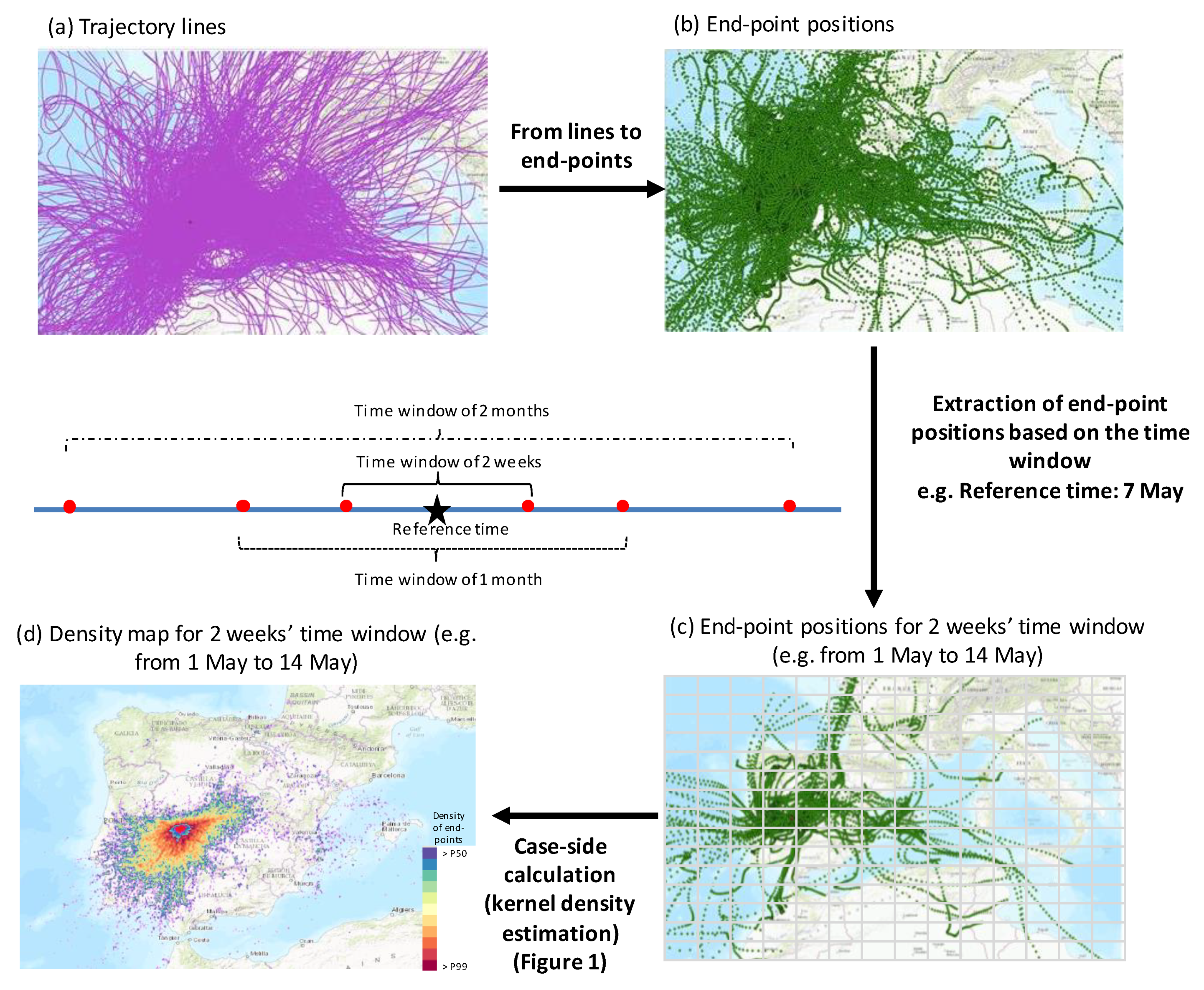
2.3. Method
Figure 2 shows the procedure applied in our method to determine the corresponding density maps. Once calculated, the trajectories for the period 2007–2016 (
Figure 2a), and the corresponding end-point positions (i.e., cases in
Section 2.2), the subset of end-point positions within the analyzed period (hereafter, time window), are extracted (
Figure 2b). We define the “time window” as the reference period for which end-point positions are collected and to which, as a result, the density map refers. This time window refers to one reference time (e.g., a specific day, such as the release date or the maximum concentration date). The definition of the time window is based on the fact of having evidences that cyclicality plays a significant role in the weather we experience, i.e., weather appears to be a regularly cycling pattern over short and long-range time. In the present method, we consider three different temporal cycling patterns of weather, e.g., two weeks, one month and two months. As an example, if the event date is 7 May, we work with all end-point positions within the period 2007–2016 from 1 May to 14 May (one week before and after the release date), from 24 April to 21 May (two weeks before and after), and from 7 April to 7 June (one month before and after).
Based on the end-point positions extracted, we provide a comprehensive analysis of the residence time of air masses. In order to accommodate as much as possible the residence time with hypothetical deposits from the plume, the present analysis is carried out by selecting the number of end-point positions below a vertical level, which is set to 100 m a.g.l., within the selected time window
Once the subset of end-point positions within the time window and with a height less than 100 m a.g.l are selected, these are then displayed as a density map using the KDE method indicated in
Section 2.2 (
Figure 2c,d). To make a KDE, the challenge is to select the kernel function, the bandwidth and the cell size. However, there are no rules and standards concerning this selection, and they are predominantly taken as the results of experimental studies [
24]. After several analyses, in the present work, end-point positions are displayed on a map with a fixed grid cell size of 3 × 3 km and we have defined a bandwidth of 9 km, while the kernel function is based on the quartic kernel function described in [
8], i.e., an inverse distance weighting (
Figure 1). We have used the free and open source QGIS geographic information system [
25].
3. Case Studies
Two case studies, the Chernobyl accident (25–26 April 1986) and the Algeciras release (30 May 1998), have been taken as reference in order to evaluate the use of trajectories and density maps as valuable information in the preparedness phase of an atmospheric event release.
An explosive accident took place at the Chernobyl nuclear power plant unit IV in Ukraine on 25 April 1986 at 2123 UTC. This accident led to a widespread dispersion of radioactive materials released at different times in the atmosphere at a continental scale. The meteorological conditions caused the various plumes to take different directions according to the release date [
26], and therefore, contaminated clouds flew all around the world.
On 30 May, 1998, a 137Cs medical source was accidentally melted in one of the furnaces at the Acerinox stainless steel production plant near Algeciras, southern Spain. An unknown amount of contaminated air was dispersed over the western coast of Spain and travelled all the way north, reaching the southern coast of France and northern Italy two to three days after the release. The International Atomic Energy Agency (IAEA) Emergency Response Centre reported the occurrence of a radiological accident on June 12.
Following the methodology explained in
Section 2.3, we have calculated the forward trajectories and the corresponding end-point positions for the 10-year period (2007–2016) at Chernobyl (51° 23′ 23.47″ N, 30° 5′ 38.57″ E) and Algeciras (6°7′39″ N, 5°27′14″ W).
In accordance with the release characteristic of each release scenario [
27,
28], the initial height applied in the calculation of trajectories differs: Chernobyl at 1000 m a.g.l and Algeciras release at 100 m a.g.l. For each scenario, over 97% of 1-h trajectories in the period 2007–2016 are completed for all 120 h (an incomplete trajectory is due to missing data in the initialization fields).
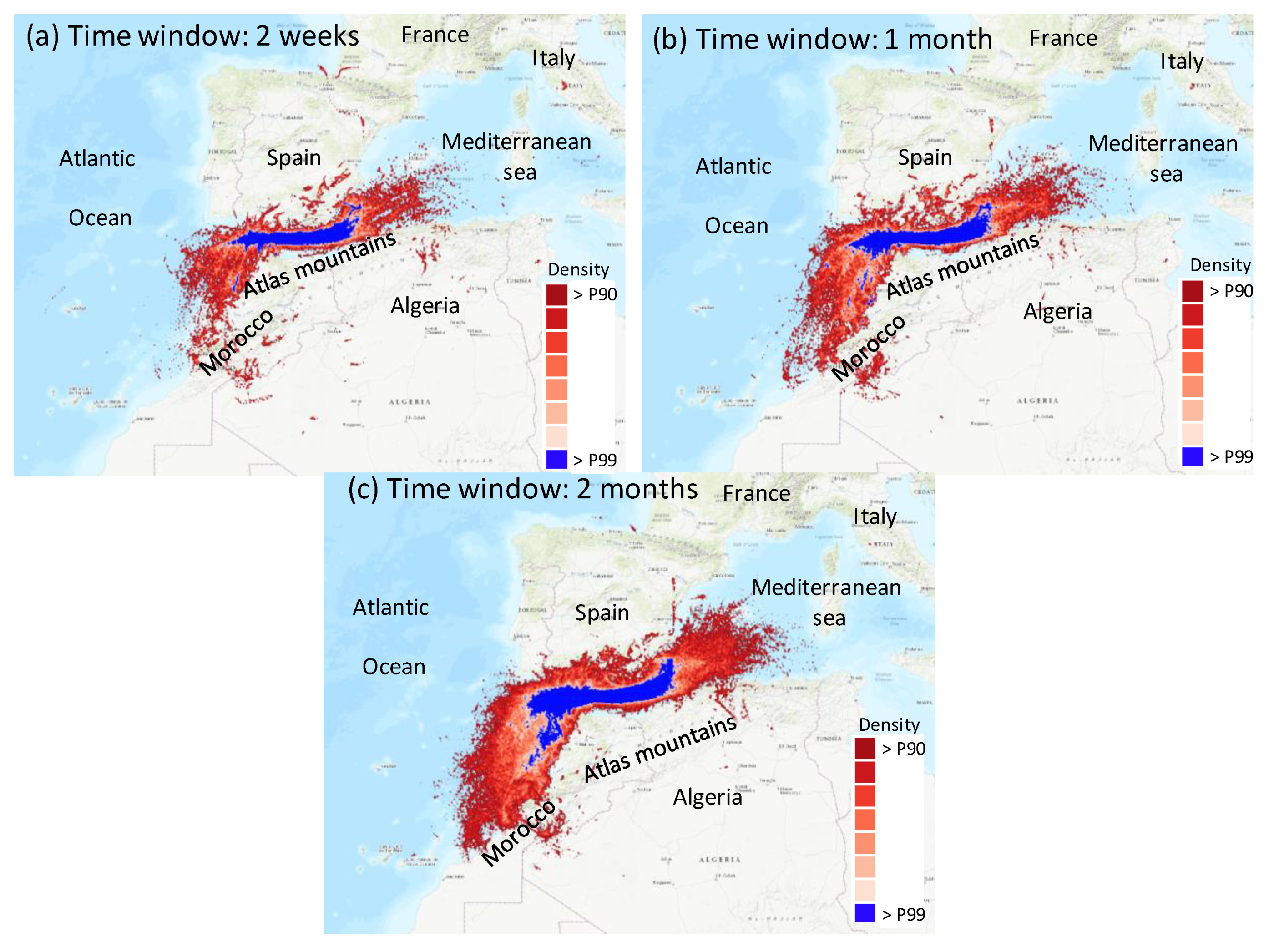
Table 1 shows the three time windows defined for each case study, taking as reference the corresponding release date to calculate the associated density map.
4. Results and Discussion
This section presents the set of density maps calculated for each case study. To evaluate the bias of our meteorological approach, the results obtained in the density maps are qualitatively compared with bibliography regarding the depositional analysis of each case study. We need to point out that our method does not aim to estimate the deposit, but the areas affected.
4.1. Chernobyl Accident
Figure 3 shows the density maps produced applying each one of the three time windows (
Table 1) for the period 2007–2016 from the Chernobyl site. The three maps display a large spatial dispersion from the release point. Our analysis finds high-density values (above the 90th percentile, P90) in central Europe and Scandinavia. This large dispersion provides an example of the differences in flow regimes, with areas being affected to the south (from southwest to southeast) and to the north of the release point. This spatial spread is in agreement with the variation in the meteorological conditions according to the release date. The emissions on 26 April were transported in the western and northern directions [
29], while the plume released in the following days started to move in a south-westerly direction, towards central Europe [
30], as well as towards Asia [
31].
The highest density values (above the 99th Percentile (P99); the blue circles in
Figure 3) in the three density maps are located to the southwest of the source region. This region covers areas of Romania and Bulgaria, such as the Western Romanian Carpathians, as well as the landmass formed inside the mountain circle, the Transylvanian Plateau and the Western Plain and Hills. The geographical distribution of elevated residence times in
Figure 3 is in agreement with most of the areas identified in the “Atlas of cesium deposition on Europe after the Chernobyl accident” [
32].
Figure 4 shows the high-resolution map of the total cumulative deposition of
137Cs throughout Europe as a result of the Chernobyl accident, which is used in this paper to validate the areas identified in
Figure 3.
Figure 4 shows that high deposits occurred in Eastern Europe and the Balkan countries, following the dominant precipitation. These areas are well identified in our density maps, which report the highest residence time values on the northern and southern borders of Romania.
Comparing the three maps (
Figure 3), the area with the highest density values is better identified on increasing the time window from two weeks to two months, i.e., the number of end-point positions, and hence, the meteorological scenarios. The impact of the time window on results is well observed by comparing the greater spread of spots with values above P90 between
Figure 3a (time window of two weeks) and
Figure 3c (time window of two months). This impact is especially seen to the south of the release site, as high-density values show up in the Black and Aegean seas, and northern Italy–southern Austria. In addition, zones in northern Germany and in the United Kingdom are identified by using a longer time window. In contrast, the set of areas identified in northern countries does not vary with the time window. In this region, few spots can be identified over continental areas, such as southern and eastern coastal areas of Sweden. In contrast,
Figure 4 displays a large spread of high
137Cs in specific areas of Sweden and Finland. One of the reasons of this difference can be associated with the selection of density values up to P90.
4.2. Algeciras Release
Figure 5 shows the corresponding density maps for the three time windows defined for the Algeciras case study. Density maps look similar for the three “time windows”, with the increase in the most affected area (>P90) easily seen by increasing the time window considered. The trajectories have either an eastern or southwestern component, displaying two main branches of the possible dispersion of the plume released at Algeciras. While the branch to the east, over the Alboran Sea, turns to the northeast following the Spanish coastline, the one to the west veers to the southwest following the northwestern coast of Africa. In both cases, after the channeling effect created by the southern Iberian Peninsula and northern African mountain chains, there is a wide area over the Atlantic and Mediterranean covered by high-density values.
The three maps display a wider area corresponding to the highest density values (above P99) to the east of the release site, along the southern Mediterranean coast of the Iberian Peninsula. It is interesting to highlight how this Mediterranean branch also presents areas over central Italy and northern Africa with high-density values.
This distribution is completely in agreement with the wind dynamics in this area, which is clearly conditioned by the channeling effect of the strait of Gibraltar [
33]. The highest density values are obtained to the east of the release site, over the Mediterranean Sea, being consistent with previous studies dealing with this event [
34], which reported an easterly movement of the plume. According to the measurements of
137Cs registered in southern France and northern Italy at the beginning of June, the radioactive plume continued its movement to the north-west over the Mediterranean Sea the following days. The density maps suggest this displacement, although the consideration of trajectories with a duration of 120 h limits the possible identification of continental areas affected.
5. Conclusions
This paper addresses the method developed to estimate the areas that could be most affected by harmful airborne releases to the atmosphere. To the author’s knowledge, this is the first study in which a long-term set of trajectories is used as part of an emergency preparedness infrastructure to early estimate areas likely to be affected by the release of harmful substances in the atmosphere. The bases for this approach are 5-days forward trajectories departing every 1 h at different heights above ground (in accordance with the study case) for the period 2007–2016.
We have qualitatively evaluated the method by comparing the results from density maps against the air concentration and deposition maps of 137Cs from the Chernobyl and Algeciras releases. The comparison reports a reasonable agreement in the identification of both the atmospheric dispersion patterns and the areas most affected by 137Cs activity concentrations.
Differences in the spatial coverage of the potential affected areas between these two events highlight the influence of the orography and of the release height in the transport and dispersion of substances in the atmosphere. While in Chernobyl (initial height of 1000 m a.g.l.), the transport occurs mainly above the boundary layer (1–2 km above surface) and hence, surface features affect the wind less (e.g., frictional drag); in Algeciras the wind is forced to move in a certain direction by the presence of mountains. In this sense, the Chernobyl map is a good example of the orographic blocking caused by the mountains, forcing the winds to slow down and/or change direction much more. The highest density values for the Chernobyl case study are found within the arc of the Carpathians and in the southern part of the country, in the Danube Plain, between the sub-Carpathians and Balkans. The main transport direction in the Algeciras case study is to the east, in agreement with previous studies.
The comparisons of density maps produced by different time windows (from weeks to months) have shown similarities in the identification of areas highly affected (>P99) by the air mass passage. The use of long time windows has produced the increase of the spatial coverage of these areas, but not the clear identification of new ones. The use of long time windows (more than one week before and after the release date), therefore, could not be necessary, as it could include the consideration of inhomogeneous and noisy trajectory endpoints.
While this method is far from being fully comprehensive, as only meteorological data are used, by building on the current results, future work with the purpose of including more years and measured concentrations into the analysis will help to further improve the present method, and to perform a quantitative evaluation.


