Article

Pre-Earthquake and Coseismic Ionosphere Disturbances of the Mw 6.6 Lushan Earthquake on 20 April 2013 Monitored by CMONOC

1
College of Geodesy and Geomatics, Shandong University of Science and Technology, Qingdao 266590, China
2
China Earthquake Network Center, Beijing 100045, China
*
Author to whom correspondence should be addressed.
Atmosphere 2019, 10(4), 216; https://doi.org/10.3390/atmos10040216
Submission received: 28 February 2019 / Revised: 8 April 2019 / Accepted: 20 April 2019 / Published: 22 April 2019
(This article belongs to the Special Issue Lithosphere–Atmosphere–Ionosphere Coupling (LAIC) Models)

Abstract

:
In order to study the coupling relationship between large earthquakes and the ionosphere, the techniques of ionosphere data acquisition were refined by the Crustal Movement Observation Network of China (CMONOC) to detect the pre-earthquake ionospheric abnormal and coseismic ionospheric disturbances (CID) of the Mw 6.6 Lushan earthquake on 20 April 2013. Based on the regional ionosphere maps (RIMs) derived from the Global Positioning System (GPS) observations of CMONOC, the ionospheric local effects near the epicenter of the Lushan earthquake one month prior to the shock were analyzed. The results show that the total electron content (TEC) anomalies appeared 12–14 (6–8 April), 19 (1 April), and 25–27 (24–26 March) days prior to the Lushan earthquake, which are defined as periods 1, 2, and 3, respectively. Multi-indices including the ring current index (Dst), geomagnetic planetary (Kp) index, wind plasma speed (Vsw) index, F10.7, and solar flares were utilized to represent the solar–terrestrial environment in different scales and eliminate the effects of solar and geomagnetic activities on the ionosphere. After the interference of solar–terrestrial activity and the diurnal variation in the lower thermosphere were excluded, the TEC variations with obvious equatorial ionospheric anomaly (EIA) in period-1 were considered to be related to the Lushan earthquake. We further retrieved precise slant TECs (STECs) near the epicenter to study the coseismic ionospheric disturbance (CID). The results show that there was clear STEC disturbance occurring within half an hour after the Lushan earthquake, and the CID propagation distance was less than the impact radius of the Lushan earthquake (689 km). The shell models with different altitudes were adopted to analyze the propagation speed of the CID. It is found that at the F2-layer with the altitude of 277 km, which had a CID horizontal propagation velocity of 0.84 ± 0.03 km/s, was in accordance with the acoustic wave propagation velocity. The calculated velocity acoustic wave from the epicenter to the ionospheric pierce points of this shell model was about 0.53 ± 0.03 km/s, which was also consistent with its actual velocity within the altitude of 0–277 km. Affected by the geomagnetic field, the CID mainly propagated along the southeast direction at the azimuth of 190°, which was almost parallel to the local magnetic line.

Graphical Abstract

1. Introduction

In the process of earthquake preparation and generation, a large mass of energy is released from crust. Except for destroying the earth’s surface, the energy even penetrates into the upper atmosphere, especially the ionosphere, and arouses corresponding abnormities [1]. To this day, the seismo-ionospheric anomalies have attracted extensive research attention in geoscience. On the one hand, there will be a considerable probability of ionospheric anomalies before shallow earthquakes, and ordinarily, a specific spatial–temporal feature of these anomalies is observed [2,3,4,5]. On the other hand, the coseismic ionospheric disturbance (CID) could be monitored by dense Global Positioning System (GPS) network sites near the epicenter. The research on the regularity of the propagation speed, waveform, and directivity of the CID is very important [6,7,8]. The analysis of pre-earthquake and coseismic ionospheric perturbations is no doubt of great significance in the deep exploration of the dynamic coupling mechanism of the lithosphere–atmosphere–ionosphere [9,10].
Since Forbes and Leonard [11] captured the seismo-ionospheric signals of the Alaska earthquake in the United States, the coupling relationship between the ionosphere and large earthquakes has gradually been mentioned and emphasized. Generally, apparent ionosphere anomalies are observed within several days or even hours preceding earthquakes. A statistical analysis, for example, of 14 large earthquakes (1966–2008) showed that 85.7% of cases had pre-earthquake ionospheric anomalies [12]. At present, the prevailing viewpoint on the coupling mechanism of pre-earthquake ionospheric anomalies is that the electromagnetic emission produced by the compression of underground rocks transmits to the surface, leading to the variations in particle concentration and the appearance of plasma irregularities [13]. The seismo-ionospheric anomalies usually have particular characteristics of the spatio-temporal distribution. Pulinets [14,15] found that the anomalous humps of the total electron content (TEC) usually drift toward the magnetic equator with the anomalous peaks shifting a certain distance from the epicenter. In addition, the magnitude of TEC anomalies is directly proportional to the magnitude and the time before the earthquake [3]. In earthquake generation, the atmospheric gravity wave (AGW) excited by tectonic activity is also a pivotal factor in causing coseismic ionosphere disturbances, which can be observed by the GPS network near the epicenter [16]. Comparing with ionosphere anomalies occurring before the earthquake, the amplitude of the CID was smaller (generally within 2 TECU, total electron content unit, 1 TECU = 1016 el/m2) and usually reached the utmost value within 10–20 min after the great shock, with a duration of only several minutes [8]. According to the CID propagation velocity, the excitation condition of ionosphere anomalies could be uncovered. Astafyeva et al. [7] measured two velocity components of CID generated by the Kurile seismic event (2009, Mw 8.1). The fast perturbation increased with distance the source (from 1.5 km/s (<800 km) to 2.5 km/s (>1800 km)), and the slow perturbation was approximately 0.7 km/s, which agreed with the results of numerical simulation for the Rayleigh surface wave velocity and acoustic velocity, respectively. The directivity in CID propagation is regarded as another research hotspot. For example, the investigation of Nepal earthquake (Mw 7.8, 2015) demonstrated that the influence of the geomagnetic field and rupture zone made it easier for the CID to propagate to the southeast of the epicenter [17].
Indeed, there are some disputes about the ionosphere responds to the Lushan earthquake on 20 April 2013. For example, Ma et al. [18] detected negative ionospheric anomalies near the epicenter from 18 to 20 April 2013, and considered them to be possibly related to the Lushan earthquakes. He et al. [19] observed the ionospheric disturbance on 4 March 2013, but attributed it to geomagnetic storm effects. Although they adapted rather different methods to construct the background field of ionosphere, both of them neglected the impact of the ionospheric short period of 27 days. This may result in diverse or even conflicting results.
In the paper, we made an attempt to study the effects of short-period variations in detecting the ionospheric anomalies before and after the Lushan earthquake. We adopted the geomagnetic planetary (Kp) and ring current index (Dst) to reflect the mid–low latitudes and global geomagnetic activities. The multi-index of solar activity was also used to discover the potential periods of solar abnormal activities from the outer atmosphere to surface regions of the sun. After analysis of the impact of the thermospheric variation and the correlation of regional TEC perturbation and solar–terrestrial factors, the seismo-ionospheric effects in different periods were evaluated. Then, a new method was further proposed to process the slant TEC (STEC) over the seismogenic area, and the coseismic ionospheric disturbances following the shock were investigated.

2. Data

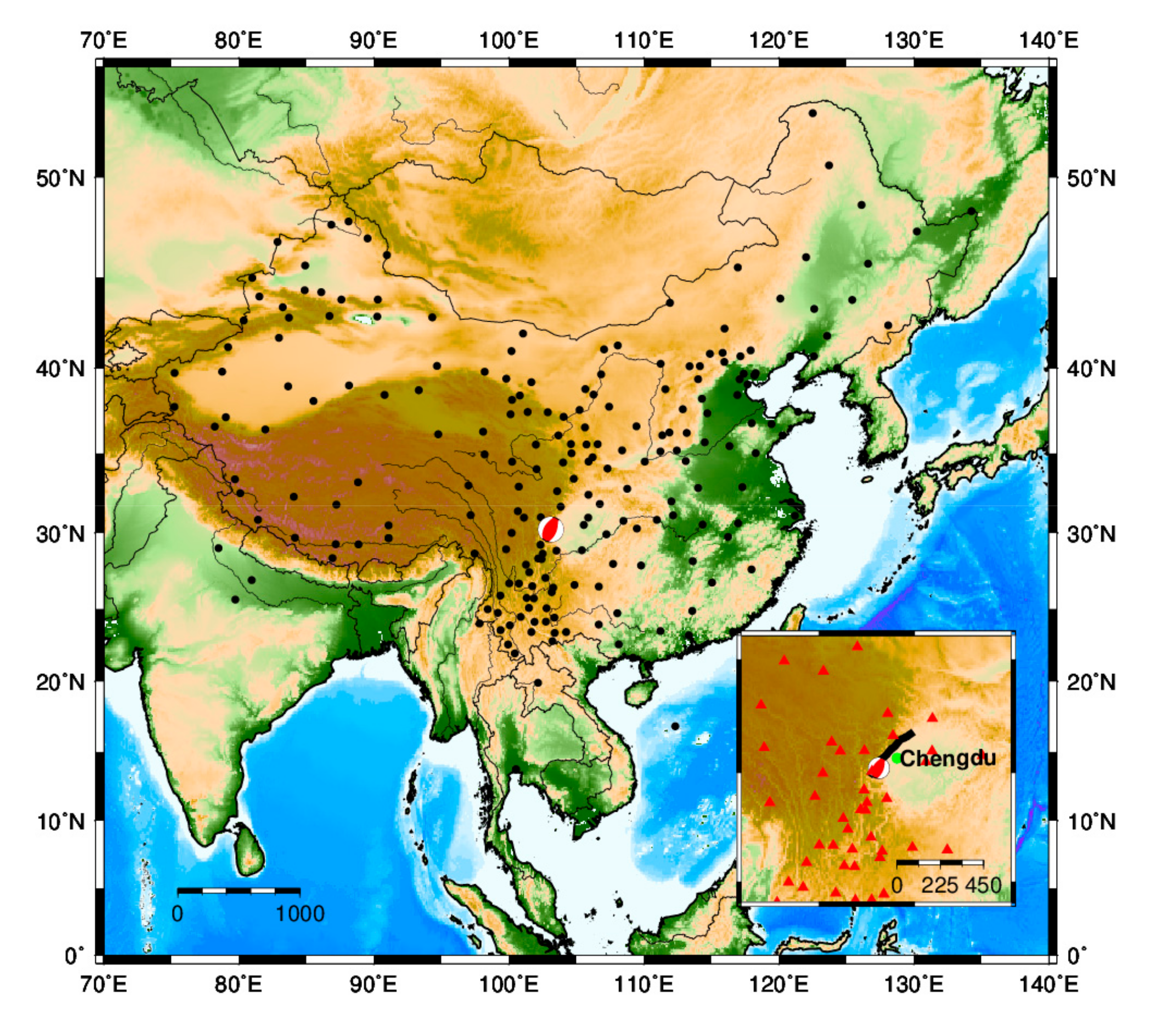
2.1. Space Environment Data

Due to the susceptibility of the ionosphere in relation to the external environment, the subtle ionosphere anomalies before the earthquake within a short period of time should not just consider the geomagnetic activities, but also attach the solar activities. Here, the Dst and Kp index provided by the Goddard Space Flight Center (GSFC) (https://www.nasa.gov/goddard) were used to represent the global and mid-latitude geomagnetic activities (ftp://ftp.ngdc.noaa.gov/STP/GEOMAGNETIC_DATA/INDICES). With a high correlation of the global TEC, the Kp index records the intensity of global geomagnetic field every three hours [10], and the Dst index can be used to estimate the effects of plasma drift on the ionosphere by magnetic storm in the mid–low latitudes. So, it is well suitable to describe the geomagnetic activities in different scales. Under the condition of geomagnetic calm, the Dst and Kp indexes are within ±30 nT and less than four, respectively.
The F10.7 index, solar flare (X-ray flux), and wind plasma speed (Vsw) observed by the GOES-15 satellite (http://www.sepc.ac.cn) were used to indicate the solar activity. The solar wind from the upper coronal layer is regarded as directly impacting the ionization of particles, leading to the distribution of the ion+ concentration. The solar wind speed was within 300–500 km/s, with an average speed of 350 km/s. The solar flare is one of the most violent explosive phenomena occurring in the local area of the solar atmosphere, and the M+ level flares are always accompanied by a sudden enhancement of particle radiation, releasing massive energy within a short period of time. The F10.7 with the unit of SFU (Space Environment Data, 1 SFU = 1022 W·m–2·Hz−1) is the index reflecting the variations of Extreme ultraviolet lithography (EUV) radiation in solar surface, which is the main ion+ resource of ionosphere. The F10.7 indexes of >150 SFU, 150–100 SFU, and <100 SFU reflect the solar activity from violence to weakness, respectively.

2.2. Ionosphere Data

The Coordinated Universal Time (UTC) here is adopted. On 20 April 2013, at 00:02:46 UTC, an Mw 6.6 earthquake hit Lushan County, Sichuan Province, China with depth of 14 km, and its epicenter was located at 30.28° N, 102.95° E, which was just about 100 km from Chengdu. Similar to the Wenchuan earthquake, the Lushan earthquake equally occurred in the Longmen fault belt, which is a vast NE–SW fault zone including three giant faults [20]. The previous studies have revealed that there was a vacant rupture zone with a length of nearly 50 km between the rupture surface of the Wenchuan earthquake and the Lushan earthquake, indicating a high seismic risk [21]. The CMONOC GPS station’s distribution over China is shown in Figure 1. Many of them are scattered over the mid-latitude region of China, with numerous sites covering the Longmen fault belt and adjacent areas. Using the CMONOC GPS data (http://www.neiscn.org/), we can derive the STECs and regional ionosphere maps (RIMs) for analyzing the pre-earthquake and coseismic ionospheric disturbance, extract the potential seismo-ionospheric signals, and ultimately, strengthen the real-time monitoring of the dangerous blank area.
By the dual-frequency GPS observations, the pseudo-range STECsll and STECslp are calculated from pseudo-range and carrier phase measurements, respectively:
S T E C s l l = 1 40.3   f 1 2 f 2 2 f 1 2 f 2 2 L 1 L 2 + λ 1 N 1 + b 1 λ 2 N 2 + b 2 + ε
And:
S T E C s l p = 1 40.3 f 1 f 2 2 f 1 2 f 2 2 P 2 P 1
where f, L, and P represent the carrier frequency, phase and pseudo-range observations respectively, the N1 and N2 are the ambiguities, and λ and b is the signal wavelength, and the hardware biases for carrier phase, respectively. Then, a baseline variable of Brs [22] was introduced as:
B r s = i = 1 T S T E C s l p i S T E C s l l i s i n 2 α i i = 1 N s i n 2 α i
among which T represents the effective sampling times when a satellite skims the top, and α was the satellite elevation angle. The high-precise STEC can be smoothed:
S T E C = S T E C s l l + B r s
To reduce the effects of large ionospheric horizontal gradients, GPS signals at elevation angles less than 15° are not considered. Due to the measurement error of the STEC with a 30-s time resolution reaching 0.01 TECU (total electron content unit, 1 TECU = 1016 el/m2) [23], the tiny ionosphere disturbance following the Lushan earthquake is easily observed. In this study, the single-layer shell model (abbreviated as the shell model) is adapted to analyze the seismo-ionospheric anomalies. When the ionosphere was assumed to be at a different altitude, the three-dimensional coordinate of ionospheric-pierce points was computed, and all the CIDs can be compared.
With a given ionospheric altitude of 450 km, the slant TEC is converted into the vertical TEC at the ionospheric pierce points using the mapping function:
V T E C = S T E C   c o s z
where z is the zenith distance of the signal path with respect to the vertical in a mean altitude of the single-layer ionospheric shell. Considering the inversion accuracy and efficiency, one regional single-layer ionospheric grid model over China is fitted with five-degree spherical harmonic function [24,25] to detect the pre-earthquake ionosphere anomalies. The RIM model over China from the GPS data of the Crustal Movement Observation Network of China (CMONOC) in 2013 is constructed with the geographical span of 15°–55° N and 70°–140° E, the spatial resolution of 1° × 1°, and the temporal resolution of two hours per day.
The global ionosphere maps (GIMs) that are provided by the international global navigation satellite systems service (IGS) are also used (ftp://cddis.gsfc.nasa.gov/gnss/products/ionex/) in the study. GPS data from global IGS tracking stations are processed to estimate TECs, which are used to construct GIMs with the time resolution of 2 h and the spatial resolution of 5° (longitude) × 2.5° (latitude). GIMs cover ±180° longitude and ±87.5° latitude. The GIM data are conducive to detect the equatorial ionospheric anomaly (EIA), which is an important signature of TEC disturbances in conjugate region.

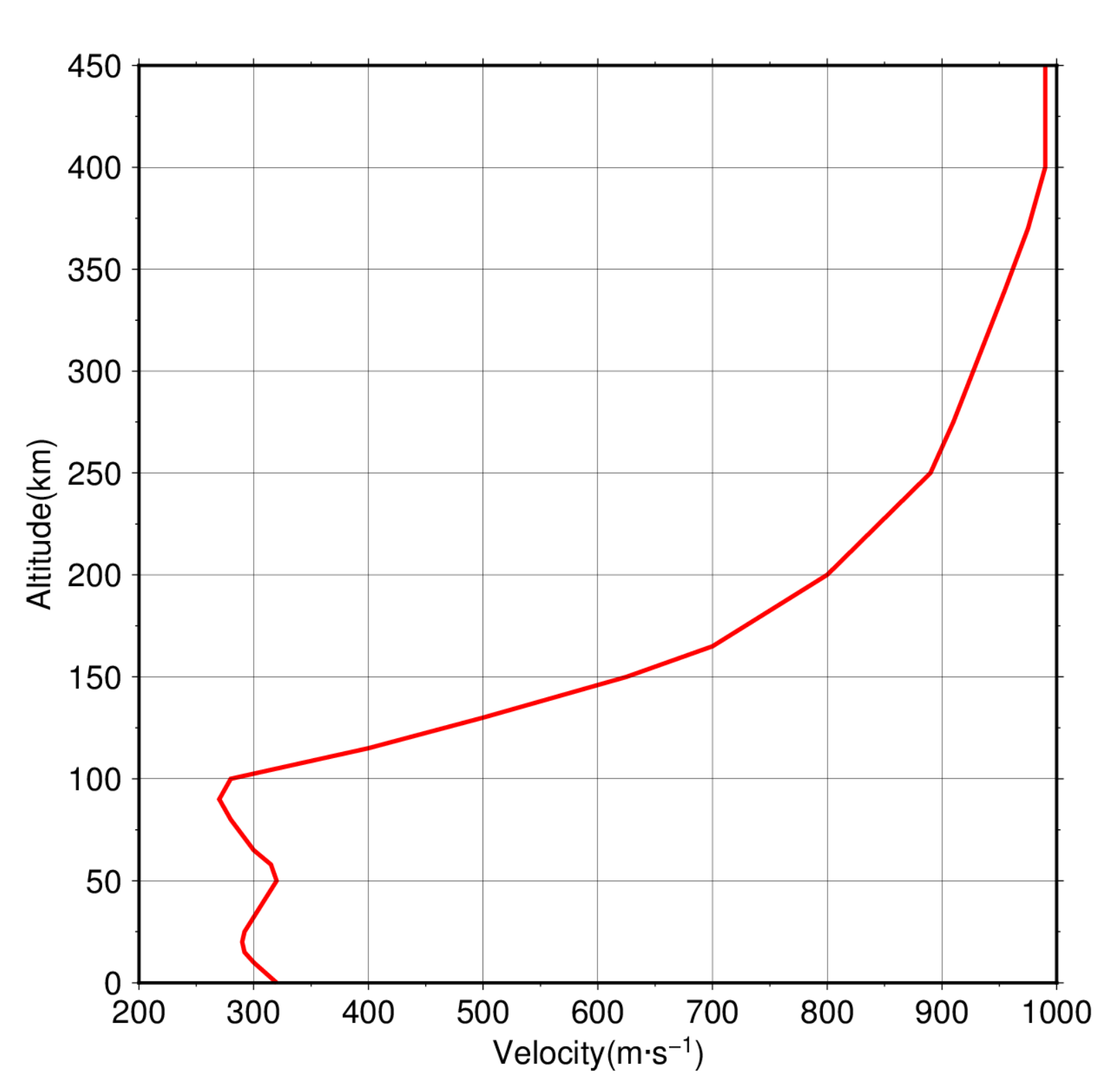
2.3. Electron Density Profile

The ionosonde observations of Zuoling station (ZLT) are utilized to achieve the electron density profile (http://data.meridianproject.ac.cn/). The vertical structure of the ionosphere in mid–low latitudes of China is less affected by longitude changes [26], and the latitude of ZLT (31.0° N) is close to the epicenter (30.3° N). It is well suitable to estimate the F2 layer altitude of the peak electron density over the epicenter according to the ZLT ionosonde observations.

3. Methodology

3.1. Interquartile Range Method

A 27-day periodicity caused by the solar rotation is the most prominent variation in short-term variations. Due to the influence of the solar activity, such as the ultraviolet ray and X-ray on the atmosphere, the ionosphere has a close correlation with the solar activity. The ionosphere has the same cycle as the solar activity of 27 days. Hence, in the verification of precursor signals, there might be certain difficulties if the time scale of 27 days is comparable to the leading time of several days of earthquakes [27]. More attention should be paid to the 27-day variation of solar radiation. In this paper, the sliding interquartile method is used to determine the pre-earthquake TEC anomaly. The interquartile range is a quantity in robust statistics to represent the discrete degree of data, and it is commonly used to check the data abnormality [28]. Here, the sliding averaged TEC of 27 days before required data is selected as the background value to weaken or eliminate the influence of periodic ionospheric variations. At the same time each day, the TECs are extracted and arranged into a sequence according to the ascending order: that is, x1, x2, x3…, x27. Then, the mid-quartile Q2 and interquartile range (IQR) can be obtained to take the Q 2 ± 2   I Q R as a threshold (~2.7 standard deviations) for TEC anomaly detection.

3.2. Singular Spectrum Analysis Method

In order to detect the weak seismo-ionospheric signals from the STEC, we need to remove its ionospheric background trend caused by the orbital motion of GPS satellites and temporal–spatial ionospheric variation [23]. The singular spectrum analysis (SSA) assists with extracting such principal component information from the ionosphere background containing the noises, and is mainly applied in studying the periodic oscillation of time series. Although it has been applied to many fields [29], the SSA is rarely used to detect the coseismic ionospheric disturbances. In this study, this method is used to investigate potential ionosphere disturbances following the Lushan earthquake.
The SSA consists of embedding a time series, singular value decomposition, grouping, and reconstruction. The STECs time series {x} ( x 1 , x 2 , …, x N ) is established during the shock eruption at 00:00–01:00 UTC, 20 April 2013 when the shock occurred, i.e. in the sight line of GPS PRN09-SCYY. Here, we define the length of {x}, N, as 120 according to the sampling of 30 s. The trajectory matrix X is constructed by selecting the appropriate window size M (<N/2) for the one-dimensional time series. The trajectory matrix X is calculated as:
X = x 1 x 2 x N M + 1 x 2 x 3 x N M + 2 x M x M + 1 x N
Giving the singular value decomposition to X , the reconstructed components (RCs) can be obtained and sorted according to the size of λ k   ( λ 1 λ 2 λ M 0 ). Generally, the greater the λ k , the richer the information the RCk contains. In the practical analysis, the low-order modes are selected. Therefore, the first few RCs are intercepted by the separation degree between different signals measured by w-correlation [30]. Eventually, the STEC disturbance signals (ΔSTEC) could be computed as:
Δ S T E C = S T E C S T E C m a i n
where STECmain as the principal component contains the ionospheric short-period signals and is obtained from the sum of selected RCs.

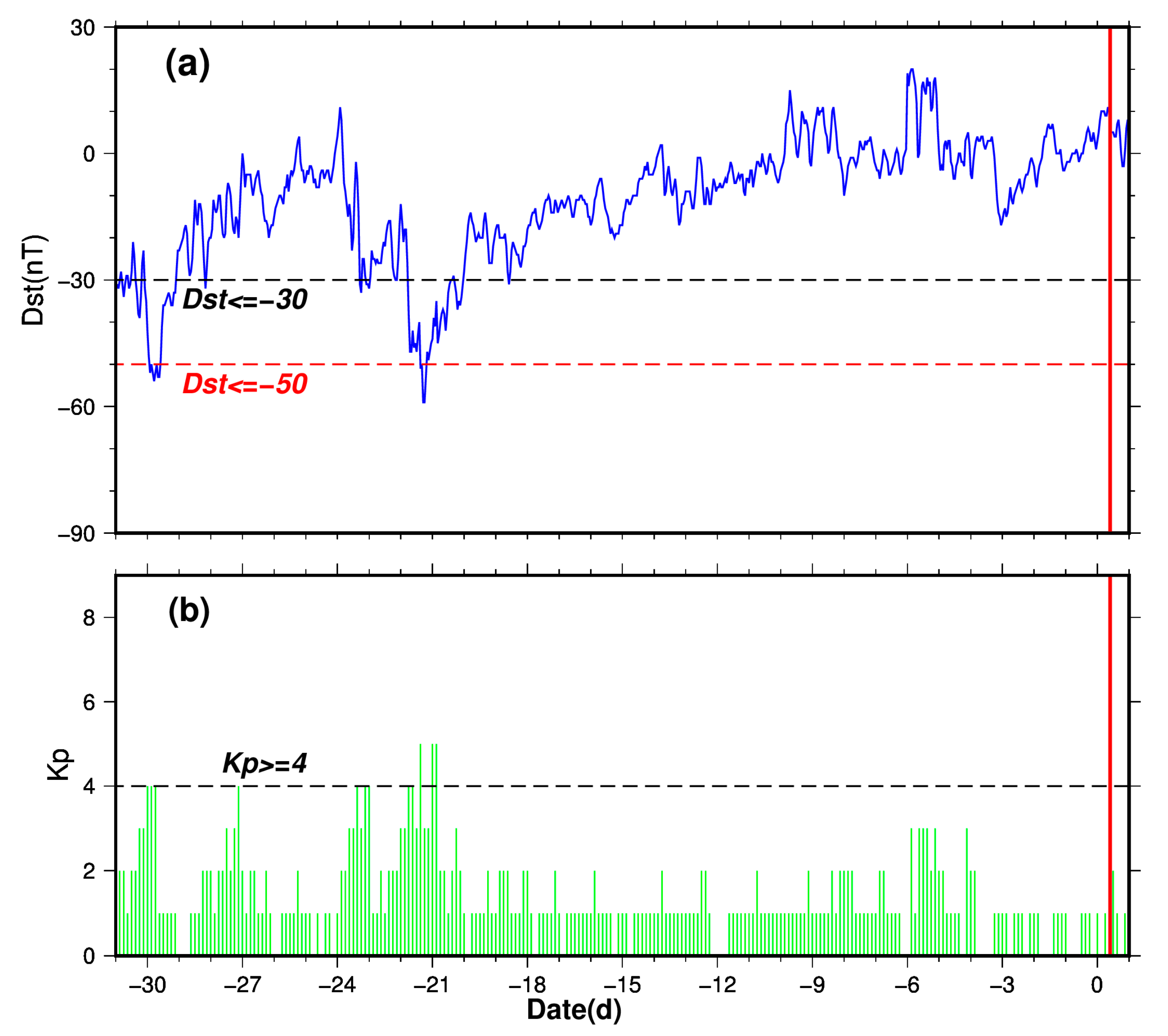
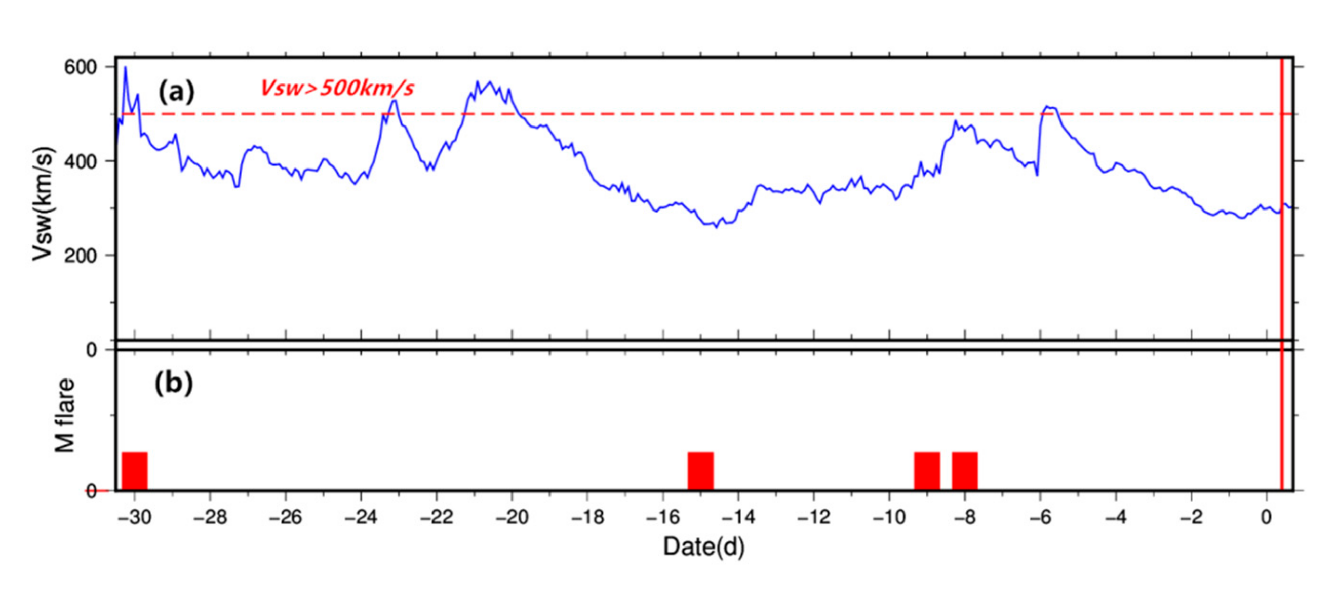
4. Solar–Terrestrial Environment

Before extracting the seismo-ionospheric signals of the Lushan earthquake, the effects of the solar–terrestrial environment as a major influence factor on the ionosphere should be excluded. The Kp and Dst index variations one month prior to the earthquake are given to judge the geomagnetic activity, as shown in Figure 2. Obvious geomagnetic disturbances were observed over two periods. The global medium magnetic storms of ~100 hours took place on 21 to 24 days prior to the earthquake (27–30 March), with the Kp reaching 5 and the Dst below −30 nT. The geomagnetic activity also had the small disturbance in the mid–low latitudes on the 30th day before the earthquake (21 March), with the Dst reaching 50 nT.
At mid–low latitudes, the level of solar radiation is dominant in determining the electron density of the ionosphere. The indices of radio flux F10.7 representing the levels of solar radiation have the same period of 27 days. Although the Lushan earthquake occurred during the period of high solar activity in the 24th solar cycle, there was no sudden change in solar activity (as shown in Figure 3), except for the 23 to 25 days prior to the shock (26–28 March) when the ΔF10.7 reached −8.5 SFU. Next, we continue to observe the variation of the index in X-ray flux and solar wind in Figure 4. It can be seen that the M flares occurred 30, 15, nine, and eight days before the Lushan earthquake (21 March, 5, 11, and 12 April), as well as on 26 and 28 March, when the Vsw reached beyond 500 km/s. The solar activity had a large fluctuation on the ionosphere in these periods, and remained stable for the rest of the time.

5. Ionospheric Anomalies Preceding the Lushan Earthquake

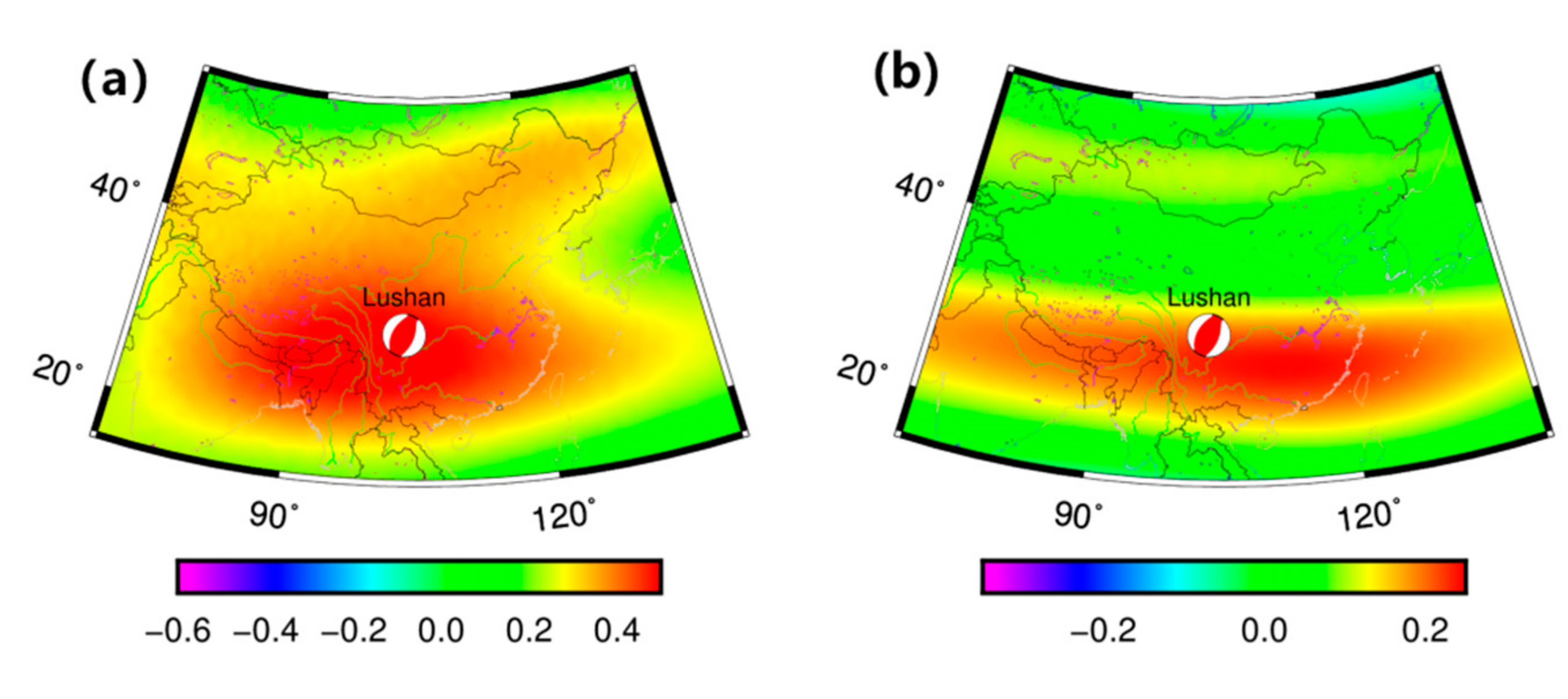
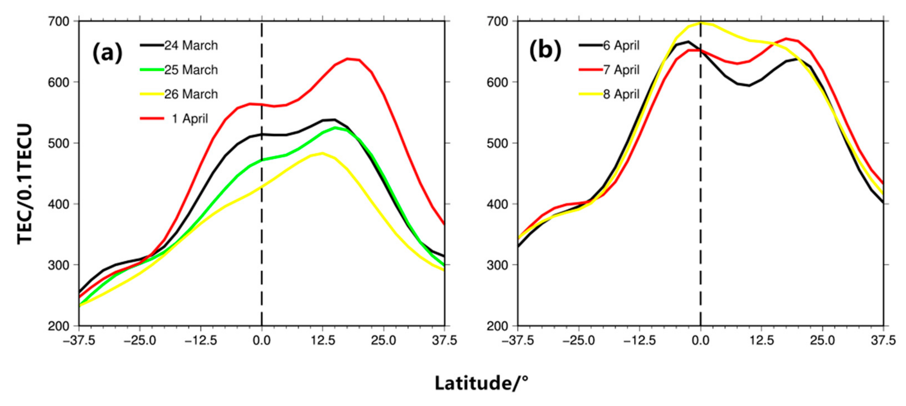
5.1. Distributions of TEC Anomalies

In order to examine the ionosphere variation of the epicenter, the TEC data of the closest grid of RIM (30° N, 103° E) to the epicenter (30.3° N, 103.0° E) were extracted. For most of the time, the TECs were within the upper and lower bounds. The TEC anomalies over the grid were analyzed with the interquartile range method, as shown in Figure 5. The main TEC anomalies appeared 12 to 14 (6–8 April), 19 (1 April), and 25 to 27 (24–26 March) days before the earthquake, with the maximum amplitude of more than 10 TECU, and these three periods were defined as period-1, period-2, period-3, respectively. In Figure 2, Figure 3 and Figure 4, the pre-earthquake solar and geomagnetic activity was abnormal in period-3. So, whether the TEC anomalies in the period were caused by the external environment needs to be further analyzed.
During period-1 and period-2, most of the violent TEC turbulence appeared on 1 and 6 April respectively, which was regarded as the representative dates of both periods. Therefore, the 27-days TEC data before 1 and 6 April were extracted, and the detailed analysis of the TEC anomaly over China on both days was processed by the interquartile range method, as shown in Figure 6. The detection based on RIMs showed a major distribution of ionosphere anomaly to the south of the epicenter. A sizeable east–west span of the ionosphere abnormality, reaching 70° occurred on 1 April, while on 6 April, the length–width ratio of the abnormal region was close to 3:1, which coincided with the previous studies of ionosphere anomaly before Mw 9.0 Tohoku (11 March 2011) and Mw 7.8 Wenchuan earthquakes (12 May 2008) [31,32]. Differing from a rather close distance between TEC anomalous peaks and the epicenter in period-1, the epicenter in period-2 was located at the edge of abnormal regions with a large displacement.
To analyze the dynamics of the EIA for the Lushan earhquake, a strip along the 105°E meridian at a local time (LT) of 11:00 (4:00 UT) was selected (see Figure 7) from the GIM source. Although the magnetic storm happened in period-3, the shape of the EIA was relatively stable. It seemed that the EIA does not seem to be affected by the geomagnetic conditions. On 1 March in period-2, the EIA enhancement, by contrast, may be attributed to the positive TEC anomalies. Especially, the change of its northern crest can be validated in Figure 5 and Figure 6. From Figure 7b, a signal with the appearance of a double-peak structure in EIA was readily captured. While the TEC value at 105° E meridian kept on rising, and its double-peak structure subsided gradually from 6 to 8 April, implying the ionosphere disturbances with a conjugated structure in period-1.
Currently, ionospheric variability can be attributed to three potential sources, that is, (1) changes of the solar ionizing flux, (2) geomagnetic storms, and (3) “other” or “meteorological” influences [33]. The disturbances of solar–geomagnetic activities can either cause widespread electron density enhancements or depletions. The ionospheric variability of the third “meteorological source”, on the contrary, is thought to present certain spatial–temporal regularity [4,5]. While ionospheric precursor studies have typically eliminated solar and geomagnetic activities as the causes of a particular anomaly, the thermospheric contributions are usually overlooked or underestimated [34]. From Figure 5, it can be seen that specific distributions of TEC anomaly emerged during period-1 and period-2 when the solar–geomagnetic activities were stable. With significant local effect in the epicenter, the TEC anomaly shifted toward the magnetic equator, and even ionosphere disturbance with a full conjugated structure was found in period-1. However, we are still not sure whether both anomalies were related to the Lushan earthquake, because such ionospheric variations might be caused by possibly day-to-day disturbances in the lower thermosphere.
In the next section, an investigation of authentic accounts to the TEC variations will be conducted based on the RIM model. In addition, the impact of the external environment will be further evaluated in two ways. Firstly, the TECs over the epicenter during one year before the Lushan earthquake were extracted to analyze the responses of the ionosphere to the magnetic storm. Then, the cross-wavelet analysis will be introduced to analyze the correlation between ionospheric anomalies and the solar–terrestrial environment.

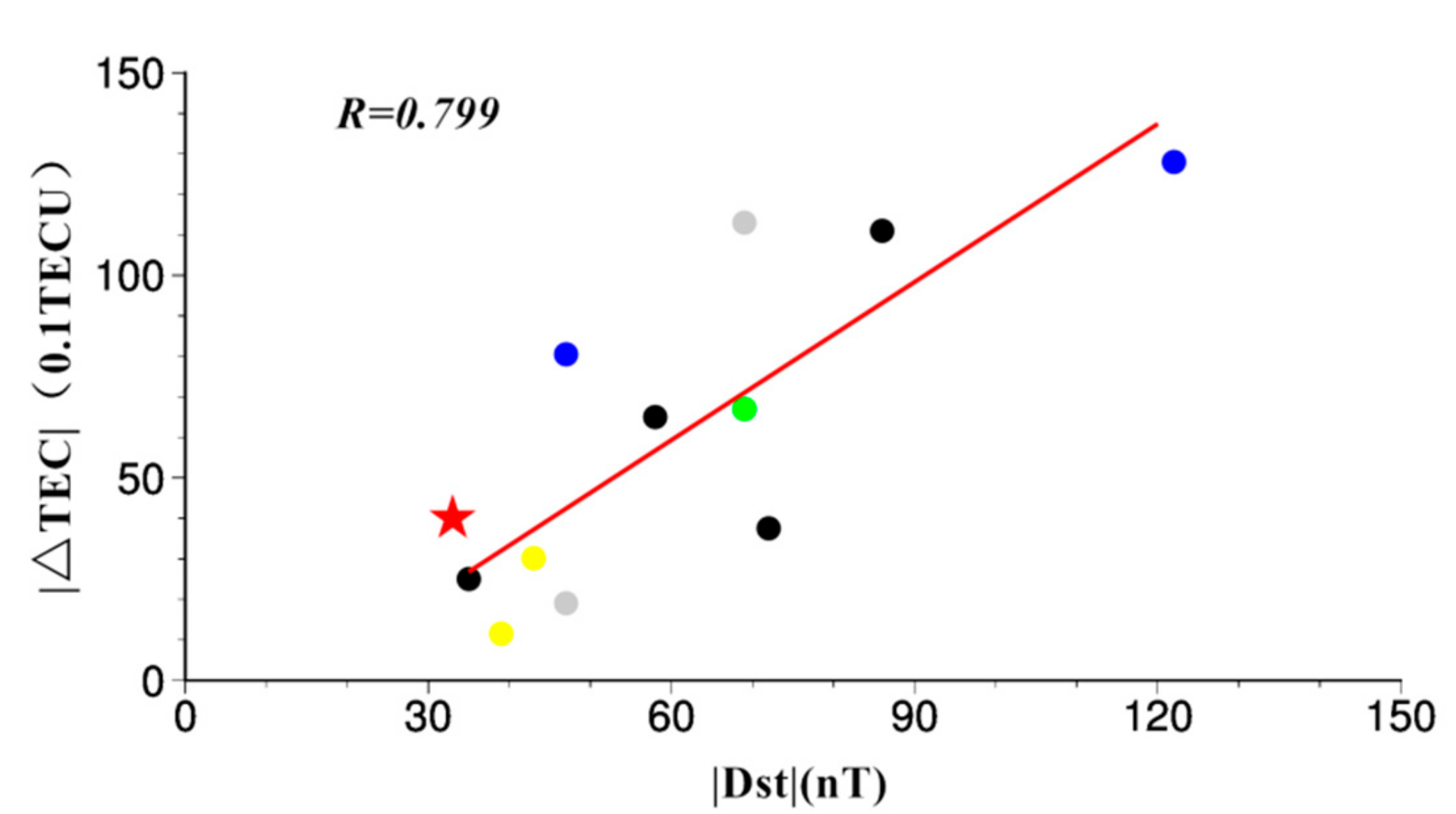
5.2. The Effects of the Variations in Space Environment and Thermosphere Structure

We used one-year TECs over the epicenter to study the ionospheric anomalies, and the results are shown in Figure 8. Here, the level of geomagnetic activity (Dst) at the time of detection is also displayed. There were 10 extra occurrences of anomalies in the one-year period, including the dates of 16–19 June, 15 July, 2–3 September, 1–2 October, and 29–30 November 2012. Almost all the days were accompanied by magnetic storms, and a certain proportional relation between |Dst| and |ΔTEC| value can be seen. Therefore, the likelihood that these anomalies were unique to seismic activity was low. The finding was in accord with that of [19].
The diurnal variation in the thermosphere is usually not taken into account, which is an essential reason for the inconsistent statistical results of pre-earthquake ionospheric anomalies [34]. Normally, such relative TEC variability (to the last day) did not exceed 30% [35]. We calculated the value of TEC diurnal on both days to exclude the meteorological effects, as shown in Figure 9. As seen from Figure 9, the anomaly amplitude on 6 April 2013 far exceeded the limit of 30%, indicating that the ionospheric disturbances were independent of thermospheric variations. Due to the maximum amplitudes of around 30% on 1 April, however, it is difficult to determine whether the TEC anomalies in period-2 were related to the earthquake.
In the study, the correlation between ionospheric anomalies and solar environment were verified by the cross-wavelet analysis [36]. Usually, with the relative phase relationship as arrows, the 95% significant level against red noise is shown as a thick contour. If the power is enclosed by the thick contour, it would pass the significance test. The brighter or more intense the color presents, the higher the correlation of both time series.
The correlation on ΔTEC and Vsw were given in Figure 10. With a light color, the power in period-1 did not pass the correlation significance test, showing a low correlation of both indices and a limited shock of solar wind (<300 km/s) to the ionosphere anomalies. In a word, under the stable conditions of the solar–geomagnetic activities in period-1, the TEC anomalous enhancement in period-1 was considered to be probably caused by the Lushan earthquake.

6. Analysis of Coseismic Ionospheric Disturbances

6.1. Disturbance Signals Extraction and Waveform

Before extracting the disturbance signals of the STEC, its principal component, STECmain needs to be removed chiefly. By w-correlation, the separation degree of the reconstructed components was judged to screen out the essential trend–periodic terms. These RCs with small w-correlation values were usually treated as noises [37].
The SCYY tracking station in Yanyuan county, Sichuan province could receive continuous GPS PRN09 signals from 00:00–01:00 UTC on 20 April 2013, with the lowest elevation angles at 70°, and was only 220.1 km to the epicenter. Therefore, the STECs of the SCYY station to GPS PRN09 following ~1 h after the shock was derived as a case to clarify the extraction of the disturbance signal. After the singular value decomposition of the STEC time series, the w-correlation values of the first 15 RCs were computed, as shown in Figure 11. It is clear that the first five RCs had better independence than the latter, and contained the primary information of original series with the cumulative contribution rate over 95%. By culling the first five RCs as STECmain values from the STECs, the disturbance signal of the ionosphere was obtained, as shown in Figure 12.
Within one hour, the STEC varied from 54 TECU to 62 TECU, and a tiny disturbance started from 00:14:00 UTC. In comparison, a more significant change occurred in the ΔSTEC series, with the first trough value of 0.05 TECU at 0:15:00 UTC, the peak value of 0.1 TECU at 0:16:00 UTC, and the last trough at 0:17:30 UTC. The ionosphere anomalies lasted nearly 4 min, and returned to normal after 0:18:00 UTC. This “N” typed waveform in STEC conformed to the characteristics of ionosphere disturbances induced by strike-slip earthquakes [38].
Except for the insurance of continuous signals from GPS satellites, it is vital that visible disturbance should appear in the STECs along the signal transmit path following the Lushan earthquake. Thus, the selection of proper GPS satellites was essential to improve the effectiveness of detecting the coseismic ionospheric disturbances. Also, the work was carried out based on the STEC derived from the received signals of SCYY stations, and the detective results of ionosphere disturbance from 00:00–01:00 UTC on 20 April are shown in Figure 13. It can be seen that significant disturbances were detected in the ΔSTEC time series of PRN09 and PRN16 from the SCYY station with a continuous “N” typed waveform. While the abnormal amplitude of both STEC curves was similar, reaching 0.10 TECU and 0.11 TECU, respectively, and their disturbance durations were all 3.5 min, the perturbed signals started at different times, about 11 min and 16 min after the shock, respectively. Apparently, CID propagation presented directional differences.
According to the relationship between impact range and the magnitude of the earthquake (denoted as M), the size of earthquake preparation zones (denoted as R) [39] could be determined as:
R = 100.43M
Associated with a magnitude of Mw 6.6, the radius of the affected area of the Lushan earthquake was 689 km. Next, the GPS data of the PRN09 and PRN16 satellites within the seismogenic area would be adopted to further analyze the CID propagation characteristics.

6.2. Disturbance Velocity and Altitude

In the paper, the study of CID was based on the single-shell layer model. In fact, the CID has a three-dimensional structure in the ionosphere of finite thickness. It is unavoidable that the feature analysis of CID propagation will be affected along with the alternation of the assumed thin-ionosphere altitude [40]. The electron density profile over the epicenter at 00:00 UTC following the Lushan earthquake was estimated by the ionosonde observations of the ZLT station (see Figure 14). Following Calais et al. [41], a simple ray tracing in the atmosphere was also performed with altitude-dependent acoustic velocity, as shown in Figure 15. Then, the shell-1 model at the altitude of 277 km with an actual maximum electron density and the shell-2 model at 450 km, which are frequently used in many studies, were respectively assumed to identify an appropriate model to explain the reason for the formed CID.
In analyzing the STEC disturbance, the coordinate of sub-ionospheric points (SIPs) was deduced from the location of ionospheric pierce points, namely the intersection point from the satellite-receiver line to thin layers. Then, the propagation velocity of disturbance could be calculated by the ratio of the distance of SIPs to the epicenter to the time delay of perturbation.
Figure 16 shows the relationship among the ΔSTEC, CID occurrence time, and the distance to the epicenter at 00:00–01:00 UTC on 20 April 2013. Some CID points were detected ~10 min after the earthquake, and the disturbance duration and maximum amplitude reached 10 min and 0.22 TECU, respectively. In addition, there was a slight difference in the abnormal range of both models, with epicentral distances of 68–642 km (shell-1 model) and 45–586 km (shell-2 model).
According to the occurrence time and epicentral distance of the CID peaks, the best connection line representing the horizontal propagation speed of CID was fitted with the least-squares fitting method. The CID propagation velocities of both shell models reached 0.84 ± 0.03 km/s (shell-1 model) and 0.76 ± 0.03 km/s (shell-2 model), while at the altitude of 277 km and 450 km, the propagation velocity of the acoustic wave was about 0.92 km/s and 0.98 km/s, respectively. The apparent coincidence justifies the assumed altitude of the shell-1 model, which nearly corresponds to the maximum electron density.
Figure 2 has revealed that the solar–terrestrial environment was quiet in the period with the Kp index of 1 and the Dst index of 5 nT. From the proportional amplitude–distance relation of CID and a fixed propagation speed, it can be inferred that the coseismic ionospheric disturbances were triggered by the seismic waves of the Lushan earthquake.
In support of the proposed shell-1 model, the velocity of the seismic wave during propagation from the epicenter to each ionospheric-pierce point was further estimated and compared with the actual velocity. A total of 14 tracking stations have captured the CID signals, and the SIP’s epicentral distance of CID peaks, the corresponding occurrence, and the estimated acoustic velocity were listed in Table 1. Table 2 lists the statistic results. At different thin-shell altitudes, the SIP’s epicentral distance and corresponding acoustic velocity varied greatly. From Table 2 and Table 3, it can be seen that while the shell-1 model was adopted, the velocities of the acoustic wave from the epicenter to the ionosphere altitude of 277 km were calculated, varying from 0.47 to 0.60 km/s, and the average and standard deviation value were 0.53 and 0.03 km/s, respectively. If we changed the ionospheric altitude to 450 km in accord with the shell-2 model, the estimated acoustic velocity ranged from 0.56 km/s to 0.72 km/s, with the average and standard deviation values of 0.65 km/s and 0.05 km/s, respectively. Obviously, among the 14 stations, the estimated velocities of the acoustic wave had a larger difference than those of the shell-1 model.
Figure 15 also showed that from the ground to the assumed ionosphere altitude of both models, the average velocity of the acoustic wave is ~0.54 km/s (0–277 km) and 0.71 km (0–450 km). Therefore, the estimated velocity based on the shell-1 model better matches the actual velocity than the shell-2 model, which further supports the setting rationality of ionospheric altitude at the maximum electron density.

6.3. Directivity of the Propagation

The location of the CID peaks was calculated based on the shell-1 model, and their amplitudes were also illustrated (seeing Figure 17). A negative correlation between the amplitude of the CID and the distance to epicenter was found, and the propagation range was limited within the impact radius of the Lushan earthquake. A universal opinion is that the topography and earthquake fracture zone impacted the propagation of the CID caused by the Rayleigh surface wave [17]. However, our study showed that the ionosphere anomaly following the Lushan earthquake was aroused by the propagation of acoustic waves released from the earthquake to the thin ionosphere. As shown in Figure 17, at the F2-layer altitude, a clear north–south asymmetry has been found, which could be attributed to the local geomagnetic field. In acoustic waves, an inverse movement trend of particles oscillates in the north–south hemisphere. Significant ionosphere disturbances to the north of the epicenter are easily recorded in the southern hemisphere, while CID in the southern hemisphere tend to propagate in the north [42]. In the equatorial region, the ionosphere disturbance propagated both in the north and south directions. Consistent with the rule, Figure 17 also showed that the CID mainly propagated to the south of the epicenter at the azimuth of 190°, and the amplitude of ionosphere disturbance along this direction far exceeded that in the northern part of the epicenter.
Following the model of International Geomagnetic Reference Field in 2012 (IGRF 12) (https://www.ngdc.noaa.gov/geomag-web/), the data of the total strength of the geomagnetic field and the magnetic inclination angle within the seismogenic area was simulated. As shown in Figure 17, the magnetic field strength near the epicenter was greatly influenced by latitude, while the magnetic inclination angle showed a small variation from 0.5° E to 3.7° E. The ionospheric coupling factor k [17] was introduced as:
k = cos β
where β is the angle between the neutral velocity and the geomagnetic field vector. The k value to the north of the epicenter (0.1–0.6) was lower than that to the south of the epicenter (>0.7). The SIPs with k values beyond 0.9 concentrate at the main transmission line, which was approximately parallel to the horizontal projection of the magnetic field line. Hence, the local magnetic field played a decisive role for the directivity in CID propagation.
Generally, the ionospheric disturbances during the coseismic process may be caused by three kinds of seismic waves: the acoustic–gravity waves generated by the vertical movement of the Earth’s surface, the gravity waves tilted upward from the focal area or the tsunami, and the infrasonic waves aroused by the Rayleigh waves [7]. However, CID amplitude usually increased with increasing Mw and a threshold magnitude of near Mw 6.5 [43]. The relatively small magnitude of the Lushan earthquake (Mw 6.6) led to only one kind of seismic wave being detected. With the help of the CMONOC, the follow-up work will continually monitor more earthquakes to develop the seismo-ionosphere coupling mechanism.

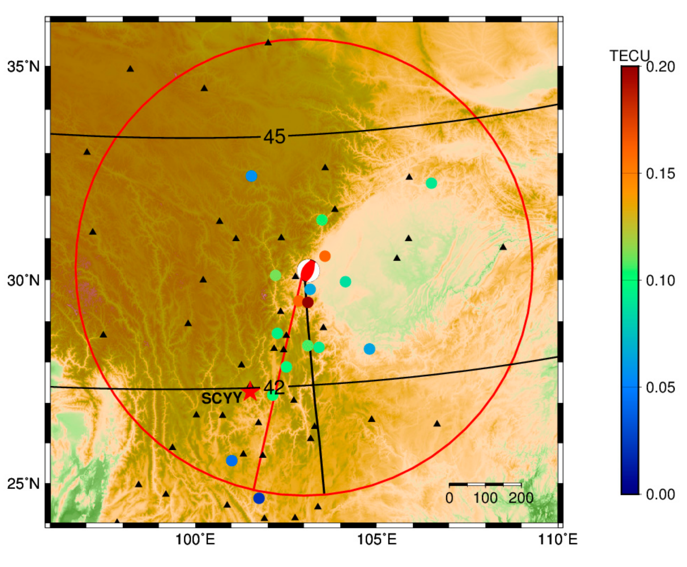
6.4. Determination of Epicentral Location

Generally, the vertical motion of the Earth’s surface in an earthquake arouses the acoustic waves, which propagate upward to the ionospheric height, interact with the plasma, and then spread around in a nearly horizontal direction. This leads to the generation of ionospheric disturbances. According to the theory, we adopt the ray-tracing model [44] to compute the coordinate of the CID source with a grid search method.
A specific hunting zone (25°–35° N, 80°–100° E) is initially chosen to find the optimal grid point by shifting the grid of 0.1° (longitude) × 0.1° (latitude). Based on the shell-1 model, the horizontal propagation velocity of CID, VH, has fitted above at 0.84 km/s. The occurrence of the CID source TAK is given as:
TAK = TCK − DHK/VH
where DHK is the horizontal distance from the CID peak to the CID source, and TCK is the observation time of the CID peak. There are N CID points used, whose TAK values and corresponding standard deviation (unit: s) can be obtained. By shifting these grids, the final CID source can be determined when the standard deviation of the hunting grid reaches a minimum, and the results of the optimal grid coordinates are shown in Table 3.
The final CID source was estimated at 30.9° N and 101.5° E, which is a slight deviation of 74.7 km to the southeast from the epicenter. Apart from the non-coincidence of the point of maximum energy release in the earthquake and the location of the epicenter, the ionospheric neutral wind would also affect the CID propagation.

7. Conclusions

Based on the TECs derived from CMONOC GPS data, an attempt was made to detect the pre-earthquake and coseismic ionospheric disturbances associated with the Mw 6.6 Lushan earthquake on 20 April 2013. By analyzing the ionospheric anomalies over the epicenter, it is found that the TEC anomalies occurred in three periods: that is, 24–26 March, 1 April, and 6–8 April 2013. On 6 April, the noticeable local signatures of TEC turbulence were observed. The TEC anomalies shifted toward the west along the equatorial anomaly boundary with peaks appearing near the epicenter. A more macro scale of ionosphere disturbances with a full conjugated structure on this day were also registered by analyzing the EIA phenomenon. After considering the variations proportion (to the previous day) exceeding 30% and the stable solar–terrestrial activity, we concluded a potential possibility of the TEC anomalies on 6–8 April caused by the Lushan earthquake.
By using the GPS data from continuous tracking stations near the epicenter, the STECs were computed to analyze the CID of the Lushan earthquake. The CID was registered with maximum amplitudes of 0.22 TECU, and a duration of 10 min. According to the ionosonde observations at ZLT station, the altitude of the single-layer shell was set at the F2-layer with the altitude of 277 km. At the altitude, it was found that the horizontal propagation speed of CID was consistent with the propagation velocity of the atmospheric acoustic wave. Based on the occurrence and coordinate of CID, we deduced the average velocity of the acoustic wave from the epicenter to the ionosphere. Similarly, the results revealed that the estimated velocity of the acoustic wave also coincided with its actual propagation velocity. In CID propagating, we further monitor that the coupling factor k in the main transmission line of CID reached 0.9, which was far beyond the north region of the epicenter. It implies that the local geomagnetic field was a critical reason affecting the propagation of ionosphere disturbance, and the complete presence of the southern disturbance to the epicenter might be explained by the high ionospheric coupling factor. Besides, the intensity and waveform of the CID was easily affected by the magnitude and type of earthquakes. The neutral wind also made the CID source that was determined slightly deviate from the epicenter.
The contribution of 27 days of solar radiation variation on ionospheric variation and the eruption of the solar activity such as the solar wind and sun flare should be taken into account in discriminating ionospheric anomalies related to earthquakes [45]. In fact, the influence of geomagnetic and solar activities on the ionosphere is very complex, and there is a wide difference in the ionosphere responses under different geomagnetic–solar environments. Other limits, such as the irregularities of the ionosphere and the defect of GIMs, make it rather difficult to determine the seismic–ionospheric signals. Besides, the investigation of coseismic ionospheric disturbance also depends largely on the dense GPS networks. Inevitably, these problems have hindered the further development of seismo-ionospheric anomaly detection. As a preliminary exploration in the study, more statistics of earthquake cases in the future will be investigated, so that the pure features as precursor signals could be extracted, and the corresponding coupling physical mechanism would be improved.

Author Contributions

K.S. was involved in STEC/TEC derivation, drawing images, and conducting the manuscript writing. X.L. and J.G. contributed to the study design and the analysis of seismic–ionospheric anomaly and discussion. L.L. focused on the collection and compilation of documents. F.W. and X.Y. helped collect the CMONOC GNSS observations. All the authors read and approved the final manuscript.

Funding

The Institute for GPS meteorology was supported by the National Natural Science Foundation of China (grant No. 41774001 & 41704015), the Shandong Natural Science Foundation of China (grant No. ZR2017MD032), the SDUST Research Fund (grant No. 2014TDJH101) and the Research and Innovation Team Support Program of Shandong University of Science and Technology (grant No. SDKDYC180207).

Acknowledgments

We are very grateful to the China Earthquake Network Center for providing CMONOC GPS data, the International GNSS Service for providing GIM data, and the Goddard Space Flight Center. The Space Environment Prediction Center is acknowledged for M flares data.

Conflicts of Interest

The authors declare that they have no competing interests.

References

  1. Sorokin, V.M.; Chmyrev, V.M.; Yaschenko, A.K. Theoretical model of DC electric field formation in the ionosphere stimulated by seismic activity. J. Atmos. Solar-Terr. Phys. 2005, 67, 1259–1268. [Google Scholar] [CrossRef]
  2. Liu, J.Y.; Chen, Y.I.; Pulinets, S.A.; Tsai, Y.B.; Chuo, Y.J. Seismo-ionospheric signatures prior to M ≥ 6.0 Taiwan earthquakes. Geophys. Res. Lett. 2000, 27, 3113–3116. [Google Scholar] [CrossRef]
  3. Le, H.; Liu, J.Y.; Liu, L. A statistical analysis of ionospheric anomalies before 736 M6.0+ earthquakes during 2002-2010. Geophys. Res. Lett. 2011, 116, A02303. [Google Scholar] [CrossRef]
  4. Guo, J.; Li, W.; Liu, X.; Wang, J.; Chang, X.; Zhao, C. On TEC anomalies as precursor before Mw8.6 Sumatra earthquake and Mw6.7 Mexico Earthquake on 11 April 2012. Geosci. J. 2015, 19, 721–730. [Google Scholar] [CrossRef]
  5. Guo, J.; Li, W.; Yu, H.; Liu, Z.; Zhao, C.; Kong, Q. Impending ionospheric anomaly preceding the Iquique Mw8.2 Earthquake in Chile on 1 April 2014. Geophys. J. Int. 2015, 203, 1461–1470. [Google Scholar] [CrossRef]
  6. Calais, E.; Minster, J.B.; Hofton, M.; Hedlin, M. Ionospheric signature of surface mine blasts from Global Positioning System measurements. Geophys. J. Int. 1998, 132, 191–202. [Google Scholar] [CrossRef]
  7. Astafyeva, E.; Heki, K.; Kiryushkin, V.; Afraimovich, E.; Shalimov, S. Two-mode long-distance propagation of coseismic ionospheric disturbances. J. Geophys. Res. 2009, 114, A10307. [Google Scholar] [CrossRef]
  8. Heki, K. Ionospheric electron enhancement preceding the 2011 Tohoku-Oki Earthquake. Geophys. Res. Lett. 2011, 38, 1585–1593. [Google Scholar] [CrossRef]
  9. Afraimovich, E.L.; Feng, D.; Kiryushkin, V.V.; Astafyeva, E.I. Near-field TEC response to the main shock of the 2008 Wenchuan earthquake. Earth Plants Space 2010, 62, 899–904. [Google Scholar] [CrossRef]
  10. Li, Z.; Tang, L.; Zhang, X.H. Ionospheric disturbances triggered by 2015 Nepal earthquake detected by GPS TEC. Geod. Geodyn. 2016, 36, 757–765. (In Chinese) [Google Scholar] [CrossRef]
  11. Barnes, R.A.; Leonard, R.S. Observations of ionospheric disturbances following the Alaska earthquake. J. Geophys. Res. 1965, 70, 1250–1253. [Google Scholar] [CrossRef]
  12. Xu, T.; Hu, Y.L.; Wu, J. Statistical analysis of seimo-ionospheric perturbation before 14 Ms ≥ 7.0 strong earthquakes in Chinese subcontinent. Chin. J. Radio 2012, 27, 507–512. (In Chinese) [Google Scholar] [CrossRef]
  13. Yan, X.X.; Shan, X.J.; Cao, J.B.; Tang, J. Statistical analysis of electron density anomalies before global Mw≥7.0 earthquakes (2005-2009) using data of DEMETER satellite. Chin. J. Geophys. 2014, 57, 364–376. (In Chinese) [Google Scholar] [CrossRef]
  14. Pulinets, S.A. Strong earthquakes prediction possibility with the help of topside sounding from satellites. Adv. Space. Res. 1998, 21, 455–458. [Google Scholar] [CrossRef]
  15. Pulinets, S.A. Seismic activity as a source of the ionospheric variability. Adv. Space. Res. 1998, 22, 903–906. [Google Scholar] [CrossRef]
  16. Calais, E.; Minster, J.B. GPS detection of ionospheric perturbations following the 17 January 1994, Northridge Earthquake. Geophys. Res. Lett. 1995, 22, 1045–1048. [Google Scholar] [CrossRef]
  17. Catherine, J.K.; Maheshwari, D.U.; Gahalaut, V.K.; Roy, P.N.S.; Khan, P.K.; Puviarasan, N. Ionospheric disturbances triggered by the 25 April 2015 M7.8 Gorkha Earthquake, Nepal: Constraints from GPS TEC measurements. J. Asian. Earth. Sci. 2017, 133, 80–88. [Google Scholar] [CrossRef]
  18. Ma, Y.F.; Jiang, W.P.; Xi, R.J. Analysis of Seismo-ionospheric Anomalies in Vertical Total Electron Content of GIM for Lushan Earthquake. Geomatics Inf. Sci. Wuhan Univ. 2015, 40, 1274–1278. (In Chinese) [Google Scholar]
  19. He, L.M.; Wu, L.X.; De, S.A.; Liu, S.J.; Yang, Y. Is there a one-to-one correspondence between ionospheric anomalies and large earthquakes along Longmenshan Faults? Ann. Geophys. 2014, 32, 187–196. [Google Scholar] [CrossRef]
  20. Chen, Y.T.; Yang, Z.X.; Zhang, Y. From 2008 Wenchuan Earthquake to 2013 Lushan Earthquake. Sci. China Ser. D. 2013, 43, 1064–1072. (In Chinese) [Google Scholar] [CrossRef]
  21. Liu, C.L.; Zheng, Y.; Ge, C.; Xiong, X.; Hsu, H.T. Rupture process of the Ms7.0 Lushan Earthquake. Sci. China Ser. D. 2013, 56, 1187–1192. (In Chinses) [Google Scholar] [CrossRef]
  22. Ma, G.; Maruyama, T. Derivation of TEC and estimation of instrumental biases from GEONET in Japan. Ann. Geophys. 2003, 21, 2083–2093. [Google Scholar] [CrossRef]
  23. Chen, P.; Yao, Y.; Yao, W. On the coseismic ionospheric disturbances after the Nepal Mw7.8 earthquake on April 25, 2015 using GNSS observations. Adv. Space. Res. 2017, 59, 103–113. [Google Scholar] [CrossRef]
  24. Schaer, S. Mapping and Predicting the Earth’s Ionosphere using the Global Positioning System. Ph.D. Thesis, University of Berne, Berne, Switzerland, July 1999. [Google Scholar]
  25. Liu, J.B.; Wang, Z.M.; Zhang, H.P.; Zhu, W. Comparison and consistency research of regional ionospheric TEC models based on GPS measurements. Geomatics Inf. Sci. Wuhan Univ. 2008, 33, 479–483. (In Chinese) [Google Scholar]
  26. Wen, D.B. GNSS-based Ionospheric Tomographic Algorithms and Applications, 1st ed.; Surveying and Mapping Publishing House: Beijing, China, 2013; pp. 109–111. [Google Scholar]
  27. Guo, J.; Yu, H.; Li, W.; Liu, X.; Kong, Q.; Zhao, C. Total electron content anomalies before Mw 6.0+ earthquakes in the seismic zone of Southwest China between 2001 and 2013. J. Test. Eval. 2017, 45, 131–139. [Google Scholar] [CrossRef]
  28. Pancheva, D.; Lastovicka, J. Solar or meteorological control of lower ionospheric fluctuations (2–15 and 27 days) in middle latitudes. In Handbook for MAP; International Council of Scientific Unions, Middle Atmosphere Program: New York, NY, USA, 1989. [Google Scholar]
  29. Vautard, R.; Yiou, P.; Ghil, M. Singular-spectrum analysis: A toolkit for short, noisy chaotic signals. Physics. D 1992, 58, 95–126. [Google Scholar] [CrossRef]
  30. Hassani, H. Singular spectrum analysis: Methodology and comparison. J. Data Sci. 2007, 5, 239–257. [Google Scholar] [CrossRef]
  31. Zhu, F.Y.; Wu, Y.; Lin, J.; Zhou, Y.Y.; Xiong, J.; Yang, J. Study on ionospheric TEC anomaly prior to Wenchuan Ms8.0 earthquake. J. Geod. Geodyn. 2008, 28, 16–21. (In Chinese) [Google Scholar]
  32. Chang, X.; Zou, B.; Guo, J.; Zhu, G.; Li, W.; Li, W.D. One sliding PCA method to detect ionospheric anomalies before strong earthquakes: Cases study of Qinghai, Hotan and Nepal earthquakes. Adv. Space. Res. 2017, 59, 2058–2070. [Google Scholar] [CrossRef]
  33. Forbes, J.M.; Palo, S.E.; Zhang, X. Variability of the ionosphere. J. Atmos. Solar-Terr. Phys. 2000, 62, 685–693. [Google Scholar] [CrossRef]
  34. Carter, B.A.; Kellerman, A.C.; Kane, T.A.; Dyson, P.L.; Norman, R.; Zhang, K. Ionospheric precursors to large earthquakes: A case study of the 2011 Japanese Tohoku Earthquake. J. Atmos. Solar-Terr. Phys. 2013, 102, 290–297. [Google Scholar] [CrossRef]
  35. Pulinets, S.A.; Boyarchuk, K. Ionospheric Precursors of Earthquakes, 1st ed.; Springer: Berlin, German, 2004; pp. 121–133. [Google Scholar]
  36. Torrence, C.; Compo, G.P. A practical guide to wavelet analysis. Bull. Am. Meteorol. Soc. 1998, 79, 61–78. [Google Scholar] [CrossRef]
  37. Shen, Y.; Guo, J.; Liu, X.; Kong, Q.; Guo, L.; Li, W. Long-term prediction of polar motion using a combined SSA and ARMA model. J. Geod. 2018, 92, 333–343. [Google Scholar] [CrossRef]
  38. Astafyeva, E.; Rolland, L.M.; Sladen, A. Strike-slip earthquakes can also be detected in the ionosphere. Earth Planet. Sci. Lett. 2014, 405, 180–193. [Google Scholar] [CrossRef]
  39. Dobrovolsky, I.P.; Zubkov, S.I.; Miachkin, V.I. Estimation of the size of earthquake preparation zones. Pure Appl. Geophys. 1979, 117, 1025–1044. [Google Scholar] [CrossRef]
  40. Heki, K.; Ping, J.S. Directivity and apparent velocity of the coseismic ionospheric isturbances observed with a dense GPS array. Earth Planet. Sci. Lett. 2005, 236, 845–855. [Google Scholar] [CrossRef]
  41. Calais, E.; Minster, J.B. GPS, earthquakes, the ionosphere, and the space shuttle. Phys. Earth Planet. Inter. 1998, 105, 167–181. [Google Scholar] [CrossRef]
  42. Cahyadi, M.N.; Heki, K. Coseismic ionospheric disturbance of the large strike-slip earthquakes in North Sumatra in 2012: Mw dependence of the disturbance amplitudes. Geophys. J. Int. 2015, 200, 116–129. [Google Scholar] [CrossRef]
  43. Perevalova, N.P.; Sankov, V.A.; Astafyeva, E.I.; Zhupityaeva, A.S. Threshold magnitude for ionospheric TEC response to earthquakes. J. Atmos. Solar-Terr. Phys. 2014, 108, 77–90. [Google Scholar] [CrossRef]
  44. Stewart, S.W. Principles and Applications of Microearthquake Networks, 3rd ed.; Academic Press: New York, NY, USA, 1981; pp. 201–215. [Google Scholar]
  45. Guo, J.; Shi, K.; Liu, X.; Sun, Y.; Li, W.; Kong, Q. Singular spectrum analysis of ionospheric anomalies preceding great earthquakes: Case studies of Kaikoura and Fukushima earthquakes. J. Geodyn. 2019, 124, 1–13. [Google Scholar] [CrossRef]
Figure 1. Distribution of the Crustal Movement Observation Network of China (CMONOC) GPS continuous tracking stations near the epicenter (small panel) and over China, where the focal sphere represents the epicenter, and black or red points represent the GPS sites.
Atmosphere 10 00216 g001
Figure 2. Geomagnetic environment variations in one month preceding to Lushan earthquake: (a) ring current index (Dst), and (b) the geomagnetic planetary (Kp) index.
Atmosphere 10 00216 g002
Figure 3. F10.7 index variations for one month preceding the Lushan earthquake: (a) the time series of F10.7, and (b) the anomalies of F10.7 (ΔF10.7) by the interquartile range (IQR) with a 27-day sliding window.
Atmosphere 10 00216 g003
Figure 4. Wind plasma speed (Vsw) and solar flare indices in the one month preceding the Lushan earthquakes: (a) the time series of Vsw, and (b) the occurrence of M-level flare.
Atmosphere 10 00216 g004
Figure 5. Analysis on total electron contents (TECs) over the epicenter from 21 March to 20 April 2013 (UTC) in which the focal sphere represents the shock time.
Atmosphere 10 00216 g005
Figure 6. Spatial distribution of ionospheric anomalies 14th day (left) and 19th day (right) prior to the Lushan earthquake based on regional ionosphere maps (RIM), in which the focal sphere represents the epicenter, and the black curves show the bounds of equatorial anomaly zone. (a) 00:00 UTC; (b) 02:00 UTC; (c) 04:00 UTC; and (d) 06:00 UTC.
Atmosphere 10 00216 g006
Figure 7. Shape of the equatorial ionization anomaly for the 105° E at 11:00 Local time (4:00 UTC) during (a) periods 2 and 3 and (b) period-1. A relevant range of latitudes is shown: 37.5° N–37.5° S.
Atmosphere 10 00216 g007
Figure 8. Positive correlation between |ΔTEC| and |Dst| from April 2012 to March 2013, where the black, green, grey, yellow, and blue dots represent the time of 16–19 June, 15 July, 2–3 September, 1–2 October, and 29–30 November 2012 and the pentagram represents the time of period-3.
Atmosphere 10 00216 g008
Figure 9. Relative variability of the total electron content (TEC) values (to values one day before) based on RIM. (a) 14 days prior to shock; (b) 19 days prior to shock.
Atmosphere 10 00216 g009
Figure 10. Cross-wavelet spectrum on correlation for ΔTEC and Vsw, where the interval in red vertical lines represents period-1.
Atmosphere 10 00216 g010
Figure 11. w-correlation for the first 15 reconstructed components.
Atmosphere 10 00216 g011
Figure 12. Time series of STEC and ΔSTEC in the sight line of PRN09-SCYY.
Atmosphere 10 00216 g012
Figure 13. The ΔSTEC time series of SCYY tracking station and GPS satellites over the station, in which the vertical red line on the left represents the occurrence of earthquake.
Atmosphere 10 00216 g013
Figure 14. Electronic density profile (Zuoling station) at 0:00 UTC, 20 April 2013.
Atmosphere 10 00216 g014
Figure 15. Wave transmission velocity diagram within 0–450 km.
Atmosphere 10 00216 g015
Figure 16. Travel time of ΔSTEC as a function of time and the epicenter distance. (a) Shell-1 model; (b) Shell-2 model. The red dashed line represents the occurrence of the earthquake, and the black line represents the fitted trend line according to the peak point of the coseismic ionospheric disturbances (CID).
Atmosphere 10 00216 g016
Figure 17. Sub-ionospheric point (SIP) distribution at the CID peak point. The focal sphere represents the epicenter. Dots indicate the location of SIP points. The red circle indicates the range of the seismogenic area. The red pentagram shows the reference station (SCYY) in the slant total electron content (STEC) sight where the most intense CID happens. The black triangle represents the GPS stations. The solid red line indicates the main direction of CID propagation, and the black curved and line indicates the total magnetic field intensity (unit: 103 altitude, from IGRF 12 model) and the horizontal projection of the geomagnetic line at the altitude of 277 km around epicenter.
Atmosphere 10 00216 g017
Table 1. Statistics of CIDs in different shell models.
Tracking StationsOccurrence (UTC)Shell-1 ModelShell-2 Model
Distance (km)Velocity (km/s)Distance (km)Velocity (km/s)
SCJL0:13:0068.60.5345.40.72
SCMB0:13:30126.70.53140.50.71
SCML0:15:00137.30.47182.40.65
SCMN0:13:3090.90.5250.90.69
SCNN0:16:00221.90.49182.20.60
SCPZ0:17:00271.70.49271.20.57
SCXD0:13:0096.80.5266.40.69
SCYX0:12:3065.40.5351.50.72
SCYY0:15:30188.00.48134.30.60
YNYA0:18:00354.10.52294.40.58
YNLC0:20:30558.90.6487.90.61
LUZH0:13:3072.00.5191.50.70
GZSC0:15:00212.30.52148.60.63
GZGY0:16:00288.20.54195.60.61
Table 2. Statistics of calculated acoustic wave velocity in different shell models (unit: km/s).
Single-Ionosphere ModelMAXMinMeanSTDRMS
Shell-1 (altitude: 277 km)0.600.470.530.030.53
Shell-2 (altitude: 450 km)0.720.560.640.050.65
Table 3. Location of the CID source based on the ray-tracing model.
VH (km/s)Lat (° N)Lon (° E)TAK Standard Deviation (s)Epicentral Distance (km)
0.8430.9101.58.574.7

