Improving Estimation of Cropland Evapotranspiration by the Bayesian Model Averaging Method with Surface Energy Balance Models

Abstract

Evapotranspiration (ET) is one of the key components of the global hydrological cycle. Many models have been established to obtain an accurate estimation of ET, but the uncertainty of each model has not been satisfactorily addressed, and the weight determination in multi-model simulation methods remains unclear. In this study, the Bayesian model averaging (BMA) method was adopted to tackle this issue. We explored the combination of four surface energy balance (SEB) models (SEBAL, SSEB, S-SEBI and SEBS) with the BMA method by using Landsat 8 images over two study areas in China, the Huailai flux station (semiarid region) and the Sidaoqiao flux station (arid/semiarid region), and the data from two stations were used as validation for this method. The performances of SEB models and different BMA methods is revealed by three statistical parameters (i.e., the coefficient of determination (R²), root mean squared error (RMSE), and the Nash-Sutcliffe efficiency coefficient (NSE)). We found the best performing SEB model was SEBAL, with an R² of 0.609 (0.672), RMSE of 1.345 (0.876) mm/day, and NSE of 0.407 (0.563) at Huailai (Sidaoqiao) station. Compared with the four individual SEB models, each of the BMA methods (fixed, posterior inclusion probability, or random) can provide a more accurate and reliable simulation result. Similarly, in Huailai (Sidaoqiao) station, the best performing BMA random model provided an R² of 0.750 (0.796), RMSE of 0.902 (0.602) mm/day, and NSE of 0.746 (0.793). We conclude that the BMA method outperformed the four SEB models alone and obtained a more accurate prediction of ET in two cropland areas, which provides important guidance for water resource allocation and management in arid and semiarid regions.

1. Introduction

Evapotranspiration (ET) is a process of transformation of water from liquid to gaseous form [1]. It is a sophisticated process that links water transport from the land surface to the atmosphere. ET plays an important part in the global hydrological cycle, accounting for about two-thirds of the terrestrial precipitation [2,3,4]. Therefore, the accurate estimation of ET provides an effective approach in understanding the hydrological cycle process [5,6], planning cropland water consumption [7], and environmental evaluation, especially in arid and semiarid areas [8], as well as exploring the laws of crop growth progress and predicting the tendency of global climate change [9]. These factors combine to make the accurate estimation of ET highly important in hydrology and water resource management [10,11].

Evapotranspiration includes the evaporation of water surface, soil, ice, snow and transpiration of plants, which can be influenced by quantities of factors, climate characteristics including solar radiation, temperature, vapor pressure, relative humidity etc. Water abundance determines the range of the evapotranspiration rate (the ratio of actual ET to potential ET), and the physiological characteristics of plants also constitute the complex physical mechanism of ET as a natural process [12]. Multiple models were developed to estimate evapotranspiration and represent ET processes utilizing meteorology data. Penman developed the Penman equation for ET calculation in 1948; Monteith modified Penman’s equations and led to the advancement of Penman-Monteith model in 1965, which is considered the standardized reference evapotranspiration equation, the Priestley-Taylor model, focused on the improvement of the energy term of Penman’s equation, was put forward in 1972 to strengthen succeeding models [13]. However, due to the heterogeneity of the landscape and the complexity of biophysical processes of plants, the regional ET remains difficult to measure without the consideration of spatial and temporal diversity of biological parameters, such as leaf area index (LAI), normalized difference vegetation index (NDVI), albedo, etc. [14].

Remote sensing is an efficient tool to acquire geographical information at a large spatial scale and over a long time-series [15,16,17,18]. With the advancement and update of satellite techniques, the ability to obtain spectral, spatial, and temporal data at high resolution has been celebrated [19], for example, Landsat 8, launched in 2013 by NASA, can provide 30 m pixel size image data. Numerous models have been developed for the estimation of ET by a combination of remote sensing and meteorology. Cleugh [20] utilized the aerodynamic resistance-surface energy balance model and the Penman-Monteith (P–M) equation for the estimation of regional evaporation, Fisher [15] improved the Priestley-Taylor model for the calculation of actual evapotranspiration. French [21] used two-source surface energy balance and METRIC models for the estimation of evapotranspiration over cotton. Further, numerous empirical algorithms have been applied to estimate ET, such as the multiple regression method, artificial neural networks (ANN), random forest algorithm [22], and the empirical statistical method [23]. However, the accuracy and bias of each individual model may be considerably different because of differences in model structure and parameter inputs, as well as forecasting errors that also differ between distinct model ensembles. It has been claimed that using weighted averages of the predictions of multi-models can reduce prediction error, as well as better reflect model selection uncertainty [24]. The approaches to integrate multiple models for accurate prediction and uncertainty analysis have therefore become important in recent years [25,26,27,28]. Especially in arid regions, the accurate estimation of ET by multi-methods is of great significances in water resource planning and management due to the scarcity of freshwater and limited planting cropland [6,29,30].

The Bayesian model averaging (BMA) method is a reliable approach for model ensembles on the basis of the posterior probability distribution of multiple candidate models [27]. The BMA can not only predict more accurate values, but do so with smaller biases and variances, therefore this method usually outperforms individual candidate models. For example, the BMA approach was employed for hydrological forecasting by merging two hydrological models, TOPKIPI, and the Xin’anjiang model by Liang et al. [30]. There were few attempts in the estimation of ET by BMA methods. Zhu et al. [31] predicted the terrestrial ET using the BMA method by converging four ET models, the P-M model, shuttleworthe-wallace (S-W) model, the advection-aridity (A-A) model, and a modified Priestley-Taylor (PT-JPL) using the MODIS satellite product. In addition, Chen et al. [32] used the BMA method to merge eight satellite-based models (including five empirical and three process-based models) for terrestrial ET estimation by MODIS satellite data. All of these BMA methods have been proven to achieve a higher prediction accuracy and outperform any individual models. However, the mentioned empirical models above, and most ET models of existing literature, need large number of datasets for model training, therefore in some cases, significant prediction error as well as model uncertainty occurs when applied to different regions with inadequate data [14]. Meanwhile, the physical-based model, surface energy balance (SEB) models, which are sound in theory, have not been integrated by the BMA method for prediction yet, and the application of the high-precision remote sensing satellite, Landsat 8 with ET models is rarely researched in existing literature.

The objectives of this study were to compare the performances of the four SEB models, analyze characteristics of each model, and test the performances of different settings of BMA methods in integrating individual models as well as error analysis. And ultimately, we attempt to study a number of similar case studies to improve forecast accuracy and provide a more reliable confident interval in anticipation of a long-term, future study. In this study, we attempted to apply SEB models by combining the Landsat 8 satellite data with the BMA method. Four SEB models, surface energy balance algorithm for land (SEBAL), simplified surface energy balance (SSEB), simplified surface energy balance index (S-SEBI), and surface energy balance system (SEBS) were merged for the first time, with the aim of improving the accuracy of ET estimation. Then, three BMA approaches (BMA-fixed, BMA-PIP and BMA-random) were applied to test the performances of the BMA methods. We selected two study areas in China, Huailai flux site (semiarid area) and Sidaoqiao flux site (arid/semiarid area) as two representative sites for ET estimation, in order to ultimately provide guidance for water-resource planning and management for future research in arid regions. All of the studies are implemented in R code, which is in free open access and can be shared once acquired.

2. Methods

2.1. SEB Models

The basic ideology of the SEB model is that energy is balanced in the vertical direction, while the input and consumption of energy in the horizontal side is negligible. The SEB model estimates the sensible heat flux and soil heat flux, then the latent heat flux can be derived from the residual of the energy balance equation [33,34]:

$$LE=R_n-G-H$$

(1)

$$E{T}_a=3600\times LE/\lambda$$

(2)

where $LE$ is the latent heat flux ($\mathrm{W}/{\mathrm{m}}^2$), $R_n$ is the net radiation flux ($\mathrm{W}/{\mathrm{m}}^2$), $G$ is the soil heat flux (($\mathrm{W}/{\mathrm{m}}^2$), $H$ is the sensible heat flux (($\mathrm{W}/{\mathrm{m}}^2$), $\lambda$ ($\mathrm{kJ}/\mathrm{kg}$) is the latent heat of vaporization and $E{T}_a$ represents the hourly ET value. $R_n$ is the sum of incident shortwave and longwave radiation, which can be calculated from the radiation balances principle, and $G$ is available from Allen et al. [35]. The process of determining $H$ in each of the four SEB models is described in the following sections.

2.1.1. SEBAL

The surface energy balance algorithm for land (SEBAL) model was applied to a region with an extremely dry and wet surface under clear weather conditions. The principle of SEBAL is to assume there is a good linear relationship (dT = a + bT_s) between surface radiant temperature and the residual of aerodynamic temperature and air temperature [33]. The linear regression coefficients a and b [34] are obtained by selecting a cold pixel of the image (with high vegetation coverage, lowest surface temperature, and H = 0) and a hot pixel (low vegetation coverage, high surface temperature, and LE = 0), then the initial values of a and b are used to solve the sensible heat flux. The Monin-Obukhov length is calculated using the initial H value and the atmospheric stability correction is performed. After obtaining the corrected aerodynamic resistance, the aerodynamic resistance corresponding to the hot pixel is revalued, and the linear regression coefficients a and b are determined. The above process is repeated until the aerodynamic resistance of the cold pixel and the hot pixel and the regression coefficients are converged. The equations used for the determination of $H$ are as follow:

$$dT=a{T}_{SDEM}+b$$

(3)

$$H=\left({\rho }_a{C}_{p}dT\right)/r_{ah}$$

(4)

$$r_{ah}=\frac{1}{K{u}_{\ast }}[\ln \left(\frac{z}{z_{oh}}\right)-{\psi }_{h\left(z\right)}+{\psi }_{h\left(z_{oh}\right)}]$$

(5)

$$u_{\ast }=\frac{K{u}_b}{\ln \left(\frac{z_b}{z_{om}}\right)-{\psi }_{m\left(z_b\right)}}$$

(6)

where dT (K) is the near-surface temperature difference; $T_s$ is delapsed to $T_{SDEM}$ through an arbitrary elevation; ${\rho }_a$ is the atmosphere air density; $C_{\rho }$ is the air specific heat, $r_{ah}$ is aerodynamic resistance; $z$ and $z_{oh}$ (m) are reference height and roughness length, respectively; $u_b$ (m/s) is wind speed; ${\psi }_m$ is stability correction for momentum; ${\psi }_h$ is the stability correction for heat transport; and $K{u}_b$ and $z_b$ are constants.

2.1.2. SSEB

Unlike the other SEB models, which require an estimation of the aerodynamic temperature scalar, the simplified surface energy balance (SSEB) temperature quantity is derived directly from the maximum ET [36]. It converts land surface temperature into an ET fraction through the hot pixel and cold pixel [34], where the hot pixel and cold pixel represent no ET and maximum ET, respectively. In general, the hot pixels can be selected from dry and bare areas (low NDVI), whereas the cold pixels are identified from well-vegetated and well-irrigated areas (high NDVI).

The model first derives the ET fraction (ET_f) from the land surface temperature as:

$$E{T}_f=\frac{TH-T_x}{TH-TC}$$

(7)

where $E{T}_f$ is the ratio of the actual ET to the maximum ET of the image which ranges from 0 to 1, TH is the maximum temperature of hot pixels and TC is the coolest temperature of cold pixels, $T_x$ is the land surface temperature of a given pixel.

Then $E{T}_a$ can be obtained as:

$$E{T}_a=E{T}_f\times E{T}_m$$

(8)

where $E{T}_a$ represents actual ET and $E{T}_m$ is the maximum ET of the area, calculated as:

$$E{T}_m=\alpha \times E{T}_0$$

(9)

where $E{T}_0$ is reference ET, and $\alpha$ is suggested to be 1.2 for high coverage crops [34].

2.1.3. S-SEBI

The simplified surface energy balance index (S-SEBI) model estimates LE via an evaporative fraction derived from the linear relationship between T_s and albedo ($\alpha$) [37] as:

$$E{T}_m=\alpha \times E{T}_0$$

(10)

$$H=\left(1-\mathsf{\Lambda }\right)\times \left(R_n-G\right)$$

(11)

$$\mathsf{\Lambda }=\frac{T_{hot}-T_s}{T_{hot}-T_{cold}}$$

(12)

$$T_{hot}=a_1+b_1\alpha$$

(13)

$$T_{cold}=a_2+b_2\alpha$$

(14)

where $\mathsf{\Lambda }$ is the evaporative fraction; $T_{hot}$ and $T_{cold}$ are the hot edge and cold edge, respectively; and the regression coefficients ($a_1$, $a_2$, $b_1$, $b_2$) derive from the linear regression relationships between Ts and $\alpha$.

2.1.4. SEBS

The Surface energy balance system (SEBS) was proposed to estimate sensible heat flux [38]. The main theory of the model includes four concepts: (1) obtaining a series of land surface physical parameters such as albedo, specific emissivity, and vegetation coverage through remote sensing images; (2) establishing a thermal conduction roughness model; (3) utilizing the bulk atmospheric similarity (BAS) theory to determine friction velocity, sensible heat flux and Obukhov stability; and (4) calculating the evaporative fraction using surface energy balance index (SEBI).

The sensible heat flux can be determined by using the atmospheric similarity theory. In the near-surface boundary layer of the atmosphere, the mean wind speed $u$ and the mean temperature $\Delta \theta$ in the profile are usually expressed as follows [39]:

$$u=\frac{u_{\ast }}{K}[\ln \left(\frac{Z-d_0}{Z_{0m}}\right)-{\psi }_m\left(\frac{z-d_0}{L}\right)+{\psi }_m\left(\frac{Z_{0m}}{L}\right)]$$

(15)

$$\Delta \theta =\frac{H}{K{u}_{\ast }{\rho }_a{C}_p}[\ln \left(\frac{Z-d_{0)}}{Z_{0h}}\right)-{\psi }_h\left(\frac{Z-d_0}{L}\right)+{\psi }_h\left(\frac{Z_{0h}}{L}\right)]$$

(16)

$$L=-\frac{{\rho }_{a{C}_p{u}_{\ast }^3{\theta }_v}}{KgH}$$

(17)

where $u_{\ast }$ is the friction wind speed (m/s); K is a constant (K = 0.4); z (m) is the height from the land surface; $d_0$ (m) is the zero plane displacement height; $z_{om }$ is the momentum transmission roughness; $z_{oh}$ is the relative heat conduction roughness; $\Delta \theta$ is the mean temperature difference between the land surface and the boundary layer; ${\psi }_m$ and ${\psi }_h$ are the momentum and heat transfer Monin-Obukhov stability correction functions, respectively; L is the Monin-Obukhov length; $g$ is the gravity acceleration; and ${\theta }_v$ is the near-surface virtual temperature. Using the iterative method to solve Equations (15)–(17), the frictional wind speed, the Monin-Obukhov length and the sensible heat flux can be calculated.

The four SEB models are all one-source models, with a simple mechanism, i.e., considering vegetation and bare soil as a whole to calculate water and heat exchange with atmosphere and widely applied in homogeneous area of the underlying surface. More commonalities and differences among the four methods are detailed in

Table 1. Commonalities and differences amongst four SEB models.

ET Model Name	Input Parameters	Assumption of Estimating H	Advantages	Disadvantages
SEBAL	Ts, Rn, ${\rho }_a$, $C_{\rho }$, $r_{ah}$, $z$, $z_{oh}$, u, G	a linear relationship between $dT$ and Ts	Less measured ground data, have internal self-calibration mechanism	Require flat underlying surface, uncertainty in pixel selection
SSEB	Ts, Rn, G	a linear relationship between ET fraction and LST	Do not need ground measured data input	Uncertainty in Pixel selection
S-SEBI	Ts, $\mathsf{\Lambda }$, albedo, Rn, G	linear relationship between Ts and albedo	Do not need ground measured data input	Need to select a specific location as Thot and Tcold
SEBS	Ts, $d_0$, u, $z_{om}$, $z_{oh}$, Rn, G	The atmospheric similarity theory	Accurately calculate roughness height instead of using fixed values	Excessive input parameters, complicated calculation of turbulent heat flux

.

2.2. BMA Method

The BMA method is a statistical processing approach for probability prediction using multiple models [25]. BMA uses the Bayesian formula to combine the prior distribution with a priori information with the likelihood function describing the new information of a variable, then obtaining the posterior distribution of the variable to perform statistics and inference on it [30]. The posterior information is correspondingly updated with the replacement of the sample data, which constantly improves the understanding of the object. BMA can be implemented as follows.

Assume there exists a linear regression model, with $y$ as the dependent variable, ${\beta }_0$ as a constant, and there are $\gamma$ explanatory variables [40]:

$$y={\beta }_0+{\beta }_1{X}_1+{\beta }_2{X}_2+\cdots +{\beta }_{\gamma }{X}_{\gamma }+\epsilon$$

(18)

To determine how many explanatory variables (X) should be included, and their importance, BMA considers all possible combinations and assigns a weight to each model. When (X) contains K explanatory variables, we will have 2^K combinations and thus 2^K models. The model assigns weights to each from posterior model probability as:

$$p\left(M_{\gamma }|y,X\right)=\frac{p\left(y|M_{\gamma },X\right)p\left(M_{\gamma }\right)}{p(y|X)}=\frac{p\left(y|M_{\gamma },X\right)p\left(M_{\gamma }\right)}{{{\displaystyle \sum }}_{s=1}^{2^K}p\left(y|M_s,X\right)p\left(M_s\right)}$$

(19)

where $p(y|X)$ is a constant term representing the integrated likelihood, and $p\left(M_{\gamma }|y,X\right)$ is the marginal likelihood of the model $M_{\gamma }$, $p\left(M_{\gamma }\right)$ represents the prior model probability. Therefore, for a given statistic $\theta$, the model weighted posterior distribution can be obtained as:

$$P\left(\theta |y,X\right)={{\displaystyle \sum }}_{\gamma =1}^{2^K}p\left(\theta |M_{\gamma },y,X\right)p(M_{\gamma }|X,y)$$

(20)

Prior probability refers to the probability based on past experiences and analysis before getting the data. Uniform model prior (assigning equal prior probability to each model) is the simplest prior to adopt and seems fair to models involved, however, it may lead to a poor performance of the final BMA results due to even the poor performed models sharing the same priors as the best one. To consider more freedom and other subjective aspects in choosing model prior, other alternatives are developed in the process of choosing prior, for example, the binomial model prior is a popular alternative to uniform prior, with a simple and sound theory by allocating inclusion probability $\theta$ for each model. The model prior $p\left(M_{\gamma }\right)$ can be calculated:

$$p\left(M_{\gamma }\right)={\theta }^{k\gamma }{\left(1-\theta \right)}^{K-k\gamma }$$

(21)

where $p\left(M_{\gamma }\right)$ is model prior, $\left(1-\theta \right)$ represents the exclusion probability, K is amount of the models involved and $\gamma$ is the number of each model.

We can artificially define an inclusion probability prior for different regressors (i.e., models), and set a model size n ($n=K\theta$). Specifically, the fixed inclusion probability prior approach (BMA-fixed) is defined a fixed model prior to obtain a certain fixed model size n. Also, a vector of prior inclusion probabilities can be assigned to regressors artificially according to the experiences or judgment of the researcher, i.e., the prior inclusion probability approach (BMA-PIP). Ley [41] developed a random prior approach (i.e., BMA-random) in 2009 to reflect uncertainty about prior model size, in which the inclusion probability $\theta$ is subjected to a Beta distribution. Therefore, to evaluate the uncertainty of the prior model, the performances of the mentioned approaches (BMA-fixed, BMA-PIP and BMA-random) were tested in this study.

2.3. Statistical Analysis

In this study, we used three statistical parameters to evaluate the performance of the four SEB models and three BMA models: the determination coefficient (R²), root mean square error (RMSE), and Nash–Sutcliffe efficiency coefficient (NSE) [42]. These are calculated as follows:

$$R^2=\frac{{({{\displaystyle \sum }}_{i=1}^n(E{T}_{m,i}-\overline{E{T}_m})(E{T}_{0,i}-\overline{E{T}_0}))}^2}{{{\displaystyle \sum }}_{i=1}^n{(E{T}_{m,i}-\overline{E{T}_m})}^2{{\displaystyle \sum }}_{i=1}^n{(E{T}_{0,i}-\overline{E{T}_0})}^2}$$

(22)

$$\mathrm{RMSE}=\sqrt{\frac{1}{N}{{\displaystyle \sum }}_{i=1}^N{(E{T}_{m,i}-E{T}_{0,i})}^2}$$

(23)

$$\mathrm{NSE}=1-\frac{{{\displaystyle \sum }}_{i=1}^n{\left(E{T}_{m,i}-E{T}_{0,i}\right)}^2}{{{\displaystyle \sum }}_{i=1}^n{\left(E{T}_{m,i}-{\overline{ET}}_{0,i}\right)}^2}$$

(24)

where $E{T}_m$ represents the simulated ET values utilizing various models, $E{T}_0$ represents the observed values from the eddy covariance towers and the bar represents the mean of the ET variables. NSE is a normalized statistic that estimates the relative magnitude of residual variance [42]. It should be noted that NSE = 1 represents that the model ET matches the measured ET perfectly, indicating a high quality and reliability of model performance, whereas NSE = 0 indicates that the simulation result of the model is close to the average level of the measured value, that is to say, a large error occurs during the process. A negative value (NSE < 0) reflects an unacceptable performance.

2.4. Study Areas

In this study, two study areas were explored, the Huailai flux station (115.8° E, 40.3° N in Hebei province) in the semiarid region and the Sidaoqiao flux station (101.1° E, 42.0° N in Nei Mongol Autonomous Region) in the arid/semiarid region, as shown in Figure 1. The annual mean precipitation of Huailai site and Sidaoqiao site are 376.6 mm and 34.7 mm, respectively, with the annual mean pan evaporation value as 1905.0 mm and 3169.8 mm (according to 56 years data of 1960–2015, http://data.cma.cn/data/). The main crops were corn (at Huailai station) and muskmelon (at Sidaoqiao station), with the eddy covariance (EC) towers were 5 m and 3.5 m above the canopy at Huailai and at Sidaoqiao, respectively. Study period is between years 2014–2015. More details can be found in

Table 2. Main characteristics of the two study areas.

Site Name	Huailai	Sidaoqiao
Location (lat./long.)	40.3491° N/115.7880° E	42.0048° N/101.1138° E
Elevation (m)	480	875
EC tower above canopy (m)	5	3.5
Climate zone	Semiarid	Arid/semiarid
Vegetation type	Cropland (corn)	Cropland (muskmelon)
Data collected years	2014~2015	2014~2015

.

2.5. Data for the Study Areas

2.5.1. Remote Sensing Data

The remote sensing data for the explored two sites were taken from the Landsat 8 satellite, which launched on 11 February 2013 by NASA (we select year 2014~2015 for study because more days of satellite imagery information can be obtained during the two years), satellite data was acquired from USGS Global Visualization Viewer (http://glovis.usgs.gov/). Meteorological data included atmospheric pressure, relative humidity, precipitation, and wind speed, and satellite-derived data included albedo, Ts, NDVI, SAVI, and LAI. The data set was provided by Geospatial Data Cloud Site, Computer Network Information Center, Chinese Academy of Science (http://www.gscloud.cn). A list of the Landsat data is provided in

Table 3. List of Landsat 8 images used for the two study areas.

Area	Path/Row: Image Dates (Expressed as Month/Day/Year)
Huailai	124/32: 01/14/2014, 01/30/2014, 02/15/2014, 06/23/2014, 08/10/2014, 08/26/2014, 09/11/2014, 09/27/2014, 10/13/2014, 10/29/2014, 11/14/2014, 11/30/2014, 02/02/2015, 03/06/2015, 03/22/2015, 04/07/2015, 04/23/2015, 07/12/2015, 08/13/2015, 08/29/2015, 09/14/2015, 09/30/2015, 11/01/2015, 12/03/2015
Sidaoqiao	133/31: 02/14/2014, 03/02/2014, 03/18/2014, 04/03/2014, 06/22/2014, 07/08/2014, 08/09/2014, 08/25/2014, 09/26/2014, 10/12/2014, 11/13/2014, 11/29/2014, 12/15/2014, 12/31/2014, 02/01/2015, 02/17/2015, 03/05/2015, 03/21/2015, 04/06/2015, 06/25/2015, 07/11/2015, 07/27/2015, 08/12/2015, 08/28/2015, 09/13/2015, 09/29/2015, 10/15/2015, 10/31/2015

.

The evapotranspiration estimated by the SEB model’s inversion is the instantaneous result of Landsat satellite transit, and daily ET ($E{T}_{24}$) can be derived based on instantaneous ET [43,44]:

$$E{T}_{24}=\frac{E{T}_i·2N}{\pi ·\sin \left(\pi ·t/N\right)}$$

(25)

where $E{T}_{24}$ represents the daily ET, $E{T}_i$ is the instantaneous ET. $N$ is the number of the daily ET hours, $t$ is the time interval between sunrise and data-collecting time of the Landsat satellite transit. The rationality of converting instantaneous ET measurements to daily totals has been proved by previous studies, Jackson [43] obtained a reliable estimate of daily ET from instantaneous ET measurement compared to the result of lysimetrically determined daily ET at five locations in 1983, Tian [44] converted instantaneous ET into daily totals based on an extended three-temperature model and provided ET estimation with high accuracy at the Heihe River Basin.

2.5.2. Flux Tower Data

The EC technique was applied in the measurement of meteorological variables including carbon dioxide (CO₂), vapor flux, and energy flux [45,46]. In situ ET measurements were maintained from the flux towers at Huailai station and Sidaoqiao station. The 24-h ET ($E{T}_{24}$, mm/day) can be calculated through the transformation of LE (W/m²), because the observations from the EC tower were taken every 30 min; ET (mm/30 min) can be calculated as follows:

$$\lambda =\left(2.501-0.002361\times T_n\right)\times {10}^6$$

(26)

$$E{T}_n=\frac{L{E}_n\times 60\times 30}{\lambda }$$

(27)

where $\lambda$ is the latent heat (J/kg), $T_n$ represents the air temperature of 30-min measurement for $n$th, and N is the number of valid 30-min measurements of LE [46]. When N is larger than 40, the ET24 (mm/day) can be calculated as shown in Equation (25). When N is less than 40, the daily ET (mm/day) can be maintained by linear interpolation between the two closest daily ET values.

$$\mathrm{ET}=\frac{{{\displaystyle \sum }}_{n=1}^{N}E{T}_n\times 48}{N}$$

(28)

3. Results and Discussions

3.1. Single Model Performance in Two Study Areas

Comparisons between observed and simulated ET24 at two stations provided an overview of performances among the four SEB models over the entirety of the study period. Generally, the four SEB models had different performances in estimation of ET24, with the SEBAL and SSEB models performing better than SEBI and SEBS with higher R², lower RMSE, and greater NSE (Figure 2). Taking two extremes for an example, the best model (SEBAL) had a higher R² (0.609), lower RESE (1.345 mm/day), and greater NSE (0.407) than the model with the poorest performance (SEBS). Meanwhile, in Sidaoqiao station, the SEBAL performed better than SSEB, SEBI, and SEBS with higher R², lower RMSE, and greater NSE (as shown in Figure 3). The best model, SEBAL, had a higher R² value (0.672), lower RMSE (0.876 mm/day), and greater NSE (0.563) than the SEBS model. Compared with the PT-JPL model from Zhu [31], in which the NSE ranges from −0.84–0.81, the four SEB models were relatively stable and reliable with no negative NSE appears. Compared with the study of Bhattarai [47] in Florida, in which the NSE of SEBAL ranges from 0.76–0.80 and reflects a better simulation than us, this may be due to the SEBAL yield a greater bias in arid and semiarid regions. In addition, the regression lines shown in Figure 2 and Figure 3 indicated that the estimations of four SEB models had different characteristics. The SEBAL and SSEB models were found to overestimate, whereas the SEBI and SEBS were found to underestimate (Figure 2). Similarly, at the Sidaoqiao station, the SEBAL model was found to overestimate the ET24, whereas the SSEB, SEBI, and SEBS models underestimated it (Figure 3). This result was slightly different to that of Bhattarai [47], who found that the SEBS overestimated ET in the non-arid region in Florida, Therefore, the underestimation effect of SEBS in arid regions need to be improved in the ensemble of BMA method.

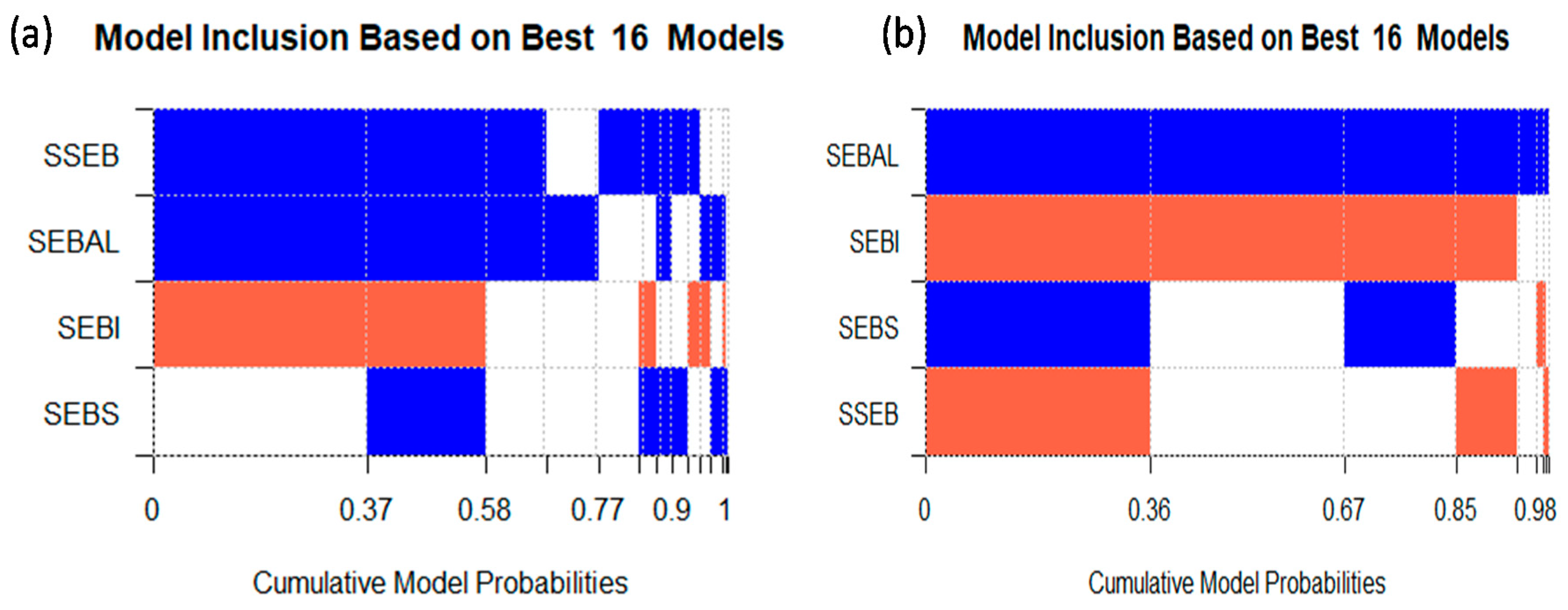
3.2. Effect of Model Priors

Considering the fair and simple reasons in determining the weight of the four SEB models, the uniform model prior was employed before this study for examination. The BMA method assembles four SEB models (i.e., four explanatory variables) thus 2⁴ = 16 combinations and thus 16 models, the 16 models are ranked by their magnitude of posterior model probability (PMP, i.e., the model probability after loading data, contrast to prior model probability without data information) in horizontal axis. As is illustrated in Figure 4, every two coordinate points represent a model (i.e., length of the scale in x-axis represents the magnitude of posterior model probability), and 16 model ranked by their PMPs in x-axis. The y-axis represented four SEB models, blue color corresponded to a positive coefficient, red to a negative and white to a zero coefficient. Take Huailai station for example, the best model with the largest PMP of 0.37, contained positive SSEB, positive SEBAL, negative SEBI, and zero coefficient of SEBS. The second ranked model had a PIP value of 0.21 (difference between 0.58 and 0.37), contained positive SSEB, SEBAL, SEBS and negative SEBI. It can be seen that the SSEB and SEBAL were included most often among the 16 models and were uniformly positive for Huailai station, while SEBI was included less with all negative coefficients but SEBS with all positive coefficient, reflects the SEBI had a poorer performance than SEBS, which was abnormal with the single model performances of Huailai station in Figure 2. The model inclusion for Sidaoqiao station was different from that of Huailai station. The best model with the most mass of 36% model probability took the four SEB models into account but the coefficient sign of the four models changed individually (SEBAL and SEBS were positive, SEBI and SSEB were negative). The SEBAL was included most and had consistently positive coefficients, but SSEB was included least and all coefficients were negative, which was inconsistent with the result of Sidaoqiao station in Figure 3. This result indicated that assigning a uniform model prior yield uncertainty in model selections, i.e., treating each model indiscriminately in weight determination tends to lead to unsatisfactory results without considering single model performance.

The posterior model size distribution in Figure 5 shows how far the posterior distribution distant with the prior distribution. The posterior expected model size became 2.12 at Huailai station and 2.32 at Sidaoqiao station after updating the prior. We can conclude that the best model size is around 2, for it corresponded to the highest posterior inclusion probability (PIP, i.e., the sum of PMPs for all models and represents the importance of each models) in posterior, far greater than that of prior. It is worth noted that the largest model size of 4 in posterior and prior at two stations, merely corresponded to an extremely low PIP, reflected that larger model size may cause poor performance in model prior selection. This result indicated that a higher PIP was yielded around size 2 after updating the prior, and importantly, a size about 2 proved to be the best model size when choosing model priors in other approaches (i.e., fixed, pip and random).

To consider single model performances and other subjective aspects in choosing model priors, we employed three model priors approaches (fixed, pip and random) to address uncertainty in models selection. Figure 6 shows the comparison of the three model prior methods (fixed, PIP, and random) through the values of PIP at two stations. For Huailai station, the horizontal axis indicates that the SEBAL is the most important model because of its substantially higher PIP than the other SEB methods, which is consistent with the result of Figure 2. The random model prior performed better than the PIP and fixed methods with the highest values of PIP (0.881, 0.678, 0.668, and 0.558, respectively). However, the performance of SSEB was relatively unsatisfactory compared with that of SEBS and S-SEBI in the cases of random and fixed. We thought this may be due to both SEBAL and SSEB have an effect of overestimation (as both the regression lines in Figure 2 have a slope greater than 1), therefore SEBI and SEBS (slope of regression lines smaller than 1 and underestimated) have a higher PIP than SSEB in some cases to avoid the overall overestimated result. However, the PIP method of SSEB performed better than SEBS, which was consistent with Figure 2. Similarly, at Sidaoqiao station, the horizontal axis indicates that the SEBAL is still the most important model for its apparent higher PIP, coincidentally, the PIP of three BMA methods nearly approached 1, reflects a better performance than that of Huailai station, which is consistent with the result of Figure 3. The random model prior performed better than the PIP and fixed priors with the highest PIP (1, 0.956, 0.642, and 0.524, respectively). However, the performance of SSEB was poor compared with SEBS and SEBI in the case of fixed and random. This may be because both SEBAL and SSEB had an overestimation effect, thus SEBI and SEBS had a higher level of importance to avoid overall overestimation.

3.3. Performances of the BMA Methods

A comparison of the ET24 values predicted by the three different BMA methods (fixed, PIP, and random) with measured values for Huailai station is shown in Figure 7. In general, any one of them has an apparently superior performance over any single SEB model, with a higher R², substantially lower RMSE, and greater NSE. Taking the random BMA for example, the random BMA had a higher R² (0.750), lower RMSE (0.902 mm/day), and greater NSE (0.746) than the best single SEB model SEBAL, which indicates greater relevance with the measured values, lower deviation, and a higher model performance. The result was within acceptable limits compared with similar research conducted by Zhu et al. [31], in which the R² ranged from 0.49 to 0.80, and NSE ranged from −2.12 to 0.79 when the original parameterization $\beta =1\mathrm{kPa}$. In addition, the regression lines in Figure 7 indicate that the estimation of three BMA models had different characteristics. All of them were found to underestimate compared with the measured values. Moreover, the performance of fixed BMA was basically the same as that of random BMA, with the same R² and NSE, and nearly the same RMSE (0.903 and 0.902). Both the fixed and random BMA performed better than PIP, with a higher R², lower RMSE, and greater NSE. Comparison of the ET24 values predicted by three different BMA methods with measured values for Sidaoqiao station is shown in Figure 8. Each of them surpassed any of the four single SEB models, with a higher R², lower RMSE, and greater NSE. Taking the random BMA for example, the random had a higher R² (0.796), lower RMSE (0.602 mm/day), and greater NSE (0.793) compared with the best single SEB model SEBAL, indicating a higher quality and accuracy of model performance. The result was within an acceptable interval compared with similar research by Zhu [31] either. The regression lines indicated that the estimation of three BMA models have different characteristics. All of them were found to slightly underestimate compared to the measured values. The random BMA had the best performance with the highest R², lowest RMSE and greatest NSE compared with PIP and fixed BMA. In addition, the fixed BMA performed better than PIP with a higher R². In conclusion, the results revealed that the BMA method is greatly superior to choosing any single SEB model at two stations, and the necessity of coupling SEB models with BMA method is significant for its stability and reliability.

The confidence interval of ET24 in the time series was employed to identify the reliability of the simulated ET values obtained by the three BMA methods compared with the measured data, as shown in Figure 9. All measured data points were contained completely by the simulated confidence interval in the three BMA methods, which indicates that all three BMA methods could give an accurate variation range of the ET values. Nevertheless, the dates corresponding to the second peak (i.e., between May 2015 to September 2015) had a relatively poor performance as the maximum simulated values were far from the measured ones. In spite of the similarities shared by the three methods, the detailed differences should not be ignored. The PIP method had a relatively better performance compared with the fixed and random BMA method, as the simulated data around second peak had better accuracy because of the smaller interval at Huailai station. Similarly, at Sidaoqiao station nearly all measured points were included in the simulated variation interval, indicating that the simulated result was satisfactory. The rising and falling trend of the line roughly matched the shape of the shaded area, which reveals that the three simulated BMA methods could provide an accurate variation range of ET24. The performances of the three BMA methods were essentially similar; however, the PIP method might be more accurate for its narrower interval, which is consistent with the result for Huailai station.

4. Conclusions

Four SEB models coupled with the BMA method are investigated in this study, and several points can be concluded from the results of the two stations, namely: first, for single SEB model validation, the SEBAL and SSEB performed better than SEBI and SEBS with higher R², lower RMSE, and greater NSE. Secondly, three BMA methods (i.e., fixed, PIP, and random) were proposed to demonstrate the impacts of the chosen uniform model prior assumption in the process of determining prior expected model size. By comparing their PIP values, we found that SEBAL still demands higher weights because of its higher PIP values. Moreover, SEBAL was included most among the 16 tested models and was uniformly positive, whereas SEBI possessed all negative coefficients and was included relatively less among the 16 best models. The results indicate that the BMA methods had a higher accuracy, smaller bias, and higher reliability than individual SEB methods, suggesting the superiority of the BMA over choosing any single model.

Integration of SEB models by the BMA method in this study has similarities and differences compared to other existing research. Zhu [31] in 2016 integrated four ET models (P-M, S-W, A-A, PT-JPL) using BMA method to predict terrestrial evapotranspiration across north China, and drew a similar conclusion: the BMA yielded a more accurate and reliable prediction than the four individual models. Moreover, Chen [32] in 2015 applied BMA method to merge 8 models (including 5 empirical models) to estimate terrestrial evapotranspiration in China, found that BMA method outperformed the 8 models and fit the measured data better (decreased 4% RMSE compared to the best individual model), which drew a similar conclusion and consistent with our study. However, Yao [14] in 2017 merged three process-based ET models (MOD16, PT-JPL and SEMI-PM) to predict global terrestrial evapotranspiration using the support vector machine (SVM) method, and found that the SVM method outperformed individual models as well as BMA method (improved 10–20% accuracy than individual models and 5–10% than BMA method) by evaluating performances over 200 flux towers sites. Cause of the different conclusions between Yao and our study mainly may be due to the disparity between datasets, which indicates that process-based models coupled with machining learning method (SVM) outperforms the BMA method with enough datasets for training and testing. Process-based models consider processes of energy and moisture exchange as well as transport processes [48], similar to physical-based models which are based on the surface energy balance equation and Monin-Obukhov similarity theory [1]. Whereas empirical models estimate ET through building relationship between inputs and outputs utilizing training data, and not associated with ET process mechanism, these models provide accurate ET estimates as long as all behaviors found within the system are represented by enough training data [14]. Contrast with the long processing time to train a model for empirical-based models, the physical-based models do not require training samples to estimation ET due to well-founded cause-effect relationships of input variables, though the accuracy may not be the highest [14,49].

Landsat 8 satellite data has abundant spectral information, with higher spatial resolution (with a 30 m spatial resolution) than the MODIS satellite (with a 1 km spatial resolution), which was employed for retrieval by Chen [32] (MODIS ASCII satellite data) and Yao [14] (MOD13A2 and MOD13A2), therefore the latest Landsat 8 dataset is an ideal data source for retrieval of evapotranspiration in subsequent researches. A combination of Landsat remote sensing and meteorological data can realize the accurate estimation of evapotranspiration at large spatial scales, integrations for physical-based SEB models by the BMA method can provide an accurate estimation of evapotranspiration over regions with inadequate data (such as semi-arid/arid regions), which is significant in research for the rational utilization and distribution of water resources in arid/semi-arid regions, as well as climate change and agricultural development. Future studies will consider introducing machine learning models (such as SVM and random forest) coupled with physical-based, empirical-based and process-based models, integrated by the BMA method to improve ET estimation over arid or non-arid regions.

Compared with the 56 years data of mean precipitation and pan evaporation, the result has limitations due to the short study period (2014–2015) to some extent. The annual mean precipitation between 2014–2015 years are 426.7 mm of Huailai station and 43.7 mm of Sidaoqiao station, the annual mean pan evaporation are 1460.4 and 2075.7mm respectively, with more precipitation but less evaporation that biased towards wetter conditions in representing long-term averages. It should be noted that the eddy covariance measurements have a significant impact on model performance indirectly, for the measured ET values are maintained from the EC flux tower stations. Obtaining reliable data from EC stations is still a conundrum that has not yet been fully investigated, affected by various factors such as a lack of energy balance closure, the presence of vegetation in the field, distributions of representative source areas, etc., which cause an uncertainty for the measurement of ET [50,51,52]. The BMA method has satisfactorily improved prediction accuracy, and addressed the uncertainty of SEB models when employed for the estimation of ET for cropland in arid/semi-arid regions; whether it is applicable in non-arid areas requires further research. Finally, it is worth mentioning that inherent theoretical limitations still remain for the BMA method. Since the essence of the BMA multi-model ensemble method is a model training method, it is necessary to use the observation data to train and test each simulation model within the model set to determine its BMA coefficient and thus the method is powerless for grid points without corresponding observation data. In brief, the robustness of the BMA method requires more comprehensive research.

References

1. Wang, K.C.; Dickinson, R.E. A Review of Global Terrestrial Evapotranspiration: Observation, Modeling, Climatology and Climatic Variability. Rev. Geophys. 2012, 50, RG2005. [Google Scholar] [CrossRef]
2. Shiklomanov, A.I. World Water Resources: A New Appraisal and Assessment for the Twenty-First Century: A Summary of the Monograph “World Water Resources”; Reports; UNESCO: Paris, France, 1998; 37p. [Google Scholar]
3. Yuan, W.P.; Liu, S.G.; Liang, S.L.; Tan, Z.X.; Liu, H.P.; Young, C. Estimations of Evapotranspiration and Water Balance with Uncertainty over the Yukon River Basin. Water Resour. Manag. 2012, 26, 2147–2157. [Google Scholar] [CrossRef]
4. Liu, Y.; Ye, L.; Qin, H.; Hong, X.; Ye, J.; Yin, X. Monthly streamflow forecasting based on hidden Markov model and Gaussian Mixture Regression. J. Hydrol. 2018, 561, 146–159. [Google Scholar] [CrossRef]
5. Zhang, Y.R.; Sun, A.; Sun, H.W.; Gui, D.W.; Xue, J.; Liao, W.H.; Yan, D.; Zhao, N.; Zeng, X.F. Error adjustment of TMPA satellite precipitation estimates and assessment of their hydrological utility in the middle and upper Yangtze River Basin, China. Atmos. Res. 2019, 216, 52–64. [Google Scholar] [CrossRef]
6. Jung, M.; Reichstein, M.; Ciais, P.; Seneviratne, S.I.; Sheffield, J.; Goulden, M.L. Recent Decline in the Global Land Evapotranspiration Trend Due to Limited Moisture Supply. Nature 2010, 467, 951–954. [Google Scholar] [CrossRef]
7. Sheffield, J.; Wood, E.F.; Roderick, M.L. Little Change in Global Drought Over the Past 60 years. Nature 2012, 491, 435–438. [Google Scholar] [CrossRef] [PubMed]
8. Yan, D.; Jia, Z.W.; Xue, J.; Sun, H.W.; Gui, D.W.; Liu, Y.; Zeng, X.F. Inter-Regional Coordination to Improve Equality in the Agricultural Virtual Water Trade. Sustainability 2018, 10, 4561. [Google Scholar] [CrossRef]
9. Ma, W.Q.; Ma, Y.M.; Ishikawa, H. Evaluation of the SEBS for upscaling the evapotranspiration based on in-situ observations over the Tibetan Plateau. Atmos. Res. 2014, 138, 91–97. [Google Scholar] [CrossRef]
10. Xue, J.; Gui, D.; Lei, J.; Sun, H.; Zeng, F.; Mao, D.; Zhang, Z.; Jin, Q.; Liu, Y. Oasis microclimate effects under different weather events in arid or hyper arid regions: A case analysis in southern Taklimakan desert and implication for maintaining oasis sustainability. Theor. Appl. Climatol. 2018, 8, 1–13. [Google Scholar] [CrossRef]
11. Yin, J.; Zhan, C.S.; Ye, W. An Experimental Study on Evapotranspiration Data Assimilation Based on the Hydrological Model. Water Resour. Manag. 2016, 30, 5263–5279. [Google Scholar] [CrossRef]
12. Guo, D.; Westra, S.; Maier, H.R. An R package for modelling actual, potential and reference evapotranspiration. Environ. Model. Softw. 2016, 78, 216–224. [Google Scholar] [CrossRef]
13. McMahon, T.A.; Finlayson, B.L.; Peel, M.C. Historical developments of models for estimating evaporation using standard meteorological data. WIREs Water 2016, 3, 788–818. [Google Scholar] [CrossRef]
14. Yao, Y.; Liang, S.; Li, X.; Chen, J.; Liu, S.; Jia, K.; Zhang, X.; Xiao, Z.; Fisher, J.B.; Mu, Q.; et al. Improving global terrestrial evapotranspiration estimation using support vector machine by integrating three process-based algorithms. Agric. For. Meteorol. 2017, 242, 55–74. [Google Scholar] [CrossRef]
15. Fisher, J.B.; Tu, K.P.; Baldocchi, D.D. Global Estimates of the Land-atmosphere Water Flux Based on Monthly AVHRR and ISLSCP-II data, Validated at 16 FLUXNET Sites. Remote Sens. 2008, 112, 901–919. [Google Scholar] [CrossRef]
16. Fisher, J.B.; Malhi, Y.; Bonal, D.; Da Rocha, H.R.; De Araujo, A.C.; Gamo, M.; Goulden, M.L.; Hirano, T.; Huete, A.R.; Kondo, H.; et al. The Land-atmosphere Water Flux in the Tropics. Glob. Chang. Biol. 2009, 15, 2694–2714. [Google Scholar] [CrossRef]
17. Badgley, G.; Fisher, J.B.; Tu, K.P.; Vinukollu, R.K. On Uncertainty in Global Evapotranspiration Estimates from Choice of Input Forcing Datasets. Hydrometeorology 2015, 16, 1449–1455. [Google Scholar] [CrossRef]
18. Verma, M.; Fisher, J.B.; Mallick, K.; Ryu, Y.; Kobayashi, H.; Guillaume, A.; Moore, G.; Ramakrishnan, L.; Hendrix, V.; Wolf, S.; et al. Global Daily Surface Net-radiation at 5 km from MODIS. Remote Sens. 2016, 8, 739. [Google Scholar] [CrossRef]
19. Lian, J.J.; Huang, M.B. Evapotranspiration Estimation for an Oasis Area in the Heihe River Basin Using Landsat-8 Images and the METRIC Model. Water Resour. Manag. 2015, 29, 5157–5170. [Google Scholar] [CrossRef]
20. Cleugh, H.A.; Leuning, R.; Mu, Q.; Running, S.W. Regional evaporation estimates from flux tower and MODIS satellite data. Remote Sens. Environ. 2007, 106, 285–304. [Google Scholar] [CrossRef]
21. French, A.N.; Hunsaker, D.J.; Thorp, K.R. Remote sensing of evapotranspiration over cotton using the TSEB and METRIC energy balance models. Remote Sens. Environ. 2015, 158, 281–294. [Google Scholar] [CrossRef]
22. Sun, H.; Gui, D.; Yan, B.; Liu, Y.; Liao, W.; Zhu, Y.; Lu, C.; Zhao, N. Assessing the potential of random forest method for estimating solar radiation using air pollution index. Energy Convers. Manag. 2016, 119, 121–129. [Google Scholar] [CrossRef] [Green Version]
23. Roula, B.; Inga, M.; Andres, M.; Ticlavilca, W.R. Wavelet-Multivariate Relevance Vector Machine Hybrid Model for Forecasting Daily Evapotranspiration. Stoch. Environ. Res. Risk Assess. 2016, 30, 103–117. [Google Scholar] [CrossRef]
24. Dormann, C.F.; Calabrese, J.M.; Guillera-Arroita, G.; Matechou, E. Model averaging in ecology: A review of Bayesian, information-theoretic, and tactical approaches for predictive inference. Ecol. Monogr. 2018, 88, 485–504. [Google Scholar] [CrossRef]
25. Raftery, A.E.; Gneiting, T.; Balabdaoui, F.; Polakowski, M. Using Bayesian Model Averaging to Calibrate Forecast Ensembles. Mon. Weather Rev. 2005, 133, 1155–1174. [Google Scholar] [CrossRef] [Green Version]
26. Duan, Q.; Ajami, N.K.; Gao, X.; Sorooshian, S. Multi-model Ensemble Hydrologic Prediction Using Bayesian Model Averaging. Adv. Water Resour. 2007, 30, 1371–1386. [Google Scholar] [CrossRef]
27. Ellison, A.M. Bayesian Inference in Ecology. Ecol. Lett. 2004, 7, 509–520. [Google Scholar] [CrossRef]
28. Vrugt, J.A.; Robinson, B.A. Treatment of Uncertainty Using Ensemble Methods: Comparison of Sequential Data Assimilation and Bayesian Model Averaging. Water Resour. Res. 2007, 43, W01411. [Google Scholar] [CrossRef]
29. Liu, Y.; Xue, J.; Gui, D.; Lei, J.; Sun, H.; Lv, G.; Zhang, Z. Agricultural Oasis Expansion and Its Impact on Oasis Landscape Patterns in the Southern Margin of Tarim Basin, Northwest China. Sustainability 2018, 10, 1957. [Google Scholar] [CrossRef]
30. Liang, Z.M.; Wang, D.; Guo, Y.; Zhang, Y.; Dai, R. Application of Bayesian Model Averaging Approach to Multi-Model Ensemble Hydrologic Forecasting. J. Hydrol. Eng. 2011, 18, 1426–1436. [Google Scholar] [CrossRef]
31. Zhu, G.F.; Li, X.; Zhang, K.; Ding, Z.Y. Multi-model Ensemble Prediction of Terrestrial Evapotranspiration Across North China Using Bayesian Model Averaging. J. Hydrol. Process. 2016, 30, 2861–2879. [Google Scholar] [CrossRef]
32. Chen, Y.; Yuan, W.P.; Xia, J.Z.; Joshua, B. Fisher, Using Bayesian Model Averaging to Estimate Terrestrial Evapotranspiration in China. J. Hydrol. 2015, 52, 537–549. [Google Scholar] [CrossRef]
33. Allen, R.; Tasumi, M.; Trezza, R. Satellite-Based Energy Balance for Mapping Evapotranspiration with Internalized Calibration (METRIC)-Model. J. Irrig. Drain. Eng. 2007, 133, 380–394. [Google Scholar] [CrossRef]
34. Bastiaanssen, W.G.M.; Menenti, M.; Feddes, R.A.; Holtslag, A.A.M. A Remote Sensing Surface Energy Balance Algorithm for Land (SEBAL). J. Hydrol. 1998, 212, 198–212. [Google Scholar] [CrossRef]
35. Allen, R.; Tasumi, M.; Morse, A.; Trezza, R.; Wright, J.; Bastiaanssen, W.; Kramber, W.; Lorite, I.; Robison, C. Satellite-Based Energy Balance for Mapping Evapotranspiration with Internalized Calibration (METRIC)-Applications. J. Irrig. Drain. Eng. 2007, 133, 395–406. [Google Scholar] [CrossRef]
36. Senay, G.B.; Budde, M.E.; Verdin, J.P. Enhancing the Simplified Surface Energy Balance (SSEB) Approach for Estimating Landscape ET: Validation with the METRIC Model. Agric. Water Manag. 2011, 98, 606–618. [Google Scholar] [CrossRef]
37. Roerink, G.J.; Su, Z.; Menenti, M. S-SEBI: A Simple Remote Sensing Algorithm to Estimate the Surface Energy Balance. Phys. Chem. Earth 2000, 25, 147–157. [Google Scholar] [CrossRef]
38. Su, Z.; Schmugge, T.; Kusts, W.P. An Evaluation of Two Models for Estimation of the Roughness Height for Heat Transfer between the Land Surface and Atmosphere. J. Appl. Meteorol. 2001, 40, 1933–1951. [Google Scholar] [CrossRef]
39. Su, Z. The Surface Energy Balance System (SEBS) for Estimation of Turbulent Heat Fluxes. Hydrol. Earth Syst. Sci. 2002, 6, 85–99. [Google Scholar] [CrossRef]
40. Hoeting, J.A.; Madigan, D.; Raftery, A.E.; Volinsky, C.T. Bayesian Model Averaging: A Tutorial. Stat. Sci. 1999, 14, 382–417. [Google Scholar]
41. Ley, E.; Steel, M.F. On the Effect of Prior Assumptions in Bayesian Model Averaging with Applications to Growth Regressions. J. Appl. Econom. 2009, 24, 651–674. [Google Scholar] [CrossRef]
42. Legates, D.R.; McCabe, G.J. Evaluating the Use of ‘goodness-of-fit’ Measures in Hydrologic and Hydroclimatic Model Validation. Water Resource. Res. 1999, 35, 233–241. [Google Scholar] [CrossRef]
43. Jackson, R.D. Estimation of daily evapotranspiration from one time-day measurements. Agric. Water Manag. 1983, 7, 351–362. [Google Scholar] [CrossRef]
44. Tian, F.; Qiu, G.; Yang, Y.; Lü, Y.; Xiong, Y. Estimation of evapotranspiration and its partition based on an extended three-temperature model and MODIS products. J. Hydrol. 2013, 498, 210–220. [Google Scholar] [CrossRef]
45. Baldocchi, D.; Falge, E.; Gu, L.; Olson, R.; Hollinger, D.; Running, S. FLUXNET: A New Tool to Study the Temporal and Spatial Variability of Ecosystem-scale Carbon Dioxide, Water Vapor and Energy Flux Densities. Bull. Am. Meteorol. Soc. 2001, 82, 2415–2434. [Google Scholar] [CrossRef]
46. Ke, Y.; Im, J.; Park, S.; Gong, H. Downscaling of MODIS One Kilometer Evapotranspiration Using Landsat-8 Data and Machine Learning Approaches. Remote Sens. 2016, 8, 215. [Google Scholar] [CrossRef]
47. Bhattarai, N.; Mallick, K.; Brunsell, N.A.; Sun, G.; Jain, M. Evapotranspiration from An Image-Based Implementation of the Surface Temperature Initiated Closure(STIC1.2) Model and Its Validation across an Aridity Gradient in the Conterminous US. Hydrol. Earth Syst. Sci. 2018, 22, 2311–2341. [Google Scholar] [CrossRef]
48. Vinukollu, R.K.; Wood, E.F.; Ferguson, C.R.; Fisher, J.B. Global estimates of evapotranspiration for climate studies using multi-sensor remote sensing data: Evaluation of three process-based approaches. Remote Sens. Environ. 2011, 115, 801–823. [Google Scholar] [CrossRef]
49. Verrelst, J.; Rivera, J.P.; Veroustraete, F. Experimental Sentinel-2 LAI estimation using parametric, non-parametric and physical retrieval methods—A comparison. ISPRS J. Photogramm. Remote Sens. 2015, 108, 260–272. [Google Scholar] [CrossRef]
50. Wang, J.M.; Zhuang, J.X.; Wang, W.Z.; Liu, S.M.; Xu, Z.W. Assessment of Uncertainties in Eddy Covariance Flux Measurement Based on Intensive Flux Matrix of HiWATER-MUSOEXE. IEEE Geosci. Remote Sens. 2014, 12, 259–263. [Google Scholar] [CrossRef]
51. Masseroni, D.; Corbari, C.; Mancini, M. Validation of theoretical footprint models using experimental measurements of turbulent fluxes over maize fields in PoValley. Environ. Earth Sci. 2014, 72, 1213–1225. [Google Scholar] [CrossRef]
52. Masseroni, D.; Corbari, C.; Mancini, M. Limitations and improvements of the energy balance closure with reference to experimental data measured over a maize field. Atmósfera 2014, 27, 335–352. [Google Scholar] [CrossRef] [Green Version]
Figure 1. Locations of the two study areas: (a) Sidaoqiao station in Nei Mongol Autonomous Region; (b) Huailai station in Hebei province. The colored map of China represents the spatial distribution of annual average precipitation (mm/year) over China. The pentagram sign indicates specific locations of two flux stations.
Atmosphere 10 00188 g001
Figure 2. Comparison of ET24 values predicted from the SEB models with measured values at Huailai station: (a) comparison of ET predicted from SEBAL with measured, (b) comparison of ET predicted from SSEB with measured, (c) comparison of ET predicted from SEBI with measured, and (d) comparison of ET predicted from SEBS with measured. The red dotted lines represent a slope of 1 (i.e., the predicted value equals to the measured).
Atmosphere 10 00188 g002
Figure 3. Comparison of ET24 values predicted from the SEB models with measured values at Sidaoqiao station: (a) comparison of ET predicted from SEBAL with measured, (b) comparison of ET predicted from SSEB with measured, (c) comparison of ET predicted from SEBI with measured, and (d) comparison of ET predicted from SEBS with measured. The red dotted lines represent a slope of 1 (i.e., the predicted value equals to the measured).
Atmosphere 10 00188 g003
Figure 4. Model inclusion based on the best 16 models of uniform model priors at two stations: (a) Huailai station; (b) Sidaoqiao station. The y-axis represents four SEB models, the 16 model are ranked by their PMPs in x-axis. Blue color corresponds to a positive coefficient, red to a negative, and white to a zero coefficient.
Atmosphere 10 00188 g004
Figure 5. Comparison of the model size distribution for uniform model prior at two stations: (a) Huailai station; (b) Sidaoqiao station. The x-axis represents model size included, y-axis represents values of PIP. It should be noted that the posterior expected model size is equal to the sum of the PIPs.
Atmosphere 10 00188 g005
Figure 6. Comparison of the values of PIP of four SEB models under three model priors (BMA-fixed, BMA-PIP and BMA-random) at two stations: (a) Huailai station; (b) Sidaoqiao station.
Atmosphere 10 00188 g006
Figure 7. Comparison of ET24 values predicted by three different BMA methods with measured values for Huailai station: (a) BMA-fixed, (b) BMA-PIP, and (c) BMA-random. The red dotted lines represent a slope of 1 (i.e., the predicted value equals to the measured).
Atmosphere 10 00188 g007
Figure 8. Comparison of ET24 values predicted by three different BMA methods with measured values for Sidaoqiao station: (a) BMA-fixed, (b) BMA-PIP, and (c) BMA-random. The red dotted lines represent a slope of 1 (i.e., the predicted value equals to the measured).
Atmosphere 10 00188 g008
Figure 9. Comparison of the confidence interval of ET24 values in time series by three different BMA methods with measured values at two stations: (ac) for Huailai station; (df) Sidaoqiao station. The shaded area represents the range of the ET values derived from the BMA methods, with a confidence of 90%, and the black solid line represents the measured ET value, from 14 January 2014 to 31 October 2015.
Atmosphere 10 00188 g009