Anthropogenic CH₄ Emissions in the Yangtze River Delta Based on A “Top-Down” Method

Abstract

There remains significant uncertainty in the estimation of anthropogenic CH₄ emissions at local and regional scales. We used atmospheric CH₄ and CO₂ concentration data to constrain the anthropogenic CH₄ emission in the Yangtze River Delta one of the most populated and economically important regions in China. The observation of atmospheric CH₄ and CO₂ concentration was carried out from May 2012 to April 2017 at a rural site. A tracer correlation method was used to estimate the anthropogenic CH₄ emission in this region, and compared this “top-down” estimate with that obtained with the IPCC inventory method. The annual growth rates of the atmospheric CO₂ and CH₄ mole fractions are 2.5 ± 0.7 ppm year⁻¹ and 9.5 ± 4.7 ppb year⁻¹, respectively, which are 9% and 53% higher than the values obtained at Waliguan (WLG) station. The average annual anthropogenic CH₄ emission is 4.37 (± 0.61) × 10⁹ kg in the YRD (excluding rice cultivation). This “top-down” estimate is 20–70% greater than the estimate based on the IPCC method. We suggest that possible sources for the discrepancy include low biases in the IPCC calculation of emission from landfills, ruminants and the transport sector.

1. Introduction

The source apportionment of CH₄ is important for the study of carbon cycle and climate change. The mole fraction of CH₄ in the atmosphere increased by 157% from 1750 to 2011 [1,2]. As the second largest greenhouse gas next to CO₂, CH₄ has a warming potential of 28 times that of CO₂ with a 100-year time horizon [2]. In addition to the greenhouse effect, CH₄ also affects the chemical and photochemical reactions in the atmosphere [3]. The annual growth rate of atmospheric CH₄ was 6.9 ± 2.4 ppb year⁻¹ from 2007 to 2017 [4]. However, the source contributions of CH₄ have so far not been accurately quantified, especially at the regional and the city scale [5].

Anthropogenic CH₄ emissions account for 50–65% of the global CH₄ emissions of 5.82 (± 0.5) × 10¹¹ kg year⁻¹ [6,7]. Large uncertainties still exist in regional anthropogenic emission estimates. These estimates are usually based on the Intergovernmental Panel on Climate Change (IPCC) inventory method. The IPCC method aggregates the CH₄ emissions generated by different anthropogenic activities and sums up the individual components to the domain of interest. One problem is that activity data, such as landfill and livestock, and emission factors cannot be accurately determined at the regional and the city scale [8,9,10]. A study in Beijing found that the uncertainty caused by landfill accounts for nearly half of the total uncertainty in the CH₄ emission estimate [11]. Accurate and timely calculations of anthropogenic CH₄ emissions at the regional scale are necessary for assessing the effectiveness of emission reduction policies.

Anthropogenic greenhouse gas emissions can also be estimated from observations of the gaseous concentrations in the atmosphere (“top-down” methods). The “atmospheric method” used in this study is one of the “top-down” approaches. One reason for using the atmospheric method is that many sources of anthropogenic CH₄ cannot be quantified with traditional methods, such as the chamber method [12,13,14]. The atmospheric method requires simultaneous concentration measurements of the target gas (CH₄) and a tracer gas (usually CO₂) when there is no disturbance from sinks or other natural sources [15]. In an observational study using aircraft profile measurement over a broad region of Alaska and Canada, the concentrations of CH₄ and CO₂ increase synchronously with height, showing a strong positive correlation between the two gases [16]. A similar positive relationship also exists in the surface air in a moderately polluted urban atmosphere of Boulder, USA [16]. The explanation for the positive relationship is that the two gases share common source areas and undergo the same long-range transport [17,18]. The concentration ratio between the two gases were used to estimate the CH₄ emissions in the densely populated urban areas in Southern California, showing that inventory CH₄ emission estimates for these urban areas are lower in comparison to the “top-down” atmospheric estimate [19]. In a study of anthropogenic CH₄ emissions in the Los Angeles megacity, a ground-based remote sensing concentration measurement with 29 different surface targets was used to spatially resolve CH₄:CO₂ emission ratio, once again relying on the linear relationship between the two gaseous concentrations [20].

The atmospheric method is based on a strong correlation between the observed concentration values of two relatively inert gases CH₄ and CO₂. Because the lifetime of these two gases in the atmosphere (7–11 years and 50–200 years, respectively) [21] is much longer than hourly time scales at which the observations are made, the linear slope value of the regression is essentially equivalent to the ratio of their anthropogenic emission strengths. In the applications cited above, the CH₄ emission flux is computed as the product of the concentration regression slope and the anthropogenic CO₂ emission flux, the latter of which can be obtained reliably with the IPCC inventory method [22].

The atmospheric method has been used to track emissions of other gas species besides CH₄. This method was used to infer anthropogenic Hg emissions in Northeast USA, with wintertime Hg and CO₂ concentration data and CO₂ as the tracer [23]. Simultaneous observations of the CO₂ and CO concentrations in a suburban site outside Beijing was used to determine the efficiency of fossil fuel combustion [24]. The concentrations of CO₂ and CO observed in the Asian outflow air combined with a three-dimensional global chemical transport model were used to quantify CO₂ emissions in East Asia [25].

In this paper, we report long-term (five years), near-continuous, and simultaneous observations of atmospheric CH₄ and CO₂ at a lake site near Wuxi, Jiangsu Province, China. Our main objective was to quantify the CH₄ emission in the Yangtze River Delta (YRD) and its interannual variability, using the atmospheric tracer method described above. The second objective was to evaluate the validity of the CH₄ emissions calculated with the “bottom-up” IPCC inventory method against the atmospheric or “top-down” emission estimates.

2. Experiments

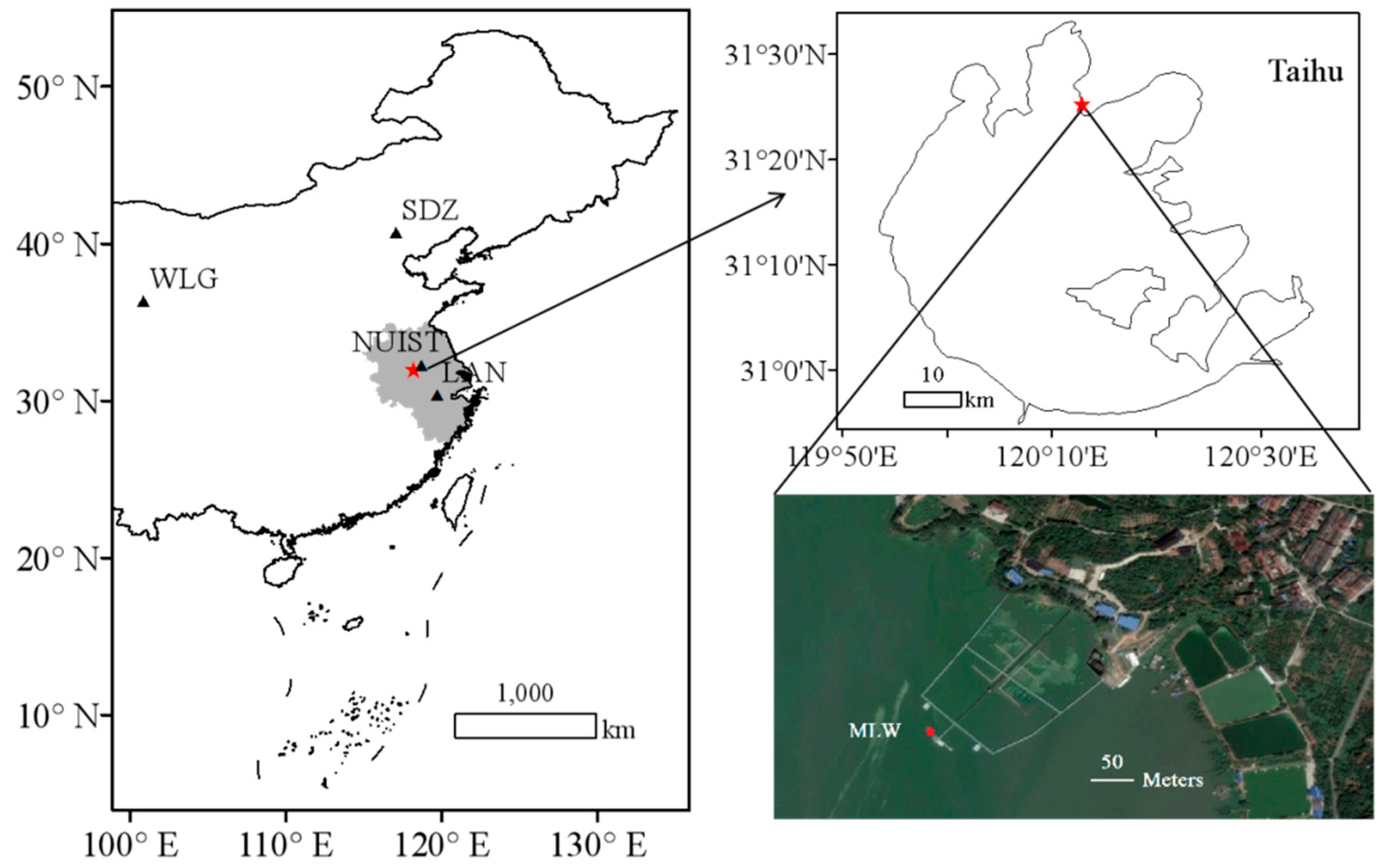
2.1. Study Area and Observational Site

The YRD in East China occupies only 2.1% of the land area of China (including Jiangsu Province, Zhejiang Province, Anhui Province and Shanghai), but contributes 1/4 of the total economic output [26]. The Wuxi Municipality is located roughly in the middle of the Yangtze River Delta, with a population of about 5 million. Other major cities in this region are Shanghai, Nanjing, Hangzhou, Ningbo and Hefei.

The observational site is located at the Taihu Lake Ecosystem Observatory of the Chinese Academy of Sciences (31.4197° N, 120.2139° E) in Wuxi. Measurements of the CO₂ and CH₄ concentrations were made on a platform about 200 m from the north shore of the lake (Figure 1). The platform was once also part of the Lake Taihu Eddy Flux Network (site id MLW) [27]. The site is surrounded by water, scattered farmlands and residential buildings. The closest traffic road is about 10 km away. The prevailing wind is northwesterly in the winter (Figure S1) and southerly in the summer. In the winter season, the landscape upwind is mostly rural (Figure S1).

2.2. Trace Gas Analyzer

The analyzer we used was based on wavelength scanning cavity ring-down spectroscopy (model G1301 from 14 May 2012 to 6 July 2013 and model G2301 from 20 October 2013 until now, Picarro Inc., Sunnyvale, CA, USA). The measurement frequency is 1 Hz (sampling rate) and the precision (5-s mean) is 0.15 ppm for CO₂ and 1 ppb for CH₄. The air inlet is placed at a height of 3.5 m above the water surface. The water vapor concentration measured by the instrument was used to remove the water vapor dilution effect so the concentrations of CH₄ and CO₂ are expressed as molar ratio of CH₄ or CO₂ to dry air.

The observation period in this study was from May 2012 to April 2017. A large data gap occurred between July and October 2013 owing to instrument malfunction. In the second half of 2016, some data were lost because of loss of power on the platform.

The data from the analyzer were averaged to half-hour intervals. Standard deviation in half an hour and a five-point moving average method with a threshold of 1.5 times the standard deviation were used to filter the outliers. The daily average was achieved when daily data exceeded 75%.

For model G1301, the CO₂ and CH₄ measurements were calibrated twice (2 May 2012 and 22 June 2012) and the details can be found in the supplementary materials of a previously published paper [28]. Model G2301 was calibrated three times on 11 September 2013, 4 November 2015 and 25 August 2016, respectively. The mole fractions of CO₂ and CH₄ were calibrated against two standard CO₂ gases (concentration: 490 ppm or 491 ppm and 385 ppm, National Primary Standard prepared by the National Institute of Meteorology (NIM), China) and two standard CH₄ gases (2.02 ppm and 3.05 ppm or 3.52 ppm, National Primary Standard) each time. The relative error is 0.62–0.37% for CO₂ and 0.81–0.41% for CH₄. We used a dew-point generator (model 610, LI-COR, Inc., Lincoln, NE, USA) to correct the analyzers humidity measurement. The humidity level of the air coming out of the dew-point generator was regulated at five levels and measurement at each humidity level lasted 15 min. The first several minutes when the measurement was transitional were excluded from the analysis. A linear regression fit generated from saturation vapor mixing ratio and observed vapor mixing ratio resulted in a slope value of 0.97–0.99.

No standards were available for us to trace our calibration gases to the WMO scale. NIM participated in two inter-agency comparison experiments on calibration standards including standards traceable to the WMO scale. The results can be found in references [29,30].

2.3. The IPCC Inventory Calculation

The IPCC emissions inventory is a “bottom-up” approach. It takes emission activity data from different economic sectors into account and multiplies them by the corresponding emission factors to estimate the emission. The activity data used in this study were obtained from China Energy Statistical Yearbook [31,32,33,34], China Statistical Yearbook [35,36,37,38], China Rural Statistical Yearbook [39,40,41,42], Jiangsu Statistical Bureau, Auhui Statistical Bureau, Zhejiang Statistical Bureau, Shanghai Statistical Bureau and Wuxi Statistical Bureau. The data on crop straw burning were derived from crop yields combined with grain-to-straw ratio [43]. The data on firewood usage from 1991 to 2006 were estimated with the ratio of firewood usage in the YRD combined with the total firewood usage [44]. Then a time-varying line of the firewood usage was fitted to estimate the 2012–2015 firewood usage in the YRD. We used the default emission factors provided by IPCC if no domestic values are available, such as industry energy consumption, industry processes and livestock. CH₄ emissions from landfills were based on the first order decay model provided by IPCC, taking into account local climatic conditions, the landfill waste volume, organic carbon content and waste age [11,45,46]. CH₄ emissions from rice paddies accounted for different varieties of rice acreage and the corresponding growth period [47,48,49]. The proportion of open-pit mining to the total mining volume has increased year by year in the YRD region [50]. The CH₄ fugitive emissions in the YRD mainly come from coal mining in Xuzhou in Jiangsu Province and Huainan, Huaibei, Fuyang, etc. in Anhui Province. The remaining emission factors for other sectors not listed here were obtained from the relevant literature [51,52].

The Monte Carlo method [52,53] was used to obtain uncertainty ranges of the inventory calculations. The uncertainties of the IPCC method arise from the choice of emission factors and from uncertainties in the activity data. These uncertainties were assumed to follow uniform distributions. The range of variations of the emission factors were given by IPCC or domestic values. For the activity data, an uncertainty range of 10% was assumed. A total of 400,000 ensemble members were calculated to determine a probability distribution function and estimate the emission uncertainties. A 95% confidence interval was used to quantify the random errors.

The CO₂ inventory is well quantified and with less uncertainty. For example, in Austria, Norway, the Netherlands, the UK and the USA, the uncertainty of CO₂ emission factors and activity data for main sources is between ± 0.5% and ± 7% of the means [54]. In comparison, the uncertainty of the CH₄ factors sector is ± 20% to ± 50% of the means [54]. The overall uncertainty of the CO₂ emission estimates is 2–4%, much smaller than that of CH₄ (17–48%) or N₂O (34–230%) [54,55,56].

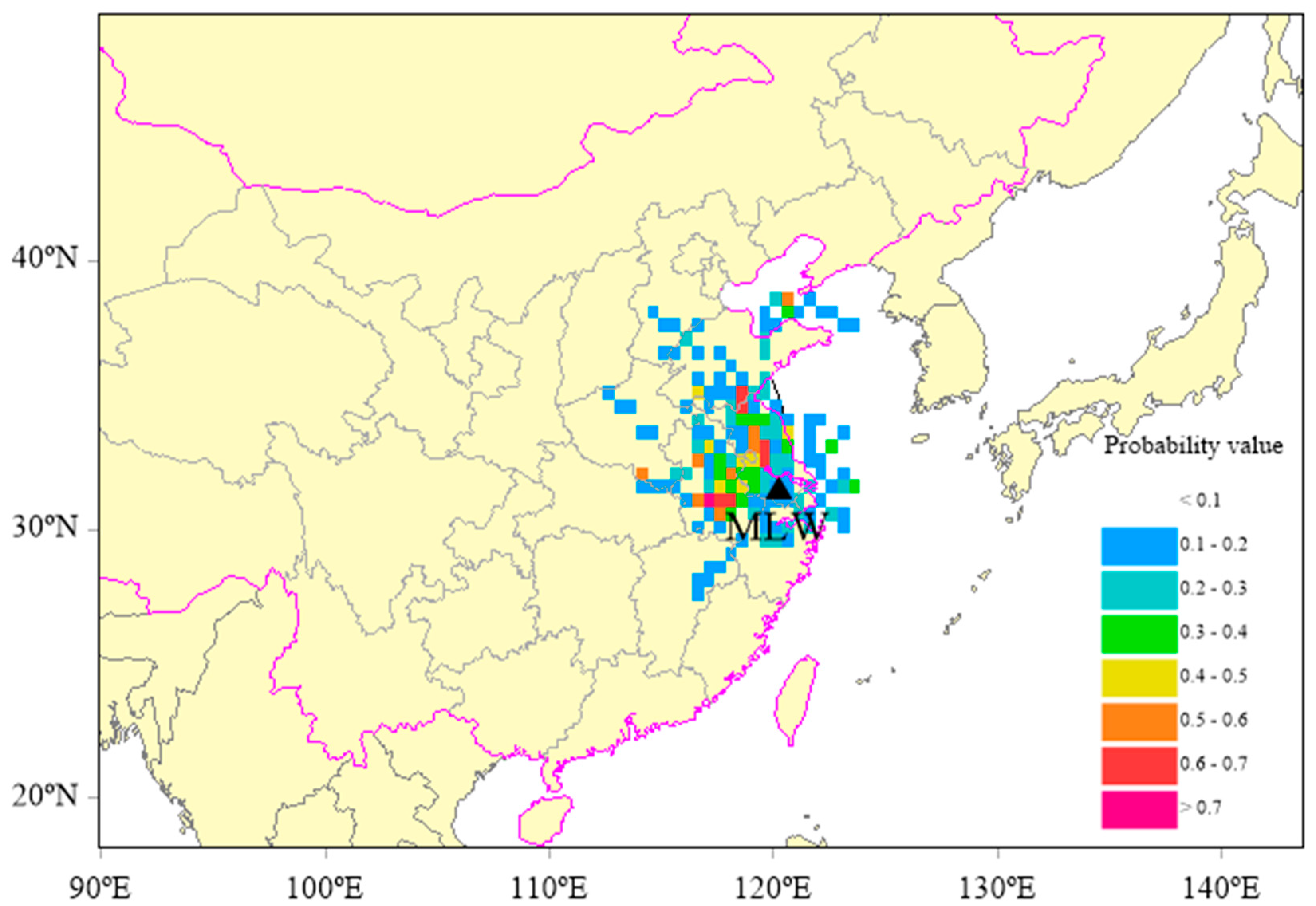
2.4. Application of the Atmospheric Method

We used a geometric mean regression to determine the slope of the CH₄ molar mixing ratio against the CO₂ molar mixing ratio. Because uncertainties exist in both CO₂ and CH₄ concentration measurements, geometric mean regression gives more robust parameter estimates than the ordinary least squares regression [57]. Moreover, there is slight variations between the four seasons according to the national level fuel consumption [58], so we focused on wintertime (December to February inclusive) measurements because plant photosynthesis is minimal and atmospheric CO₂ variations are driven primarily by anthropogenic sources. The annual anthropogenic CH₄ emission flux is the product of the regression slope in winter and the anthropogenic CO₂ flux derived from the IPCC inventory method. We refer to this flux as the “top-down” estimate.

The uncertainty of the atmospheric method comes from two aspects. The first is a result of the regression procedure, and is characterized by the standard deviation of the regression estimate of the geometric mean slope. The second source of uncertainty is caused by the anthropogenic CO₂ emission calculation using the IPCC method. The overall uncertainty of the atmospheric CH₄ emission estimate was calculated with the Monte Carlo method that combines these two sources of uncertainty.

The daytime CO₂ and CH₄ concentrations are indicative of source contributions at the regional scale if there are no direct nearby emissions. This is because the daytime atmospheric boundary layer (ABL) is well mixed and there is no nearby direct emission disturbance. At a suburban site in Xiamen in southeastern China, the vertical profile of CO₂ concentration shows little variation with altitude (below 350 m) between 8:40 and 15:45 [59]. At the Zotino Tall Tower Observatory, CO₂ and CH₄ in the atmosphere becomes well-mixed and their concentrations become nearly indistinguishable at six height levels (4, 52, 92, 157, 227 and 301 m) during day in summer [60]. The ABL height at the MLW site in the winters of 2014–2016, simulated with the Meteoinfo open-source software [61], varies between 570 m and 970 m in the midday period (10:00–17:00; Figure 2). The Meteoinfo program used the Data Assimilation System (GDAS1) as input data, and the predicted ABL height was interpolated spatially to the MLW site. The analysis of Potential Source Contribution Function (PSCF) calculated with the HYSPLIT trajectory model with the 500-m height, the approximate mean height of the mid-point of the ABL, as the end point is shown in Figure 3. The PSCF value can be interpreted as the conditional probability for the specific grid cell, or the ratio of the number of endpoints falling in the grid cell with high concentration (>85th percentile concentration at the receptor site) to the total number of endpoints falling in the grid cell. Grid points having high PSCF values are likely to be potential source regions contributing to the observed concentrations [62]. A weighting function was introduced to deal with the bias brought by PSCF value when the number of endpoints falling in the grid cell was small. The choice of the function was set according to that reported by Sigler and Lee [63]. The calculation was performed for December 2014 with 48-h backward trajectories at 10:00, 13:00 and 16:00 LST each day. In Figure 3, the area with the PSCF value greater than the typical threshold of 0.1 [51,64] is 3.8 × 10⁵ km², of which 76% fall in the political boundary of the YRD. As a result, the daytime observational data at the MLW site can represent the source signatures of the YRD, consistent with a similar study conducted in Nanjing [51].

The footprint analysis revealed the source region mostly likely to have impacted the daytime measurement at MLW. The actual probability value, or weighting factor, was not used later when we aggregated the inventory emission data to the whole YRD region.

At night (23:00–05:00), an inversion layer typically prevails near the ground surface, with high atmospheric stability. The mean height of the boundary layer is 260 m (Figure 2). Because of the strong stability, the CO₂ and CH₄ emitted by anthropogenic sources are trapped near the surface. The lack of mixing implies that the source areas of the observed concentration may span only several kilometers [65]. In other words, the regression slope represents more the emission ratio of local sources than the emission ratio of regional sources, although the exact spatial representation of nighttime observations needs to be further studied.

3. Results

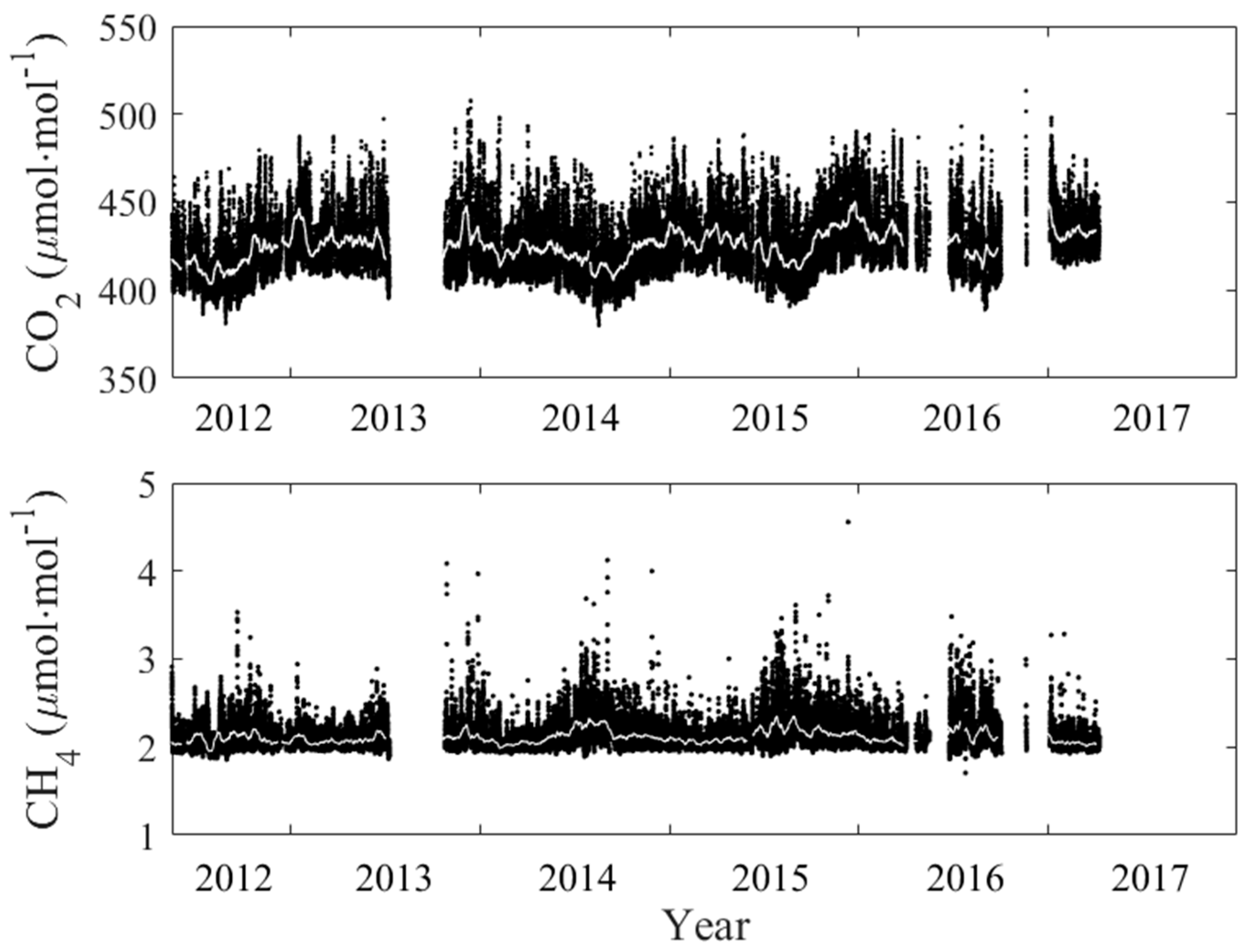
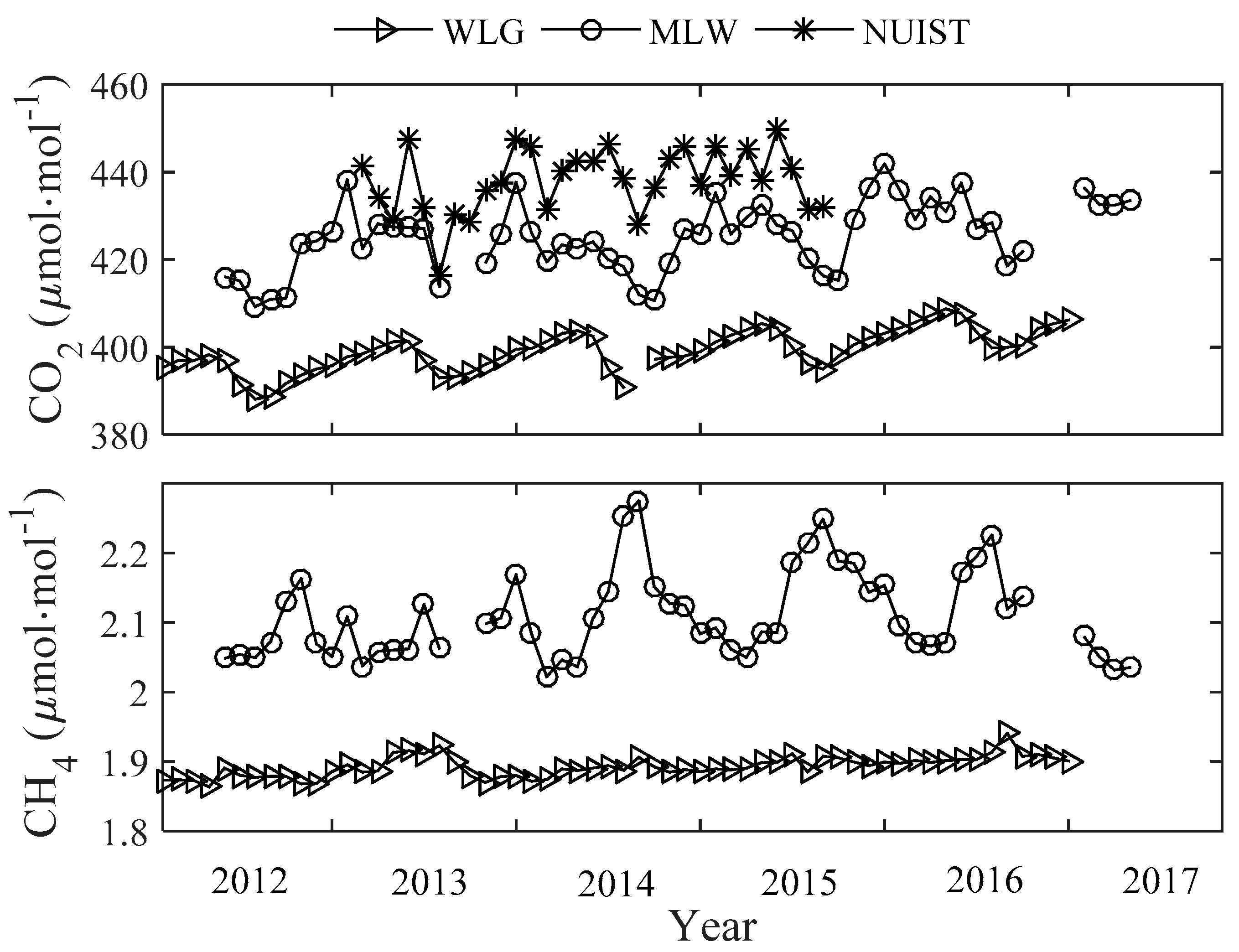
3.1. Temporal Variations of CO₂ and CH₄ Concentrations

Figure 4 shows the temporal variations of half-hourly atmospheric CH₄ and CO₂ mole fractions during the observation period. The data show significant periodic fluctuations through the 24-h cycle, especially for CO₂. Data for 2014 and 2015 are nearly gap-free and are representative of seasonal variations.

Figure 5 shows the diurnal composite concentrations for each of the four seasons in 2014. The diurnal variations of CO₂ and CH₄ show similar patterns in all seasons. In the spring (March, April and May) and autumn (June, July and August), the peaks appear at about 07:00 and the troughs appear at around 17:00. In the summer, the peaks occur at 04:00 and the minimum still appear around 17:00. In the winter (December, and January and February in the next year), the diurnal variations are gentler than in the other three seasons.

Figure 6 shows a comparison of our monthly mean CO₂ and CH₄ concentrations with those observed at Nanjing University of Information Science and Technology (NUIST; 32.20° N, 118.72° E), about 170 km to the northwest of the MLW site. The concentrations observed during the same time period at Mt. Waliguan (WLG, 36.28° N, 100.90° E, 3810 m above the mean sea level), a WMO baseline station representing the background atmosphere for Asia, are also shown [66,67]. NUIST is located at the outskirt of Nanjing, surrounded by residential areas and traffic roads and in the vicinity of two industrial complexes [68]. The atmospheric CO₂ molar fraction is highest at NUIST, followed by MLW and lowest at WLG. Among the three sites, the strongest seasonality of the atmospheric CO₂ molar fraction occurs at the MLW site, with low values in the summer and high values in the winter. The atmospheric CH₄ molar fraction at the MLW site shows an opposite seasonality to CO₂, with high values in the summer and low values in the winter.

The monthly time series were deseasonalized to avoid the interference of seasonality of CH₄ and CO₂. A relative anomaly of CH₄ and CO₂ in a particular month of a given year was computed as the difference between the given concentration and the average of all years in that month, divided by the standard deviation of all the concentrations during the research period for that specific month. Then, the least square method was used to obtain the growth rates of CO₂ and CH₄. At the MLW site, the growth rates are 2.5 ± 0.7 ppm year⁻¹ for CO₂ and 9.5 ± 4.7 ppb year⁻¹ for CH₄. These rates are higher than those at WLG (2.3 ± 0.2 ppm year⁻¹ for CO₂ and 6.2 ± 1.7 ppb year⁻¹ for CH₄).

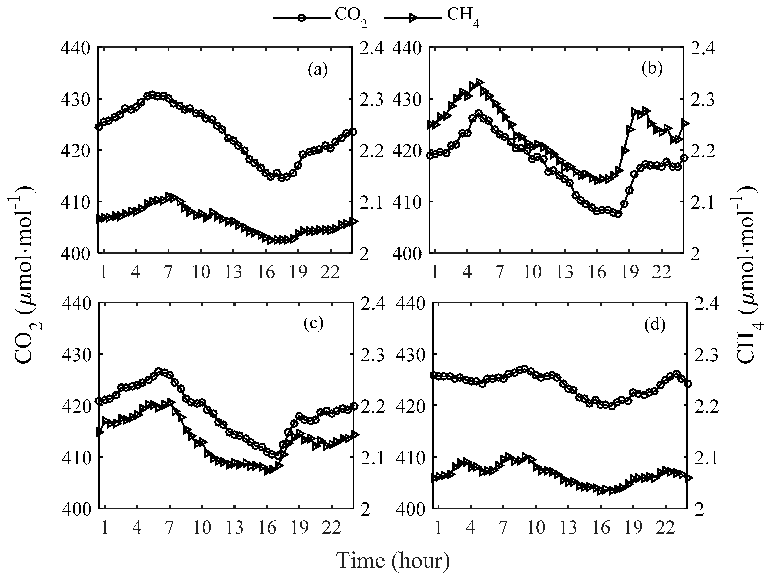
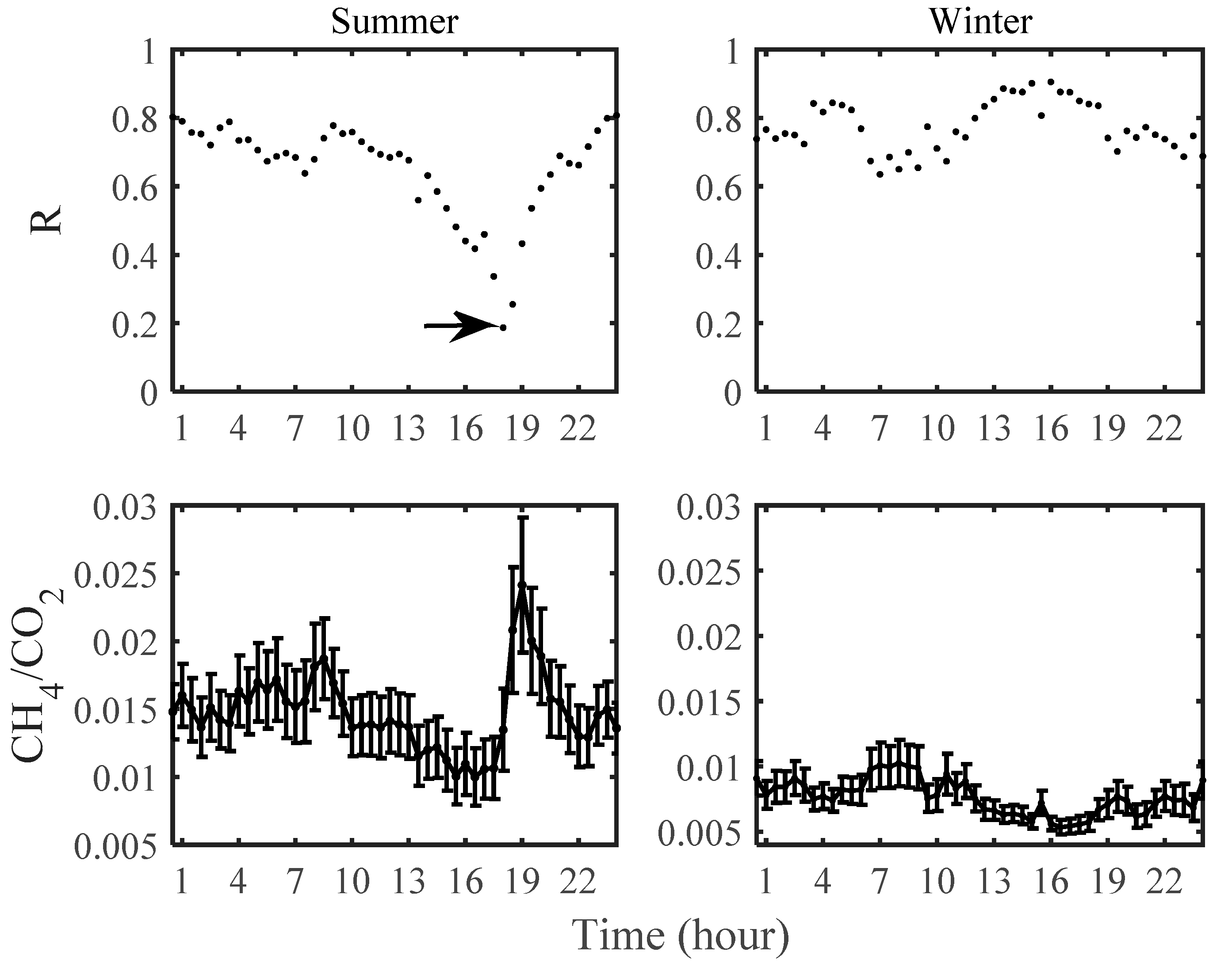
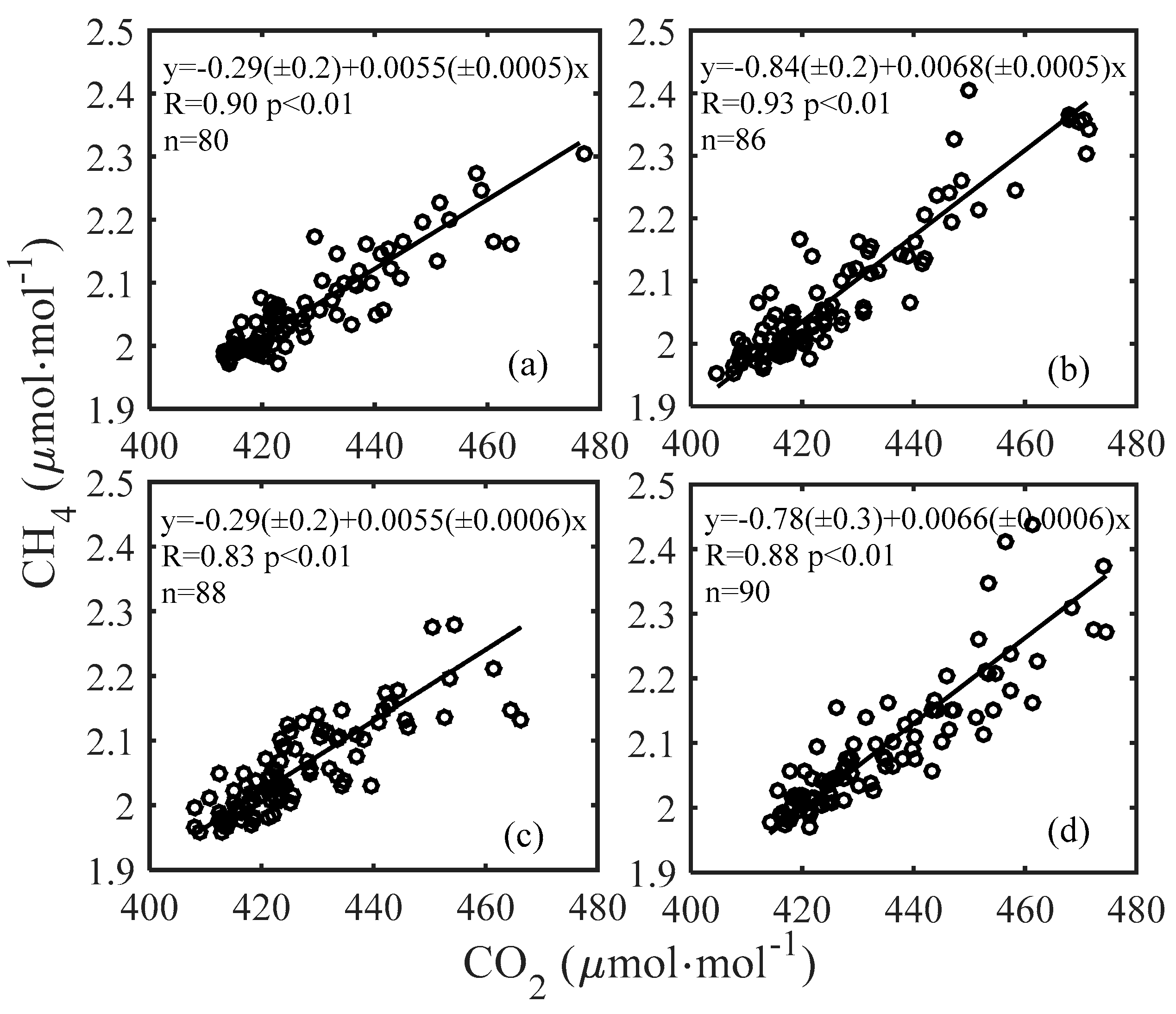
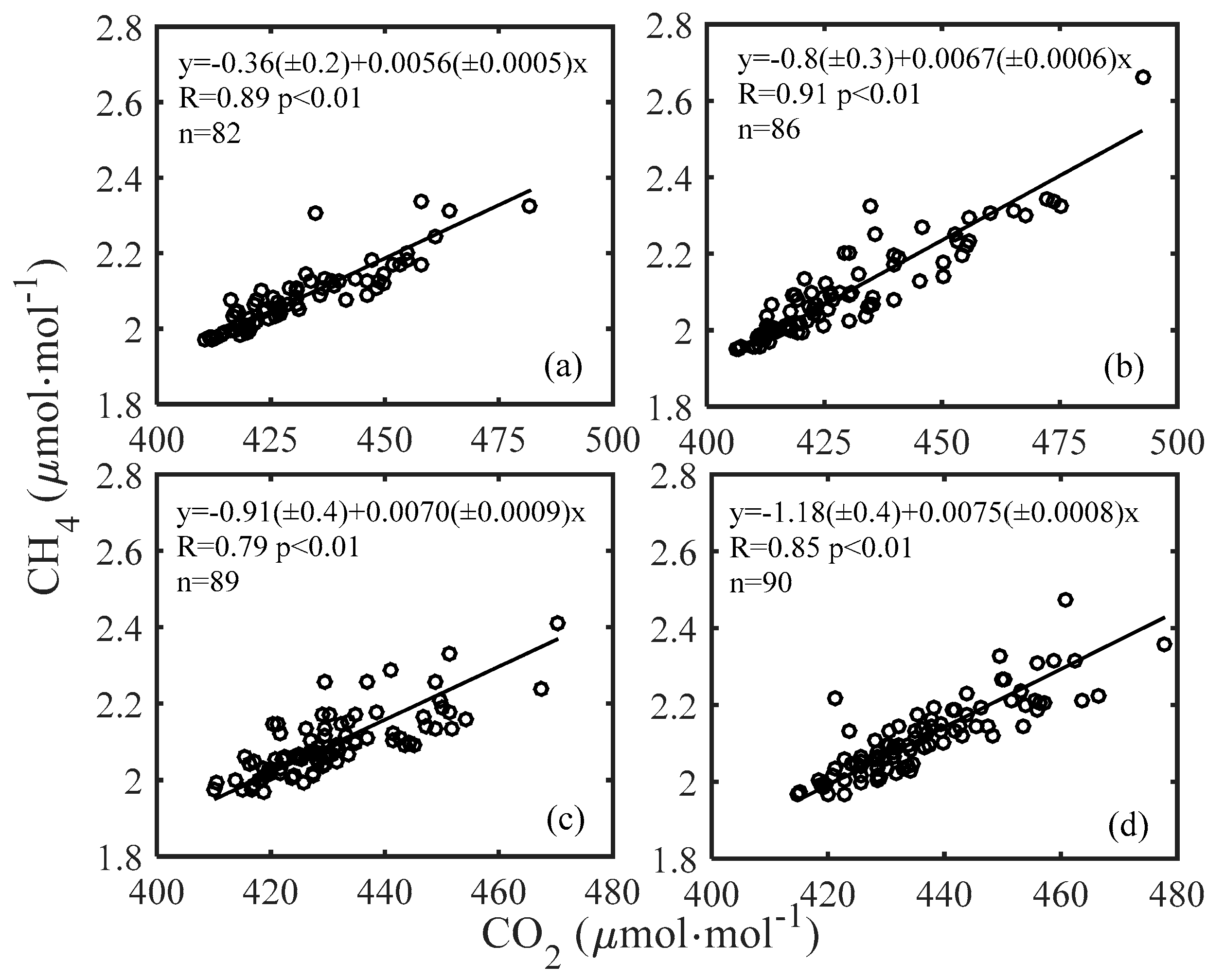
3.2. Diurnal and Inter-Annual Variations of the CH₄ Versus CO₂ Regression Slope

Figure 7 shows the diurnal variations of the CH₄ versus CO₂ regression slope and their linear correlation coefficients (R) for the summer and the winter in 2015. The slope value was determined for each half-hour period of the day, using all the data collected in the same half-hourly period. In the summer, the regression slope is marked by a sudden rise at around 18:00, coinciding with the onset of the surface inversion layer. The summertime R is high at night but has very low values in the afternoon. In the winter, the slope value is generally smaller than the summer value, and its diurnal variation is weak. The wintertime R fluctuates around 0.8. The fact that the regression slope is stable and that the R value is high in the winter is not a surprise. In the winter months, biological sources of CO₂ and CH₄ are much weaker than the anthropogenic sources. For this reason, the data in winter were selected for further study.

An important biological CH₄ source is wetland, including natural wetlands (offshore, coastal, swamp, lakes and rivers) and constructed wetlands. The total wetland area in the YRD is 5.4 × 10⁴ km² (2013 value) [36], or 15% of the total area of the YRD. However, wintertime wetland CH₄ flux is generally weak. A study found that the methane emission rate in a freshwater wetland in Australia is less than 0.01 mmol m⁻² h⁻¹ in the winter, which is much lower than that in the summer (1.3–3.3 mmol m⁻² h⁻¹) [69]. Similarly, CH₄ emissions from natural wetlands in the YRD are 1.98 × 10⁸ kg [51], far less than anthropogenic emissions in winter (3.10 × 10⁹ kg, Section 3.3). The Xixi wetland, one of the four major wetlands in the YRD, even becomes a weak sink of CH₄ in the winter (0.0019 mg m⁻² h⁻¹) [70]. Thus, CH₄ emissions from wetlands could be omitted when we compared the “top-down” and “bottom-up” estimates using wintertime observations.

Rice paddies are another important biological CH₄ source, contributing about 3.3–7.0% (18.3 × 10⁹ kg year⁻¹ to 8.8 × 10⁹ kg year⁻¹, 1901–2010) [71] of the global CH₄ emissions (5.58 × 10¹¹ kg year⁻¹, 2003–2012) [72]. China accounts for 20% of the rice production area in the world and the rice planting area in the YRD accounts for 18% of the China’s total [35,36,37,38]. The important conditions for CH₄ production are organic matter applied (such as rice straw) and anoxic soils established in flooded paddies. As a typical monsoon climate zone in southeastern China, the growth period for rice is from May to October [73]. During non-rice growing season in the winter, CH₄ emissions from non-permanently flooded rice paddies are about 4–6% of the emissions in the growth season [74], and were ignored in the comparison with our “top-down” estimation.

Figure 8 and Figure 9 are regression results using winter time observations made during 2012–2016. The regression was done separately for daytime (10:00–17:00 Beijing time) and nighttime (23:00–05:00 Beijing time) periods for consideration of different mixing conditions and source regions during the day and at night. In this regression, each data sample is a daytime or nighttime mean value. Taking the maximum drift over 24 h in CO₂ and CH₄ values (<120 ppb for CO₂ and <1 ppb for CH₄) for each point caused by the observational instrument into consideration, the slope was affected by <0.0001 ppm:ppm, which can be ignored comparing with the standard error caused by the fitting method (0.0005 in 2013). The daytime regression slope fluctuates between 0.0055 ± 0.0006 and 0.0068 ± 0.0005 ppm CH₄ per ppm CO₂ without an obvious interannual trend. The correlation coefficient R is greater than 0.8, and all four winters passed the 0.01 significance test.

The nighttime slope value increases from 0.0056 ± 0.0005 ppm/ppm for the winter of 2012–2013 to 0.0075 ± 0.0008 ppm/ppm for the winter of 2015–2016. With the exception of winter 2013–2014, the nighttime slope values are greater than the daytime values, implying more CH₄ emission per mole of CO₂ release by local anthropogenic sources than by regional sources. The correlation also passed the 0.01 significance test but the R values are slightly lower than the daytime R values.

An alternative approach to obtain the emissions ratio is to divide the CH₄ concentration enhancement over a background value by the CO₂ concentration enhancement. Here, we defined the clean background as the concentration at the 5th percentile. The emissions ratio, calculated as (CH_{4, mean}−CH_{4, 5%})/(CO_{2, mean}−CO_{2, 5%}) for the winter, is in good agreement with the slope of the CH₄ concentration versus CO₂ concentration (Figure S2).

In this study, we assumed that the daytime observations were influenced by sources located in the YRD. We used the EDGARv4.3.2 inventory data (2012) to understand the sensitivity of the emissions ratio to the spatial footprint. We found that by expanding the source region by 100 km from all sides of the YRD boundary, the CH₄:CO₂ emissions ratio changed by less than 1%.

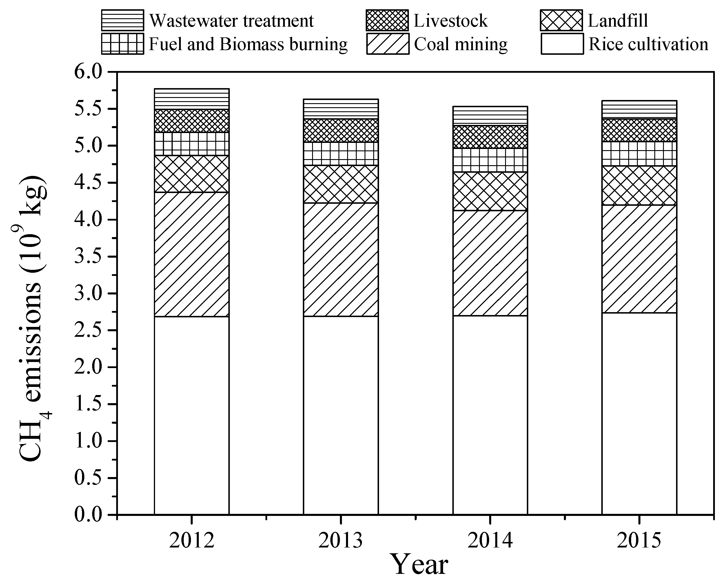
3.3. Inventory Results

Table 1. Anthropogenic CO₂ emissions in the YRD in 2012.

Sector	Emission (× 1011 kg)	Percent of Total (%)
Industrial energy consumption 1	13.03 (± 11%)	67.9
Industrial processes	4.40 (± 10%)	23.0
Transportation	1.35 (± 18%)	7.0
Household	0.40 (± 8%)	2.1
Total	19.18 (± 10%)	100

¹ CO₂ emissions in manufacturing, commerce, and construction are also included in this sector.

shows the results of the CO₂ emission in the YRD in 2012. Industrial energy consumption is the largest emitter, followed by industrial processes, and the residential sector is the smallest emitter. The emission estimate for the transportation sector has the largest relative uncertainty, mainly due to the lack of accurate data on the annual driving range and the emission factor for different vehicle types and driving conditions [75]. The total emission amount was 19.18 ×10¹¹ kg in 2012. The Monte Carlo method gives an overall uncertainty of 10%. For comparison the total emission amount in 2009 was 15.35 × 10¹¹ kg [51].

The annual CO₂ emission for 2012–2015 is shown in Figure 10. The growth rate was 3% from 2012 to 2013 and decreased to 0.5% from 2014 to 2015. The reduced growth was mainly caused by the decrease in the industrial energy emission.

Similarly,

Table 2. Anthropogenic CH₄ emissions in the Yangtze River Delta in 2012, based on the IPCC inventory method.

Sector	Emission (× 109 kg)	Percent of Total (%)
Rice cultivation	2.68 (± 12%)	46.3
Landfill	0.50 (± 35%)	8.7
Wastewater treatment	0.28 (± 40%)	4.8
Livestock	0.31 (± 14%)	5.4
Fuel and Biomass burning	0.32 (± 17%)	5.6
Coal mining	1.69 (± 30%)	29.2
Total	5.78 (± 21%)	100

shows the anthropogenic CH₄ emissions in the YRD in 2012. Rice cultivation and coal mining are the major sources of anthropogenic CH₄ emissions. Emission estimates for landfills, wastewater treatment and fuel burning (traffic) emissions have large uncertainties. The total regional emission was 5.78 × 10⁹ kg in 2012, increasing by 9.7% compared to that reported for 2009 [51]. The uncertainty of the total estimate (21%) is much greater than the uncertainty (10%) of the CO₂ emission estimate (Table 1), supporting the use of CO₂ as a tracer gas to calculate the CH₄ emission with the atmospheric method.

Figure 11 shows the annual anthropogenic CH₄ emission in the YRD from 2012 to 2015. There was a slight downward trend during the study period, but there was a slight increase from 2014 to 2015.

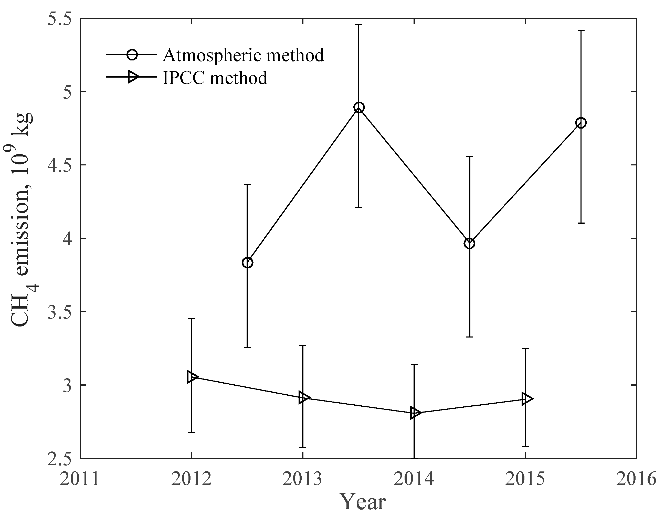
3.4. Comparison of CH₄ Emission Estimates between the Methods

Figure 12 shows the comparison of the annual anthropogenic CH₄ emissions obtained with the two methods. In this comparison, emissions from rice cultivation were excluded from the IPCC estimate because no rice is grown in the winter months. The “top-down” atmospheric estimate fluctuates year by year, in the range from 3.84 × 10⁹ kg to 4.89 × 10⁹ kg, which is 1.2–1.7 times the IPCC result.

4. Discussion

4.1. Annual Growth Rates of CH₄ and CO₂ Concentrations

The observation lasted nearly five years. Due to the lack of data in some months, the annual average is not representative, thus the linear increase rate of monthly averages was used to characterize the annual growth rate. The CO₂ growth rate at the MLW site from 2012 to 2017 was 2.5 ± 0.7 ppm year⁻¹, which is 9% higher than observed at the WLG background station (2.3 ± 0.2 ppm year⁻¹). A similar result was obtained from observations near Beijing, showing a 24% higher growth rate than at WLG [76]. The large growth rate is consistent with the anthropogenic CO₂ emissions trend in the YRD with an increase of 30% from 15.35 × 10¹¹ kg in 2009 [51] to 19.95 × 10¹¹ kg in 2015 (Figure 10). In this period, emissions from the transport sector increased by 88%, in line with the increasing car ownership, while emissions from industrial processes were nearly unchanged [51].

The annual growth rate of CH₄ at MLW (9.5 ± 4.7 ppb year⁻¹) is nearly twice that at WLG (6.2 ± 1.7 ppb year⁻¹). The increasing trend at MLW is close to that in the Lin’an station in Zhejiang Province, which is also located in the center of YRD, with a growth rate of 8.0 ± 1.2 ppb year⁻¹ from 2009 to 2011 [77]. The growth rate at WLG from 2012 to 2016 was quite similar to global mean growth rate (about 6 ppb year⁻¹, 2010–2014) [78,79]. The annual trend of CH₄ is 4.8 ppb year⁻¹ (2008–2013) at the Zhongshan station in Antarctica, which is the least influenced by human activities [80,81]. At the Shangdianzi regional background station in Beijing, atmospheric CH₄ concentration influenced by airmasses passing through the highly developed Beijing Municipality, Tianjin Municipality and Hebei Province increased at a rate of 10 ± 0.1 ppb year⁻¹ from 2009 to 2013, whereas atmospheric CH₄ concentrations influenced by airmasses originating from Russia, Mongolia, and the Inner Mongolia Autonomous Region of China increased at a rate of 6 ± 0.1 ppb year⁻¹ over the same period [82].

One reason for the high CH₄ growth rate at the MLW site is the steady increase in anthropogenic emissions according to the inventory data, although the “top-down” estimate does not reveal such a trend in anthropogenic emissions. Another reason may be related to the expansion of wetland areas. According to two national surveys of wetland resources, the total wetland area in the YRD obtained by the second census (2009–2013) increased by 54% in comparison with the first (1995–2003), from 3.5 × 10⁴ km² to 5.4 × 10⁴ km² [36]. About 67% of this growth is contributed by constructed wetlands, which increased by nearly 700%. In natural wetlands around the world, the CH₄ emission flux, ranging from 7.0 × 10³ to 2.8 × 10⁴ kg km⁻² year⁻¹ with an average of 2.1 × 10⁴ kg km⁻² year⁻¹ [83,84] is lower than in constructed wetlands (ranging from 1.3 × 10³ to 1.5 × 10⁵ kg km⁻² year⁻¹, with an average of 4.7 × 10⁴ kg km⁻² year⁻¹) [85]. The annual total emissions by wetlands for the two time periods (1995–2003 and 2009–2013) aere 1.89 × 10⁸ kg year⁻¹ (range 1.6 × 10⁸ to 14.8 × 10⁸ kg year⁻¹) and 2.98 × 10⁸ kg year⁻¹ (range 2.5 × 10⁸ to 23.3 × 10⁸ kg year⁻¹), respectively, using the Tier 1 approach provided by 2006 IPCC guidelines for moist and warm climates [8]. This method only considers diffusive emissions for natural wetlands during ice-free periods. Emissions from wetlands in two national surveys were 6.1% and 9.6% anthropogenic emission (excluding rice cultivation) in 2012 (3.1 (± 0.5) × 10⁹ kg, Table 2).

4.2. Comparison of the CH₄/CO₂ Emissions Ratio

Some sources, such as transportation and landfills, release both CH₄ and CO₂, but their CH₄/CO₂ emissions ratios are very different. The average CH₄/CO₂ emissions ratio of vehicle traffic is 4.6 (± 0.2) × 10⁻⁵ ppm/ppm according to observations in traffic tunnels in Switzerland [86], indicating that CH₄ emissions from traffic emissions account for only a small fraction of the anthropogenic emission. In a study of eight cities in China, the traffic emissions ratio is 7.0 (± 3.6) × 10⁻³ ppm/ppm [87]. The ratio is much larger than that in Switzerland. In comparison, CH₄ comprises up to 61% (median: 34%) of the total volume of landfill gas, with the remaining 3% to 69% (median: 33%) being CO₂ [88,89]. In the case of wetlands, the emissions ratio varies with the type of wetlands and sometimes is negative because they act as sources of CH₄ but sinks of CO₂ [90,91,92]. The emissions ratio estimated from the regression slope is a composite signal of all the sources at the regional scale.

Table S1 summarizes the CH₄/CO₂ emissions ratio observed in different parts of the world. All these values were obtained as the regression slope of atmospheric CH₄ concentration against the CO₂ concentration. Some of these slope values were given by the cited literature, while others were estimated from the original concentration data. Our emissions ratio is close to those observed in Los Angeles and Pasadena, USA, but is higher than that observed in the daytime in Nanjing, China. The highest values occur in northern latitude remote sites far away from major industrial activities, such as Barrow, USA and Alert, Canada, due to abundant wetlands at these latitudes (>50% land area) [93]. About 60% of the total CH₄ emission from natural wetlands come from those between latitude 50° N to 70° N [83].

4.3. Comparison between the IPCC Method and the Atmospheric Method

Shen et al. measured atmospheric CO₂ and CH₄ molar fraction at a suburban site in Nanjing from June 2010 to April 2011 [51]. They argued that the regression slope from daytime data represents emissions ratio of sources in the YRD, and the regression slope from nighttime data represents emissions ratio of the local sources in the Nanjing Municipality. Their atmospheric estimate for CH₄ emission for sources in Nanjing is 200% higher than the IPCC estimate [51]. If we assume that the nighttime data in this study are also indicative of local sources in the Wuxi Municipality, our atmospheric estimate of the CH₄ emission in the winter would be 1.8 × 10⁸–2.3 ×10⁸ kg, which is 4.4–5.7 times as large as the value calculated with the IPCC method (after exclusion of rice paddy emissions;

Table 3. Anthropogenic CH₄ emissions in Wuxi in 2012 based on the IPCC inventory method.

Sector	Emission (× 107 kg)	Percent of Total (%)
Rice cultivation	3.05 (± 13%)	42.8
Landfill	1.81 (± 38%)	25.4
Wastewater treatment	1.45 (± 40%)	20.3
Livestock	0.48 (± 22%)	6.7
Fuel and Biomass burning	0.34 (± 21%)	4.8
Coal mining	—	—
Total	7.13 (± 26%)	100

). The IPCC method is far more uncertain at the urban scale than at the regional scale, for several reasons. First, cities do not have clear boundaries and direct emissions calculated based on urban statistics ignore some emissions of cities, such as aviation and waterways, so the total emission will be underestimated [94]. As the spatial scale increases, the dependence of the accounting area on cross-boundary transport of energy and material is smaller, and errors due to indirect emissions are reduced [95]. Second, emission factors at the cities are not measured accurately. Third, wastewater treatment and landfill are the two largest source categories in Wuxi, accounting for 45.6% of the city’s total CH₄ emissions; these two sources have the largest uncertainty.

In comparison with the IPCC estimate for the YRD in the winter, the “top-down” atmospheric estimate in this study is 1.2–1.7 times the IPCC result. Shen et al.’s estimate of CH₄ emission from the atmospheric method is 20% lower [51] than the IPCC estimate, even though their measurement and our measurement both took place in the same region (YRD) and not too far from each other (170 km apart). One possible reason for the difference is that Shen et al.’s observation site is not far away from industrial complexes and traffic roads. Traffic CH₄/CO₂ emissions ratio is generally much lower than regional emissions ratios, as noted above. According to the “bottom-up” results provided by the Emissions Database for Global Atmospheric Research (EDGAR), the global CH₄/CO₂ emissions ratios in the chemical production sector, the metal production sector, and the public electricity and heat production sector were 1.2 × 10⁻³, 6.4 × 10⁻⁴ and 7.6 × 10⁻⁵ ppm/ppm, respectively in 2012 (http://edgar.jrc.ec.europa.eu/overview.php?v=432&SECURE=123) [96]. The situation is a little different in China. The CH₄/CO₂ emissions ratio is bigger for the chemical production sector (1.8 × 10⁻³ ppm/ppm), and is smaller for the metal production sector (4.7 × 10⁻⁴ ppm/ppm) and the public electricity and heat production sector (3.4 × 10⁻⁵ ppb/ppm). Thus, the CH₄/CO₂ emissions ratio for industrial complexes should be lower than regional emissions ratios. Because our measurement was made at a rural system not directly impacted by local traffic and industrial emissions (Figure S1), our emissions ratio should be more representative than that reported in [51].

Another reason for the difference between our study and the study by Shen et al. [51] is different source areas between Nanjing and MLW. Hu et al. [97] simulated the atmospheric CO₂ concentration in Nanjing City using the WRF-STILT model. They found that the NUIST site is mainly affected by the central and eastern regions of Anhui Province and the central and western regions of Jiangsu Province, with greater concentration contribution weights than other regions in the YRD.

Previous studies have also reported that estimates of CH₄ emission based on the “top-down” atmospheric method are higher than the “bottom-up” inventory estimates. In the Los Angeles metropolitan area in California, USA, anthropogenic CH₄ emissions calculated from two “top-down” approaches are 1.3–1.8 and 1.2–1.6 times, respectively, of the “bottom-up” estimates [20,98]. The US EPA inventory and EDGAR, two “bottom-up” methods, are shown to underestimate CH₄ emissions in the United States by a factor of about 1.5 and 1.7, with the underestimation coming from two sectors: livestock and fossil fuel extraction and processing [99]. That “bottom-up” results are generally smaller indicate that there are unknown emission sources or underestimates of the emission capacity of known sources, such as landfills, coal mining and wastewater treatment. Some scholars have found that based on carbon isotope observations, CH₄ emissions from landfills and ruminants are underestimated by the IPCC method [100]. In China, the methane emission rate is reported to be eight times the IPCC emission estimate for natural gas vehicles [78]. If this result is taken into consideration, the anthropogenic CH₄ emissions in the YRD would increase by 2.4% in 2015. In the urban Boston area, USA, natural gas loss rate from transmission, distribution and end use was 2.7 ± 0.6% of the total delivered gas, which is more than twice the result of the emission inventory [101]. In 2016, the length of natural gas pipeline reached 5.51 × 10⁵ km in China, although the CH₄ concentration measurements along urban street transects in eight Chinese cities show no evidence of pipeline leakage [87].

5. Conclusions

Continuous observation of atmospheric CO₂ and CH₄ mole fraction was made at the MLW station near Wuxi at Lake Taihu from May 2012 to April 2017. These measurements were combined with anthropogenic CO₂ emission data in a “top-down” method to obtain an estimate of the anthropogenic CH₄ emission in the YRD. For comparison, the CH₄ emission was also calculated with the IPCC inventory method. The key results are as follows:

(1) The growth rates of the CO₂ and CH₄ molar fractions at the MLW site were 2.5 ± 0.7 ppm year⁻¹ and 9.5 ± 4.7 ppb year⁻¹, respectively, which are 9% and 53% higher than that observed at WLG over the same period.

(2) To avoid the interference of biological sources, we used the wintertime CO₂ and CH₄ concentration data to obtain the CH₄/CO₂ emissions ratio. Results indicate that the emissions ratio fluctuates between 0.0055 ± 0.0006 ppm/ppm (winters of 2012–2013 and 2014–2015) and 0.0068 ± 0.0005 ppm/ppm (winter of 2013–2014). These ratios are similar to those observed in Los Angeles and Pasadena, USA.

(3) According to the “top-down” method, the annual average anthropogenic emission of CH₄ in the YRD from 2012 to 2015 is 4.37 (± 0.61) × 10⁹ kg year⁻¹ (excluding rice cultivation), which is 1.2–1.7 times the result from the IPCC inventory.

(4) The “top-down” method also suggests that at the local scale, the IPCC inventory estimate for anthropogenic CH₄ emission in the Wuxi municipality may be biased low by 4.4−5.7 times.

References

1. World Meteorological Organization (WMO). Greenhouse Gas Bulletin: The State of Greenhouse Gases in the Atmosphere Based on Global Observations through 2017; WMO: Geneva, Switzerland, 2018. [Google Scholar]
2. IPCC. The IPCC Fifth Assessment Report—Climate Change 2013: The Physical Science Basis; Working Group I, IPCC Secretariat: Geneva, Switzerland, 2013. [Google Scholar]
3. Solomon, S.; Intergovernmental Panel on Climate Change. Working Group I, Climate Change 2007: The Physical Science Basis: Contribution of Working Group I to the Fourth Assessment Report of the Intergovernmental Panel on Climate Change; Cambridge University Press: Cambridge, UK; New York, NY, USA, 2007. [Google Scholar]
4. Dlugokencky, E.J. NOAA/ESRL. Available online: www.esrl.noaa.gov/gmd/ccgg/trends_ch4/ (accessed on 24 March 2019).
5. Dlugokencky, E.J.; Bruhwiler, L.; White, J.W.C.; Emmons, L.K.; Novelli, P.C.; Montzka, S.A.; Masarie, K.A.; Lang, P.; Crotwell, A.M.; Miller, J.B.; et al. Observational constraints on recent increases in the atmospheric CH4 burden. Geophys. Res. Lett. 2009, 36, 252–260. [Google Scholar] [CrossRef]
6. Forster, P.; Ramaswamy, V.; Artaxo, P.; Bernsten, T.; Betts, R.; Fahey, D.W.; Haywood, J.; Lean, J.; Lowe, D.C.; Myhre, G.; et al. Changes in Atmospheric Constituents and in Radiative Forcing. Chapter 2. Climate Change 2007: The Physical Science Basis; Cambridge University Press: Cambridge, UK, 2007; pp. 129–234. [Google Scholar]
7. Aydin, M.; Verhulst, K.R.; Saltzman, E.S.; Battle, M.O.; Montzka, S.A.; Blake, D.R.; Tang, Q.; Prather, M.J. Recent decreases in fossil-fuel emissions of ethane and methane derived from firn air. Nature 2011, 476, 198–201. [Google Scholar] [CrossRef] [PubMed] [Green Version]
8. IPCC. 2006 IPCC Guidelines for National Greenhouse Gas Inventories, Prepared by the National Greenhouse Gas Inventories Programme; Eggleston, HS., Buendia, L., Miwa, K., Ngara, T., Tanabe, K., Eds.; IGES: Kanagawa, Japan, 2006. [Google Scholar]
9. Yue, Q.; Zhang, G. Preliminary estimation of methane emission and its distribution in China. Geogr. Res. 2012, 31, 1561–1570. (In Chinese) [Google Scholar] [CrossRef]
10. Boon, A.; Broquet, G.; Clifford, D.J.; Chevallier, F.; Butterfield, D.M.; Pison, I.; Ramonet, M.; Paris, J.D.; Ciais, P. Analysis of the potential of near ground measurements of CO2 and CH4 in London, UK for the monitoring of city-scale emissions using an atmospheric transport model. Atmos. Chem. Phys. 2016, 16, 6735–6756. [Google Scholar] [CrossRef]
11. Chen, C.; Liu, C.; Li, Z.; Wang, H.; Zhang, Y.; Wang, L. Uncertainty analysis for evaluating methane emissions from municipal solid waste landfill in Beijing. Environ. Sci. 2012, 33, 208–215. (In Chinese) [Google Scholar]
12. Pei, Z.; Ou Yang, H.; Zhou, C. A study on carbon fluxes from alpine grassland ecosystem on Tibetan Plateau. Acta Ecol. Sin. 2003, 23, 231–236. (In Chinese) [Google Scholar] [CrossRef]
13. Minamikawa, K.; Yagi, K.; Tokida, T.; Sander, B.O.; Wassmann, R. Appropriate frequency and time of day to measure methane emissions from an irrigated rice paddy in Japan using the manual closed chamber method. Greenh. Gas Meas. Manag. 2012, 2, 118–128. [Google Scholar] [CrossRef]
14. Winton, R.S.; Richardson, C.J. A cost-effective method for reducing soil disturbance-induced errors in static chamber measurement of wetland methane emissions. Wetl. Ecol. Manag. 2016, 24, 419–425. [Google Scholar] [CrossRef]
15. Lee, X. Fundamentals of Boundary-Layer Meteorology; Springer International Publishing: Cham, Switzerland, 2018. [Google Scholar]
16. Conway, T.J.; Steele, L.P. Carbon dioxide and methane in the Arctic atmosphere. J. Atmos. Chem. 1989, 9, 81–99. [Google Scholar] [CrossRef]
17. Conway, T.J.; Steele, L.P.; Novelli, P.C. Correlations among atmospheric CO2, CH4, and CO in the Arctic, March 1989. Atmos. Environ. Part A Gen. Top. 1993, 27, 2881–2894. [Google Scholar] [CrossRef]
18. Hansen, A.D.A.; Conway, T.J.; Strele, L.P.; Bodhaine, B.A.; Thoning, K.W.; Tans, P.; Novakov, T. Correlations among combustion effluent species at Barrow, Alaska: Aerosol black carbon, carbon dioxide, and methane. J. Atmos. Chem. 1989, 9, 283–299. [Google Scholar] [CrossRef]
19. Wunch, D.; Wennberg, P.O.; Toon, G.C.; Keppel-Aleks, G.; Yavin, Y.G. Emissions of greenhouse gases from a North American megacity. Geophys. Res. Lett. 2009, 36, 139–156. [Google Scholar] [CrossRef]
20. Wong, K.W.; Fu, D.; Pongetti, T.J.; Newman, S.; Kort, E.A.; Duren, R.; Hsu, Y.K.; Miller, C.E.; Yung, Y.L.; Sander, S.P. Mapping CH4: CO2 ratios in Los Angeles with CLARS-FTS from Mount Wilson, California. Atmos. Chem. Phys. 2015, 15, 241–252. [Google Scholar] [CrossRef]
21. Lelieveld, J.; Crutzen, P.J.; Dentener, F.J. Changing concentration, lifetime and climate forcing of atmospheric methane. Tellus Ser. B Chem. Phys. Meteorol. 1998, 50, 128–150. [Google Scholar] [CrossRef]
22. Zhao, Y.; Nielsen, C.P.; Mcelroy, M.B. China’s CO2 emissions estimated from the bottom up: Recent trends, spatial distributions, and quantification of uncertainties. Atmos. Environ. 2012, 59, 214–223. [Google Scholar] [CrossRef]
23. Lee, X.; Bullock, O.R.; Andres, R.J. Anthropogenic emission of mercury to the atmosphere in the northeast United States. Geophys. Res. Lett. 2001, 28, 1231–1234. [Google Scholar] [CrossRef] [Green Version]
24. Wang, Y.; Munger, J.W.; Xu, S.; McElroy, M.B.; Hao, J.; Nielsen, C.P.; Ma, H. CO2 and its correlation with CO at a rural site near Beijing: Implications for combustion efficiency in China. Atmos. Chem. Phys. 2010, 10, 8881–8897. [Google Scholar] [CrossRef]
25. Suntharalingam, P.; Jacob, D.J.; Palmer, P.I.; Logan, J.A.; Yantosca, R.M.; Xiao, Y.; Evans, M.J. Improved quantification of Chinese carbon fluxes using CO2/CO correlations in Asian outflow. J. Geophys. Res. 2004, 109, 159–172. [Google Scholar] [CrossRef]
26. Zhu, T.; Yang, G.; Su, W.; Wan, R. Coordination evaluation between urban land intensive use and economic society development in the Yangtze River Delta. Resour. Sci. 2009, 31, 1109–1116. (in Chinese). [Google Scholar]
27. Lee, X.; Liu, S.; Xiao, W.; Wang, W.; Gao, Z.; Cao, C.; Hu, C.; Hu, Z.; Shen, S.; Wang, Y.; et al. The Taihu eddy flux network: an observational program on energy, water, and greenhouse gas fluxes of a large freshwater lake. Bull. Am. Meteorol. Soc. 2014, 95, 1583–1594. [Google Scholar] [CrossRef]
28. Xiao, W.; Liu, S.; Li, H.; Xiao, Q.; Wang, W.; Hu, Z.; Hu, C.; Gao, Y.; Shen, J.; Zhao, X.; et al. A flux-gradient system for simultaneous measurement of the CH4, CO2, and H2O fluxes at a lake-air interface. Environ. Sci. Technol. 2014, 48, 14490–14498. [Google Scholar] [CrossRef] [PubMed]
29. Flores, E.; Viallon, J.; Choteau, T.; Moussay, P.; Wielgosz, R.I.; Kang, N.; Kim, B.M.; Zalewska, E.; van der Veen, A.M.H.; Konopelko, L.; et al. International comparison CCQM-K82: Methane in air at ambient level (1800 to 2200) nmol/mol. Metrologia 2015, 52, 1–129. [Google Scholar] [CrossRef]
30. Flores, E.; Viallon, J.; Choteau, T.; Moussay, P.; Idrees, F.; Wielgosz, R.I.; Lee, J.; Zalewska, E.; Nieuwenkamp, G.; van der Veen, A.; et al. CCQM-K120 (Carbon dioxide at background and urban level). Metrologia 2019, 56, 1–178. [Google Scholar] [CrossRef]
31. State Statistical Bureau. China Energy Statistical Yearbook 2012; China Statistical Press: Beijing, China, 2013. (In Chinese)
32. State Statistical Bureau. China Energy Statistical Yearbook 2013; China Statistical Press: Beijing, China, 2014. (In Chinese)
33. State Statistical Bureau. China Energy Statistical Yearbook 2014; China Statistical Press: Beijing, China, 2015. (In Chinese)
34. State Statistical Bureau. China Energy Statistical Yearbook 2015; China Statistical Press: Beijing, China, 2016. (In Chinese)
35. State Statistical Bureau. China Statistical Yearbook 2012; China Statistical Press: Beijing, China, 2013. (In Chinese)
36. State Statistical Bureau. China Statistical Yearbook 2013; China Statistical Press: Beijing, China, 2014. (In Chinese)
37. State Statistical Bureau. China Statistical Yearbook 2014; China Statistical Press: Beijing, China, 2015. (In Chinese)
38. State Statistical Bureau. China Statistical Yearbook 2015; China Statistical Press: Beijing, China, 2016. (In Chinese)
39. State Statistical Bureau. China Rural Statistical Yearbook 2012; China Statistical Press: Beijing, China, 2013. (In Chinese)
40. State Statistical Bureau. China Rural Statistical Yearbook 2013; China Statistical Press: Beijing, China, 2014. (In Chinese)
41. State Statistical Bureau. China Rural Statistical Yearbook 2014; China Statistical Press: Beijing, China, 2015. (In Chinese)
42. State Statistical Bureau. China Rural Statistical Yearbook 2015; China Statistical Press: Beijing, China, 2016. (In Chinese)
43. Cao, G.; Zhang, X.; Zhen, F.; Wang, Y. Estimating the quantity of crop residues burnt in open field in China. Resour. Sci. 2006, 28, 9–13. (in Chinese). [Google Scholar] [CrossRef]
44. Qiu, L.; Yang, G.; Bi, Y. Discussion on the conditions and countermeasures of developing marsh gas in rural areas of west China. Agric. Res. Arid Areas 2005, 23, 200–204. (In Chinese) [Google Scholar] [CrossRef]
45. Scheutz, C.; Kjeldsen, P.; Bogner, J.E.; Visscher, A.D.; Gebert, J.; Hilger, H.A.; Huber-Humer, M.; Spokas, K. Microbial methane oxidation processes and technologies for mitigation of landfill gas emissions. Waste Manag. Res. 2009, 27, 409–455. [Google Scholar] [CrossRef] [PubMed]
46. Cai, B. Analysis of the features of methane emissions from landfills of China in 2012. Environ. Eng. 2016, 34, 1–4. (In Chinese) [Google Scholar] [CrossRef]
47. Chen, D.; Wang, M.; Shang Guan, X.; Huang, J.; Rasmussen, R.A.; Khalil, M.A.K. Methane emission from rice fields in the south-east China. Adv. Earth Sci. 1993, 8, 47–54. (in Chinese). [Google Scholar]
48. Wang, M. Methane emission and mechanisms of methane production, oxidation, transportation in the rice fields. Chin. J. Atmos. Sci. 1998, 22, 600–612. (In Chinese) [Google Scholar] [CrossRef]
49. Min, J.; Hu, H. Calculation of greenhouse gases emission from agricultural production in China. China Popul. Resour. Environ. 2012, 22, 21–27. (In Chinese) [Google Scholar] [CrossRef]
50. Zhao, B. The Research on the Surface Mine Group Development & Design Theory and Engineering Optimization; China University of Mining & Technology: Beijing, China, 2015. (In Chinese) [Google Scholar]
51. Shen, S.; Dong, Y.; Wei, X.; Liu, S.; Lee, X. Constraining anthropogenic CH4 emissions in Nanjing and the Yangtze River Delta, China, using atmospheric CO2 and CH4 mixing ratios. Adv. Atmos. Sci. 2014, 31, 1343–1352. [Google Scholar] [CrossRef]
52. Yang, D.; Shen, S.; Zhang, M.; Lee, X.; Xiao, W. Uncertainty analysis on the estimation of CO2 and CH4 emission inventory over Nanjing and Yangtze River Delta. J. Meteorol. Sci. 2014, 34, 325–334. (In Chinese) [Google Scholar] [CrossRef]
53. Ramírez, A.; Keizer, C.D.; Sluijs, J.P.V.D.; Olivier, J.; Brandes, L. Monte Carlo analysis of uncertaintes in the Netherlands greenhouse gas emission inventory for 1990–2004. Atmos. Environ. 2008, 42, 8263–8272. [Google Scholar] [CrossRef]
54. Rypdal, K.; Winiwarter, W. Uncertainties in greenhouse gas emission inventories evaluation, comparability and implications. Environ. Sci. Policy 2001, 4, 107–116. [Google Scholar] [CrossRef]
55. Amstel, A.R.V.; Olivier, J.G.J.; Ruyssenaars, P.G. Monitoring of greenhouse gases in the Netherlands: Uncertainty and priorities for improvement. In Proceedings of the National Workshop, Bilthoven, The Netherlands, 1 September 1999. [Google Scholar]
56. Winiwarter, W.; Rypdal, K. Assessing the uncertainty associated with national greenhouse gas emission inventories: A case study for Austria. Atmos. Environ. 2001, 35, 5425–5440. [Google Scholar] [CrossRef]
57. Wehr, R.; Saleska, S.R. The long-solved problem of the best-fit straight line: Application to isotopic mixing lines. Biogeosciences 2016, 14, 17–29. [Google Scholar] [CrossRef]
58. Rotty, R.M. Estimates of seasonal variation in fossil fuel CO2 emissions. Tellus 1987, 39, 184–202. [Google Scholar] [CrossRef]
59. Li, Y.; Deng, J.; Mu, C.; Xing, Z.; Du, K. Vertical distribution of CO2, in the atmospheric boundary layer: Characteristics and impact of meteorological variables. Atmos. Environ. 2014, 91, 110–117. [Google Scholar] [CrossRef]
60. Winderlich, J.; Gerbig, C.; Kolle, O.; Heimann, M. Inferences from CO2 and CH4 concentration profiles at the Zotino Tall Tower Observatory (ZOTTO) on regional summertime ecosystem fluxes. Biogeosciences 2014, 10, 15337–15372. [Google Scholar] [CrossRef]
61. Wang, Y. MeteoInfo: GIS software for meteorological data visualization and analysis. Meteorol. Appl. 2014, 21, 360–368. [Google Scholar] [CrossRef]
62. Wang, Y.; Zhang, X.; Draxler, R.R. TrajStat: GIS-based software that uses various trajectory statistical analysis methods to identify potential sources from long-term air pollution measurement data. Environ. Model. Softw. 2009, 24, 938–939. [Google Scholar] [CrossRef]
63. Sigler, J.M.; Lee, X. Recent trends in anthropogenic mercury emission in the northeast United States. J. Geophys. Res. Atmos. 2006, 111, 3131–3148. [Google Scholar] [CrossRef]
64. Zhang, F.; Fukuyama, Y.; Wang, Y.; Fang, S.; Li, P.; Fan, T.; Zhou, L.; Liu, X.; Meinhardt, F.; Emiliani, P. Detection and attribution of regional CO2 concentration anomalies using surface observations. Atmos. Environ. 2015, 123, 88–101. [Google Scholar] [CrossRef]
65. Obrist, D.; Conen, F.; Vogt, R.; Siegwolf, R.; Alewell, C. Estimation of Hg0 exchange between ecosystems and the atmosphere using 222Rn and Hg0 concentration changes in the stable nocturnal boundary layer. Atmos. Environ. 2006, 40, 856–866. [Google Scholar] [CrossRef]
66. Zhou, L.; Tang, J.; Wen, Y.; Li, J.; Yan, P.; Zhang, X. The impact of local winds and long-range transport on the continuous carbon dioxide record at Mount Waliguan, China. Tellus B 2003, 55, 145–158. [Google Scholar] [CrossRef]
67. Zhang, F.; Zhou, L.; Xu, L. Temporal variation of atmospheric CH4 and the potential source regions at Waliguan, China. Sci. China Earth Sci. 2013, 56, 727–736. (In Chinese) [Google Scholar] [CrossRef]
68. Xu, J.; Lee, X.; Xiao, W.; Cao, C.; Liu, S.; Wen, X.; Xu, J.; Zhang, Z.; Zhao, J. Interpreting the 13C/12C ratio of carbon dioxide in an urban airshed in the Yangtze River Delta, China. Atmos. Chem. Phys. 2017, 17, 3385–3399. [Google Scholar] [CrossRef]
69. Boon, P.I.; Mitchell, A. Methanogenesis in the sediments of an Australian freshwater wetland, Comparison with aerobic decay, and factors controlling methanogenesis. Fems. Microbiol. Ecol. 1995, 18, 175–190. [Google Scholar] [CrossRef]
70. Qin, S.; Tang, J.; Pu, J.; Xu, Y.; Dong, P.; Jiao, L.; Guo, J. Fluxes and influencing factors of CO2 and CH4 in Hangzhou Xixi wetland, China. Earth Environ. 2016, 44, 513–519. (In Chinese) [Google Scholar] [CrossRef]
71. Zhang, B.; Tian, H.; Ren, W.; Tao, B.; Lu, C. Methane emissions from global rice fields: Magnitude, spatiotemporal patterns, and environmental controls. Glob. Biogeochem. Cycle 2016, 30, 1246–1263. [Google Scholar] [CrossRef]
72. Saunois, M.; Bousquet, P.; Poulter, B.; Peregon, A.; Ciais, P.; Canadell, J.G.; Dlugokencky, E.J.; Etiope, G.; Bastviken, D.; Houweling, S.; et al. The global methane budget 2000–2012. Earth Syst. Sci. Data 2016, 8, 697–751. [Google Scholar] [CrossRef] [Green Version]
73. Wang, X.; Ciais, P.; Li, L.; Ruget, F.; Vuichard, N.; Viovy, N.; Zhou, F.; Chang, J.; Wu, X.; Zhao, H.; et al. Management outweighs climate change on affecting length of rice growing period for early rice and single rice in China during 1991–2012. Agric. For. Meteorol. 2017, 233, 1–11. [Google Scholar] [CrossRef] [Green Version]
74. Jiang, C.; Wang, Y.; Zheng, X.; Zhu, B.; Huang, Y.; Hao, Q. Methane and nitrous oxide emissions from three paddy rice based cultivation systems in southwest China. Adv. Atmos. Sci. 2006, 23, 415–424. [Google Scholar] [CrossRef]
75. Song, X.; Xie, S. Development of vehicular emission inventory in China. Environ. Sci. 2006, 27, 1041–1045. (In Chinese) [Google Scholar] [CrossRef]
76. Liu, Q.; Wang, Y.; Wang, M.; Li, J.; Li, G. Trends of greenhouse gases in recent 10 years in Beijing. China J. Atmos. Sci. 2005, 29, 267–271. (in Chinese). [Google Scholar]
77. Fang, S.; Zhou, L.; Masarie, K.A.; Xu, L.; Rella, C.W. Study of atmospheric CH4 mole fractions at three WMO/GAW stations in China. J. Geophys. Res. Atmos. 2013, 118, 4874–4886. [Google Scholar] [CrossRef]
78. WMO Data Summary. WMO World Data Centre for Greenhouse Gases (WDCGG) Data Summary: Greenhouse Gases and Other Atmospheric Gases, No.38. Japan Meteorological Agency. Available online: http://ds.data.jma.go.jp/gmd/wdcgg/pub/products/summary/sum38/sum38.pdf (accessed on 13 May 2018).
79. World Meteorological Organization (WMO). Greenhouse Gas Bulletin: The State of Greenhouse Gases in the Atmosphere Based on Global Observations through 2016; WMO: Geneva, Switzerland, 2016. [Google Scholar]
80. Bian, L.; Gao, Z.; Sun, Y.; Ding, M.; Tang, J.; Schnell, R. CH4 Monitoring and Background Concentration at Zhongshan Station, Antarctica. Atmos. Clim. Sci. 2015, 6, 135–144. [Google Scholar] [CrossRef]
81. Wang, Y.; Bian, L.; Ma, Y.; Tang, J.; Zhang, D.; Zheng, X. Surface Ozone Monitoring and Background Characteristics at Zhongshan Station over Antarctica. Chin. Sci. Bull. 2011, 56, 1011–1019. [Google Scholar] [CrossRef]
82. Fang, S.; Tans, P.P.; Dong, F.; Zhou, H.; Luan, T. Characteristics of atmospheric CO2 and CH4 at the Shangdianzi regional background station in China. Atmos. Environ. 2016, 131, 1–8. [Google Scholar] [CrossRef]
83. Matthews, E.; Fung, I. Methane emission from natural wetlands: Global distribution, area, and environmental characteristics of sources. Glob. Biogeochem. Cycle 1987, 1, 61–86. [Google Scholar] [CrossRef]
84. Aselmann, I.; Crutzen, P.J. Global distribution of natural freshwater wetlands and rice paddies, their net primary productivity, seasonality and possible methane emissions. J. Atmos. Chem. 1989, 8, 307–358. [Google Scholar] [CrossRef]
85. Mander, Ü.; Dotro, G.; Ebie, Y.; Towprayoon, S.; Chiemchaisri, C.; Nogueira, S.F.; Jamsranjav, B.; Kasak, K.; Tournebize, J.; Mitsch, W.J. Greenhouse gas emission in constructed wetlands for wastewater treatment: A review. Ecol. Eng. 2014, 66, 19–35. [Google Scholar] [CrossRef]
86. Popa, M.E.; Vollmer, M.K.; Jordan, A.; Brand, W.A.; Pathirana, S.L.; Rothe, M.; Röckmann, T. Vehicle emissions of greenhouse gases and related tracers from a tunnel study: CO: CO2, N2O: CO2, CH4: CO2, O2: CO2 ratios, and the stable isotopes 13C and 18O in CO2 and CO. Atmos. Chem. Phys. 2014, 14, 2105–2123. [Google Scholar] [CrossRef]
87. Hu, N.; Liu, S.; Gao, Y.; Xu, J.; Zhang, X.; Zhang, Z.; Lee, X. Large methane emissions from natural gas vehicles in Chinese cities. Atmos. Environ. 2018, 187, 374–380. [Google Scholar] [CrossRef]
88. Nagamori, M.; Isobe, Y.; Watanabe, Y.; Wijewardane, N.K.; Mowjood, M.I.M.; Koide, T.; Kawamotok, K. Characterization of Major and Trace Components in Gases Generated from Municipal Solid Waste Landfills in Sri Lanka. In Proceedings of the 14th International Waste Management and Landfill Symposium, Cagliari, Italy, 30 September–4 October 2013. [Google Scholar]
89. Ma, Z.; LI, H.; Yue, B.; Gao, Q.; Dong, L. Study on emission characteristics and correlation of GHGs CH4 and CO2 in MSW landfill cover layer. J. Environ. Eng. Technol. 2014, V4, 399–405. (In Chinese) [Google Scholar] [CrossRef]
90. Brix, H.; Sorrell, B.K.; Lorenzen, B. Are Phragmites-dominated wetlands a net source or net sink of greenhouse gases? Aquat. Bot. 2001, 69, 313–324. [Google Scholar] [CrossRef] [Green Version]
91. Hu, H.; Wang, D.; Li, Y.; Chen, Z.; Wu, J.; Yin, Q.; Guan, Y. Greenhouse gases fluxes at Chongming Dongtan phragmites australis wetland and the influencing factors. Res. Environ. Sci. 2014, 27, 43–50. (In Chinese) [Google Scholar] [CrossRef]
92. Van, d.B.R. Restoration of former wetlands in the Netherlands; effect on the balance between CO2 sink and CH4 source. Neth. J. Geosci. 2016, 82, 325–331. [Google Scholar] [CrossRef]
93. Wania, R. Modelling northern peatland surface processes, vegetation dynamics and methane emissions. Ph.D. Thesis, University of Bristol, Bristol, UK, 2007. [Google Scholar]
94. Chen, C.; Liu, C.; Tian, G.; Wang, H.; Li, Z. Progress in research of urban greenhouse gas emission inventory. Environ. Sci. 2010, 31, 2780–2787. (in Chinese). [Google Scholar] [CrossRef]
95. Cai, B. Advance and review of city carbon dioxide emission inventory research. China Popul. Resour. Environ. 2013, 23, 72–80. (in Chinese). [Google Scholar] [CrossRef]
96. Janssens-Maenhout, G.; Crippa, M.; Guizzardi, D.; Muntean, M.; Schaaf, E.; Dentener, F.; Bergamaschi, P.; Pagliari, V.; Olivier, J.G.J.; Peters, J.A.H.W.; et al. EDGAR v4.3.2 Global atlas of the three major greenhouse gas emissions for the period 1970–2012. Earth Syst. Sci. Data Discuss 2017. [Google Scholar] [CrossRef]
97. Hu, C.; Liu, S.; Cao, C.; Xu, J.; Cao, Z.; Li, W.; Xu, J.; Zhang, M.; Xiao, W.; Lee, X. Simulation of atmospheric CO2 concentration and source apportionment analysis in Nanjing City. Acta Sci. Circumstantiae 2017, 37, 3862–3875. (In Chinese) [Google Scholar] [CrossRef]
98. Jeong, S.; Hsu, Y.K.; Andrews, A.E.; Bianco, L.; Vaca, P.; Wilczak, J.M.; Fischer, M.L. A multitower measurement network estimate of California’s methane emissions. J. Geophys. Res. 2013, 118, 11339–11351. [Google Scholar] [CrossRef]
99. Miller, S.M.; Wofsy, S.C.; Michalak, A.M.; Kort, E.A.; Andrews, A.E.; Biraud, S.C.; Dlugokencky, E.J.; Eluszkiewicz, J.; Fischer, M.L.; Janssens-Maenhout, G.; et al. Anthropogenic emissions of methane in the United States. Proc. Natl. Acad. Sci. USA 2013, 110, 20018–20022. [Google Scholar] [CrossRef] [PubMed] [Green Version]
100. Thompson, R.L.; Stohl, A.; Zhou, L.X.; Dlugokencky, E.; Fukuyama, Y.; Tohjima, Y.; Kim, S.Y.; Lee, H.; Nisbet, E.G.; Lowry, D.; et al. Methane emissions in East Asia for 2000-2011 estimated using an atmospheric Bayesian inversion. J. Geophys. Res. 2015, 120, 4352–4369. [Google Scholar] [CrossRef] [Green Version]
101. McKain, K.; Down, A.; Raciti, S.M.; Budney, J.; Hutyra, L.R.; Floerchinger, C.; Herndon, S.C.; Nehrkorn, T.; Zahniser, M.S.; Jackson, R.B.; et al. Methane emissions from natural gas infrastructure and use in the urban region of Boston, Massachusetts. Proc. Natl. Acad. Sci. USA 2015, 112, 1941–1946. [Google Scholar] [CrossRef] [PubMed] [Green Version]
Figure 1. Location of the MLW site (pentagram in red color), Nanjing University of Information Science and Technology (NUIST) and three Chinese WMO/GAW stations, including Lin’an (LAN), Shangdianzi (SDZ) and Waliguang (WLG).
Atmosphere 10 00185 g001
Figure 2. Diurnal variation of the boundary layer height at the MLW site. Error bars are ± 1 standard deviation of the mean.
Atmosphere 10 00185 g002
Figure 3. Spatial distribution of the potential source region contributions simulated for December 2014.
Atmosphere 10 00185 g003
Figure 4. The half-hourly CO2 and CH4 mole fractions during the observation period (black dots). The white points are 14-day moving averages.
Atmosphere 10 00185 g004
Figure 5. Diurnal variations of the molar fraction of CH4 and CO2 in the atmosphere in the four seasons in 2014: (a) spring; (b) summer; (c) autumn; and (d) winter.
Atmosphere 10 00185 g005
Figure 6. Variations of monthly molar fraction of CO2 in the atmosphere at Nanjing University of Information Science and Technology (NUIST), WLG and MLW and monthly molar fraction of CH4 at WLG and MLW from 2012 to 2017.
Atmosphere 10 00185 g006
Figure 7. Diurnal variation of CH4:CO2 emission ratio in the summer (June, July, and August) in 2014 and in the winter (December, January and February) during 2014–2015. The arrow indicates the linear correlation at the p value of 0.05.
Atmosphere 10 00185 g007
Figure 8. Scatter plots of winter (December–February) daytime CH4 and CO2 concentrations at MLW from 2012 to 2016. Each data point represents one daytime mean value. Regression statistics (regression equation, linear correlation R and number of samples) are also shown. Parameter ranges in the parentheses are 95% confidence bounds: (a) December 2012–February 2013; (b) December 2013–February 2014; (c) December 2014–February 2015; and (d) December 2015–February 2016.
Atmosphere 10 00185 g008
Figure 9. Same as Figure 8 except for winter (December–February) nighttime: (a) December 2012–February 2013; (b) December 2013–February 2014; (c)December 2014–February 2015; and (d) December 2015–February 2016.
Atmosphere 10 00185 g009
Figure 10. Annual anthropogenic CO2 emissions from different sectors in the YRD from 2012 to 2015, based on the IPCC inventory method.
Atmosphere 10 00185 g010
Figure 11. Annual anthropogenic CH4 emissions from different sectors in the YRD from 2012 to 2015, based on the IPCC inventory method.
Atmosphere 10 00185 g011
Figure 12. Annual anthropogenic CH4 emissions (excluding rice cultivation) in the YRD from 2012 to 2015. Error bars indicate the uncertainty at a confidence level of 97.5%.
Atmosphere 10 00185 g012