Article

Seasonal and Interannual Variation Characteristics of Low-Cloud Fraction in Different North Pacific Regions

1
Key Laboratory of Meteorological Disaster, Ministry of Education (KLME)/Joint International Research Laboratory of Climate and Environment Change (ILCEC)/Collaborative Innovation Center on Forecast and Evaluation of Meteorological Disasters (CIC-FEMD), Nanjing University of Information Science & Technology, Nanjing 210044, China
2
School of Atmospheric Sciences, Nanjing University of Information Science & Technology, Nanjing 210044, China
3
Joint Innovation Center for Modern Forestry Studies, College of Biology and Environment, Nanjing Forestry University, Nanjing 210037, China
*
Author to whom correspondence should be addressed.
Atmosphere 2019, 10(3), 126; https://doi.org/10.3390/atmos10030126
Submission received: 18 February 2019 / Revised: 28 February 2019 / Accepted: 2 March 2019 / Published: 7 March 2019
(This article belongs to the Special Issue Lower Atmosphere Meteorology)

Abstract

:
In this study, we use the long-term satellite data to investigate seasonal and interannual variation of low-cloud fraction (LCF) and the associated controlling factors over the eastern and western North Pacific. On the seasonal time scale, the enhanced LCF over the eastern North Pacific in summer is actively coupled with strong estimated inversion strength (EIS) and 700-hPa relative humidity, and the LCF over the western North Pacific in winter is large and mainly caused by increased sensible heat flux and tropospheric low-level cold advection. On the interannual time scale, the increased LCF over the eastern North Pacific in summer is associated with increased EIS and decreased sea surface temperatures, in which the El Niño plays an important role; the enhanced LCF over the western North Pacific in spring and winter has a positive correlation with enhanced sensible heat flux (SHF) and tropospheric low-level cold advection, which can be partly explained by the subpolar frontal zone (SPFZ) intensity.

1. Introduction

Low-level clouds play an important role in the global radiation balance, which includes longwave radiation emission, as well as absorption and reflection of solar shortwave radiation [1]. Garrett and Zhao found that where thin water clouds and pollution are coincident, there is an increase in cloud longwave emissivity resulting from elevated haze levels. This results in an estimated surface warming under cloudy skies [2]. They also found that in Alaska, the cloud radiative impact on the surface is a net warming effect between October and May and a net cooling in summer. During episodes of high surface haze aerosol concentrations and cloudy skies, both the net warming and net cooling are amplified. Thus the low cloud has an important influence on global climate change [3]. A small change in fractional coverage of low-level clouds can exert significant influences on weather and climate [4]. For example, the marine stratocumulus has a potential positive feedback to global warming [5]. However, since the formation of low-level clouds is governed by small-scale turbulent processes, the associated controlling factors of low-cloud fraction (LCF) are complex. Although Ma et al. has found a prognostic method of cloud-cover calculation (PROGCS) which has significant advantage over the conventional diagnostic one, the complex controlling factors still are the main sources of the uncertainty in state-of-the-art models [6]. For example, Fan et al. found that the aerosol errors have a certain contribution to cloud fraction biases in Coupled Model Intercomparison Project Phase 5 (CMIP5) simulations [7]. As a result, the variation of LCF has been poorly simulated in present climate projections [8,9]. Thus, it is very important to investigate the controlling factors of LCF for climate research [10,11].
Low-level clouds are frequently observed over the cool oceans where deep convection is unlikely to occur. Due to their significant potential impacts on the Earth’s energy balance, low-level clouds have been intensively investigated at various time scales [12]. At the seasonal time scale, it is well known that the LCF is positively related to the inversion strength of lower-tropospheric temperature. In previous studies, the estimated inversion strength (EIS) was defined as a refinement of lower-tropospheric stability (LTS), and there is a linear relationship between LCF and EIS over the subtropical and mid-latitude oceans [13]. In fact, the EIS can only explain the seasonality of LCF over the eastern area of an ocean basin, which is located east of the western Pacific subtropical high that accompanies persistent mid-tropospheric subsidence and equatorward surface winds [14,15]. Besides the subtropical and mid-latitude oceans, large LCF also appears over the high-latitude and subpolar oceans. In these regions, one of the important factors that affect LCF is a prominent ocean front [16]. Over the ocean front, the sea surface temperature (SST) anomalies are controlled by surface temperature advection, resulting in a source of sensible heat flux (SHF) anomalies [17]. The upward SHF destabilizes the surface layer and facilitates shallow convection in the boundary layer to further increase LCF. In addition, the decreased relative humidity (RH) at 700-hPa acts to reduce cloudiness [18,19]. Besides, the seasonal variation of low clouds is also affected by aerosol and haze [20,21].
At the interannual time scale, the variation of LCF is considered to be associated with different environmental fields [22]. Previous studies focused on the variation of LCF and its relationship with SST anomalies (SSTA). Norris and Leovy [23] showed that LCF is negatively correlated with the SSTA in the eastern subtropical oceans, especially during summer [24]. They further noted that surface cold advection may play an important role in the interannual variation of LCF. The summertime interannual variation of LCF over the North Pacific is the largest in the central and western regions along 35° N and in the eastern region near 15° N. The LCF over these two regions are in good relationship with local SST and sea-level pressure (SLP) field [25]. Over the North Atlantic, the North Atlantic subtropical high (NASH) also plays an important role in the interannual variation of summertime LCF. A stronger NASH is often accompanied by increased LCF and cooler SSTs along the southeast of the NASH. The northeasterly surface wind anomalies associated with an intensified NASH tend to induce colder advection and stronger coastal upwelling in the LCF region, acting to decrease surface temperature. Meanwhile, the anomalous warm advection associated with the easterly wind anomalies from Africa leads to a warming at 700 hPa over the LCF region. Such warming and surface cooling increase atmospheric static stability, favoring the growth of LCF. The anomalous diabatic cooling associated with the growth of LCF dynamically excites an anomalous anticyclone to its north and enhances the NASH in turn. Besides the subtropical high, the El Niño-Southern Oscillation (ENSO) is a primary variability of interannual time scale in the Pacific Ocean, which has a positive relationship with summertime-enhanced LCF over the southeastern North Pacific [26].
The seasonal and interannual variations of LCF have been investigated in many studies. However, due to limited observation data, the data range used in previous studies is very short. In addition, previous studies showed that the EIS can only explain the variation of LCF over the eastern side of an ocean basin, while it is weakly related to the LCF over the western side [12]. Thus, different controlling factors of LCF between the eastern and western sides need to be studied. In this study, we use long-term satellite data to explore seasonal and interannual variations of low-level clouds over the North Pacific, where the associated controlling factors exhibit significant differences in the eastern and western regions.
The rest of this paper is organized as follows. In Section 2, we introduce the data and methods used in this study. In Section 3, we investigate the seasonal distribution of LCF over the North Pacific and its associated controlling factors. Multiple linear regression model analysis is used. Interannual variation of LCF is also explored in Section 3 and a conclusion is given in Section 4.

2. Data and Methods

2.1. Data

The cloud data used in this study are the collection 06 Level-3 monthly cloud product of the Moderate Resolution Imaging Spectroradiometer (MODIS), which has a horizontal resolution of 1° × 1°, and cover the period from January 2003 to December 2015 [27,28]. It is noteworthy that time representation errors exist for cloud fraction observed by MODIS, since it only observes clouds twice a day. The correlation coefficient between MODIS monthly cloud fraction (CF) and continuous day-and-night radar/lidar CF is 0.97. This small error will not affect our results [21,29]. MODIS cloud data include cloud fraction and cloud top pressure. Clouds with top pressure higher than 700 hPa are considered as low-level clouds [30]. Since the MODIS instruments cannot detect low-level clouds that are overlapped with mid- and high-level clouds, the random overlap assumption is used to reduce the influence of mid- and high-level clouds [31]. It is a reasonable assumption outside the areas of deep convection and landmass [32,33].
The meteorological fields used in this study are ERA-Interim global atmospheric reanalysis at 1° × 1° grid from European Centre for Medium-Range Weather Forecasts (ECMWF) [34], including 700-hPa subsidence (W), 700-hPa RH, 700-hPa potential height (Z), 2-m surface air temperature (SAT), dew point temperature (Td), 10-m surface wind, and SLP. All variables used cover the period from January 2003 to December 2015.
In addition, the SST at 1° × 1° grid from the Hadley Center [35], the SHF at 1° × 1° grid from the Woods Hole Oceanographic Institution (WHOI), and the Niño-3.4 index provided by the National Oceanic and Atmospheric Administration (NOAA) are used in this study [36,37]. For consistency, all variables used cover the period from January 2003 to December 2015.

2.2. Methods

The EIS defined by Wood and Bretherton [13] is used as a measure of inversion layer strength at the top of the boundary layer:
E I S = ( θ 700 θ s f c ) γ m 850 ( Z 700 Z L C L ) ,
where θ700 and θsfc are the potential temperatures at 700 hPa and surface, respectively. Z700 is the 700-hPa height, ZLCL is the lifting condensation level, and γ m 850 is the 850-hPa moist adiabatic lapse rate. ZLCL is calculated by using SAT and Td:
ZLCL = 123 × (SATTd)
The near-surface temperature advection (advT) is calculated by using V s f c · SST , where V s f c represents surface zonal and meridional winds, and SST are the zonal and meridional SST gradients [38,39,40].
We also define the subpolar frontal zone (SPFZ) to measure SST gradient strength in the subpolar North Pacific [41]. The SPFZ intensity index (Iint) is defined as the meridional SST gradient (−∂SST/∂y) averaged over the climatological SPFZ area (145°–170° E, 35°–47° N).
To quantify the relative importance of the associated controlling factors in seasonal variation of LCF, LCF dependence on these factors is derived using multiple linear regression. Although the multiple linear regression method cannot perfectly extract the impact of individual large-scale forcing, the derived local dependence is useful for quantifying their local controls on LCF [5].
In this study, spring refers to the period of March, April and May; summer refers to the period of June, July, August; autumn refers to the period of September, October, November; winter refers to the period of December, next January, next February.

3. Results

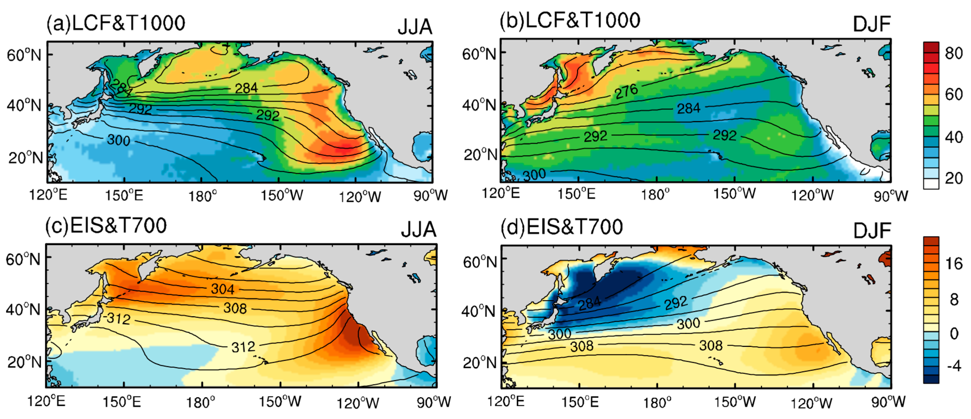
3.1. Climatological Distribution of LCF

Figure 1a,b displays the distributions of climatological LCF over the North Pacific in summer and winter, respectively. Winter is defined from December to the following February, and summer is defined from June to August. The LCF over the North Pacific is zonally inhomogeneous in both winter and summer, and exhibits obvious seasonal difference. In summer, the LCF over the eastern North Pacific is larger than that over the western North Pacific, with a local maximum around 20° N (Figure 1a). In contrast, the LCF maximum in winter appears over the western North Pacific (Figure 1b). Note that the LCF over the Bering Sea is large in both summer and winter.
Previous studies indicated that the climatological distribution of LCF and the seasonality of LCF can be well explained by the EIS, whose enhancement acts to increase LCF [42,43]. Atmospheric circulation also make contribution to the variation of LCF, such as subtropical high, Hadley–Walker circulation, and mesoscale waves [12,44]. However, EIS was proved to be the dominating factor in the seasonal variation of the LCF in previous studies [12,31]. Thus, EIS is focused on in our study. Hence, the climatological EIS defined in Equation (1) is shown in Figure 1c,d for summer and winter, respectively. Across the summertime subtropical basin (Figure 1c), the EIS is maximal off the west coast of North America around 125° W, in good correspondence with the spatial pattern of LCF (Figure 1a). Compared to the summertime situation, the EIS in winter exhibits a zonal minimum (negative center) distribution over the mid-latitude western North Pacific (Figure 1d), where a maximum LCF dominates. This is in contrast to the well-known liner relationship between EIS and LCF [13]. The enhancement of EIS could maintain a strong temperature inversion at the top of the boundary layer, inhibiting cloud-top entrainment of dry air, further contributing to LCF increase. Overall, the LCF over the eastern North Pacific is positively associated with the EIS, while the relationship between LCF and EIS over the western North Pacific is negative. Thus, the EIS alone is not sufficient to explain the observed LCF. Next, we will discuss the possible factors dominating the seasonal cycles of LCF over the eastern and western North Pacific, respectively.

3.2. Seasonal Cycle of LCF

According to previous studies, the EIS, cool advT, SHF, 700-hPa subsidence, and 700-hPa RH are the main factors affecting the formation of low-level clouds over the oceans. Overall, the enhancements of these factors contribute to LCF increase [45]. The enhancement of EIS could maintain a strong temperature inversion at the top of the boundary layer, inhibiting cloud-top entrainment of dry air, further contributing to LCF increase. The cool advT could expand the difference value between SST and SAT, further increasing SHF. The increased SHF could destabilize the surface layer, and thereby facilitate shallow convection in the boundary layer, to further increase LCF. The enhanced 700-hPa W acts to warm the mid-troposphere, inhibiting cloud-top entrainment of dry air, further increasing LCF. The 700-hPa RH could contribute to the increase of LCF by increasing the water vapor content in the air. To discuss the seasonality of LCF and its distribution over the eastern and western North Pacific, longitude-time sections of climatological LCF and the associated controlling factors along 25° N and 45° N are shown in Figure 2 and Figure 3, respectively.
These figures reveal complex relationships of LCF with its controlling factors in the course of seasonal cycles over the North Pacific. At 25° N (Figure 2a), LCF is larger in summer than in winter over the eastern subtropics (115°–135° W), which is consistent with the winter-summer difference of the EIS shown in Figure 2b. As evident in Figure 2c,d, the distributions of cold temperature advection and 700-hPa RH are also in good accordance with LCF. However, 700-hPa W and SHF are relatively weaker in summer, which is in contrary to the seasonality of LCF (Figure 2e,f). Therefore, the EIS, cold advection, and 700-hPa RH have great contributions to the enhancement of LCF over the eastern North Pacific in summer. In summer, LCF prevails over the eastern portion of the subtropical North Pacific, which is located east of the surface subtropical high that accompanies persistent mid-troposphere subsidence and equatorward surface winds. The equatorward winds induce coastal upwelling (west coast of Mexico), upper-ocean mixing, and surface evaporation, acting to maintain relatively low SST. Meanwhile, the mid-troposphere subsidence associated with the subtropical high acts to warm the mid-troposphere. The combination of cool SST and warm mid-troposphere maintains a strong temperature inversion at the top of the boundary layer, inhibiting cloud-top entrainment of dry air, further increasing LCF. Thus, the EIS can explain the summertime enhancement of LCF to a certain extent. Note that the EIS reaches its maximum in spring, while the maximum of LCF is in summer (Figure 2a,b). This may be due to both EIS and RH being large in summer, while only the EIS is large in spring. Thus, LCF reaches its maximum in summer, resulting from the combined contribution of EIS and RH, rather than in spring, when only the EIS is the strongest, suggesting the essential influence of RH on the seasonal variability of LCF over the eastern North Pacific. RH may lead to a time-lag correlation between EIS and LCF in the subtropics. The enhanced RH indicates an increase in vapor concentration in summer, which provides positive condition to the formation of low-level clouds in summer, despite the EIS being maximum in spring [46].
Figure 3 is the same as Figure 2, except along 45° N. Over the western North Pacific (145°–160° E), the EIS is larger in summer than in winter (Figure 3b), while LCF is larger in winter than in summer (Figure 3a). This is in contrast to the well-known liner relationship between EIS and LCF [47]. Meanwhile, cold advection, 700-hPa RH, 700-hPa W, and SHF are enhanced in winter over the western portion (Figure 3c–f), which is in accordance with the distribution of LCF (Figure 3a). Therefore, the wintertime enhanced LCF over the western North Pacific may be due to the enhancement of cold advection, SHF, 700-hPa W, and 700-hPa RH. On the one hand, the cold advection in winter over the western region destabilizes the surface layer, increasing the difference between SST and SAT, further resulting in large upward SHF. The wintertime enhancement of upward SHF facilitates shallow convection in the boundary layer, and further increases LCF. On the other hand, the enhanced storm track activity also contributes to the wintertime enhancement of SHF over the western North Pacific (not shown). In this area, the wintertime enhanced 700-hPa W acts to warm the mid-troposphere, inhibiting cloud-top entrainment of dry air to further increase LCF to a certain extent [20]. Moreover, similar to the situation over the eastern North Pacific, the wintertime enhancement of 700-hPa RH may also have positive effects on enhancing LCF.
As shown in the preceding section, the factors favoring increased LCF are different over the eastern and western North Pacific regions. One may question the relative importance of contributions from the EIS, advT, SHF, 700-hPa W, and 700-hPa RH to the enhancement of LCF. To further quantify their relative contributions, we reconstruct LCF using a multiple linear regression model. In this study, the regression model is constructed from climatological LCF and the factors over the eastern (115°–136° W, 15°–28° N) and western (140°–155° E, 47°–60° N) North Pacific, respectively. To describe the relative importance of cloud controlling factors, the annual mean has been removed. The regression slope of LCF variation against each predictor is given in Table 1.
Figure 4 and Figure 5 show the longitude-time distributions of the predicted climatological seasonal cycles# of LCF along 25° N and 45° N, respectively. Besides, the corresponding LCF predicted by the multiple linear regression model is also shown in Figure 4b and Figure 5b, named “Total”. At 25° N, the multiple linear regression model explains 71% of the total variance of LCF regionality and its seasonal cycle, whereas the root mean square error (RMSE) between observed and predicted LCF is 8%. The model reproduces the summertime LCF maximum from July to September over the eastern subtropics (Figure 4a,b). The reconstruction indicates that the EIS (Figure 4c) and RH (Figure 4e) make the greatest contributions to the summertime enhancement of LCF, and the contribution from cold advection is also important (Figure 4d). In contrast, the 700-hPa W and SHF act to reduce LCF in summer (Figure 4f,g).
At 45° N, the reconstructed LCF can also reproduce LCF well. In this area, the reconstruction explains 68% of the total variance of LCF, and the RMSE between observed and predicted LCF is 9% (Figure 5a,b). The wintertime LCF enhancement over the western North Pacific is mostly attributable to enhanced cold advection and SHF (Figure 5d,g). Nevertheless, the EIS in this area acts to suppress the wintertime enhancement of LCF (Figure 5c), and the direct impacts of 700-hPa RH and W are negligible (Figure 5e,f).
Overall, the dominating factors associated with the seasonal cycle of LCF are different over the eastern and western North Pacific regions. Over the eastern North Pacific, the EIS dominates the enhancement of LCF in summer, together with the 700-hPa RH. Over the western North Pacific, the enhancement of LCF in winter is mostly due to enhanced SHF and cold advection.

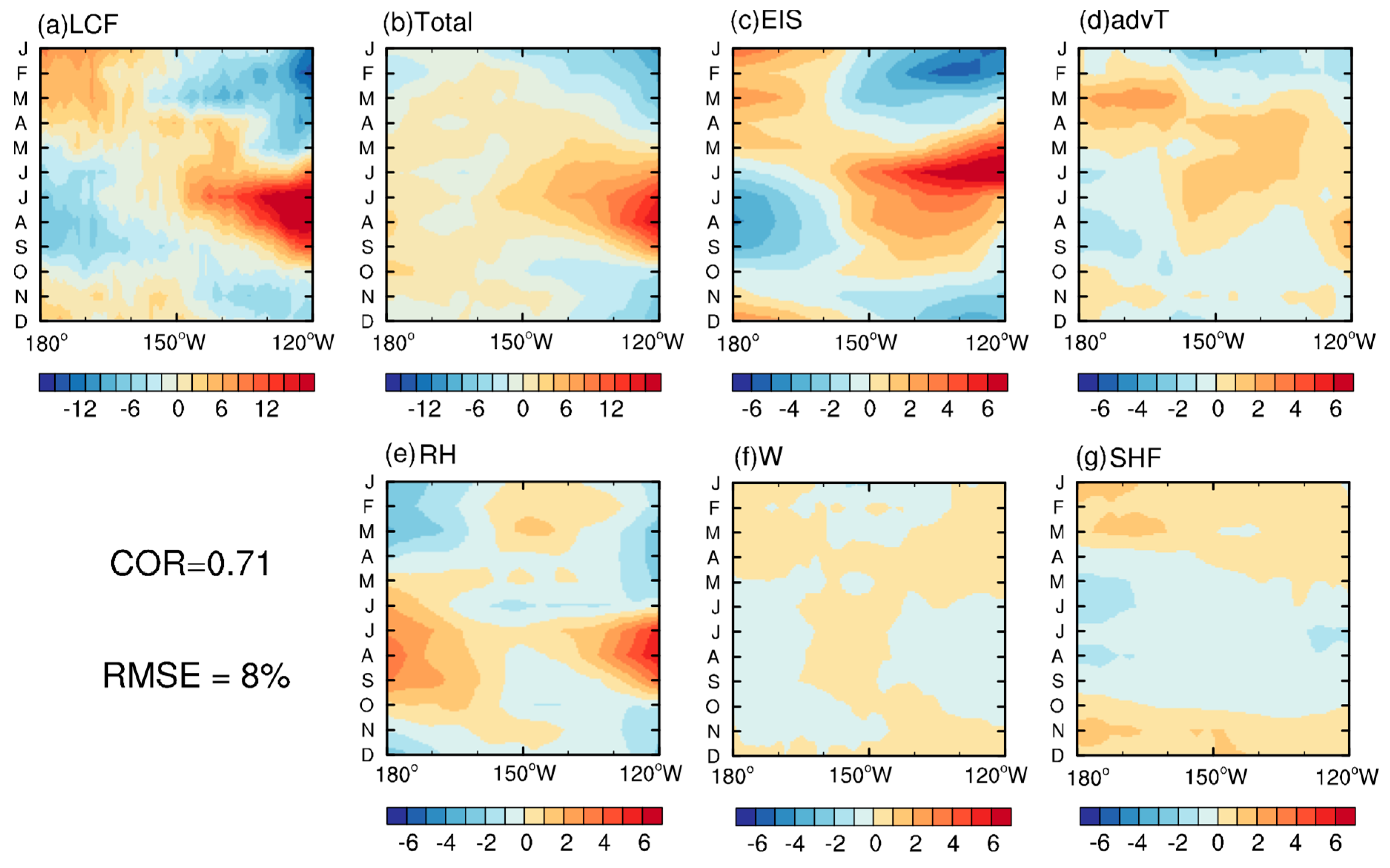
3.3. Association with Meteorological Parameters

In this subsection, we examine the interannual variability of EIS, 700-hPa W, advT, SHF, and SST to investigate the possible factors associated with the interannual variability of LCF over eastern and western North Pacific regions, respectively. We calculated the interannual variance of LCF in different seasons. We first choose three regions over the eastern North Pacific where the variances are large. However, in order to investigate the different factors of LCF between eastern and western North Pacific, we also choose three regions over the western North Pacific where the variances of LCF are also large (Figure 6). The six different regions are defined as follows: the Okhotsk Sea (OS; 140°–155° E, 47°–60° N), the Kuroshio Extension (KE; 142°–180° E, 37°–44° N), the south basin of Japan (SJ; 124°–145° E, 25°–31° N), the center of the North Pacific (CE; 136°–165° W, 26°–37° N), the southeastern North Pacific (SE; 115°–136° W, 15°–28° N), and the northeastern North Pacific (NE; 124°–148° W, 26°–43° N).
First, we calculated the correlation coefficients between regional-mean LCF and corresponding meteorological variables for each region. Table 2 lists these correlation coefficients. For the correlation coefficients of different regions and seasons, we use the method of significance test of correlation coefficients [48]. According to the significance test table of correlation coefficient, we can see that when the degree of freedom n = 11, the correlation coefficient (COR) which is larger than 0.553 (COR < −0.553) exceeds a 95% confidence level; the COR which is less than 0.476 (−0.476 < COR < 0) cannot exceed a 90% confidence level.
Over the eastern portions (SE, NE, and CE), the LCF is positively correlated with the EIS and negatively correlated with the SST, especially in summer and winter; the 700-hpa W also plays a positive role in the interannual variation of LCF over the eastern portions. In NE and CE, there is a positive correlation between LCF and cold advection. Over the eastern portions, the correlation between LCF and SHF is not obvious.
In contrast to the eastern regions, the correlations between LCF and meteorological parameters over the western regions (OS, KE, and SJ) present radically different features. Over the western regions, the LCF is positively connected with cold advection and SHF, especially in winter and spring. Note that there is no relationship between LCF and EIS, or between LCF and SST. Over the western regions, the 700-hPa W also has a positive correlation with LCF, similar to that in the eastern regions.
These correlation coefficients reflect regional contrast at the interannual time scale. The LCF over the eastern North Pacific is positively correlated with both EIS and SST; the LCF over the western regions coincides well with SHF and cold advection. The 700-hPa W has positive relation with LCF over both western and eastern regions.

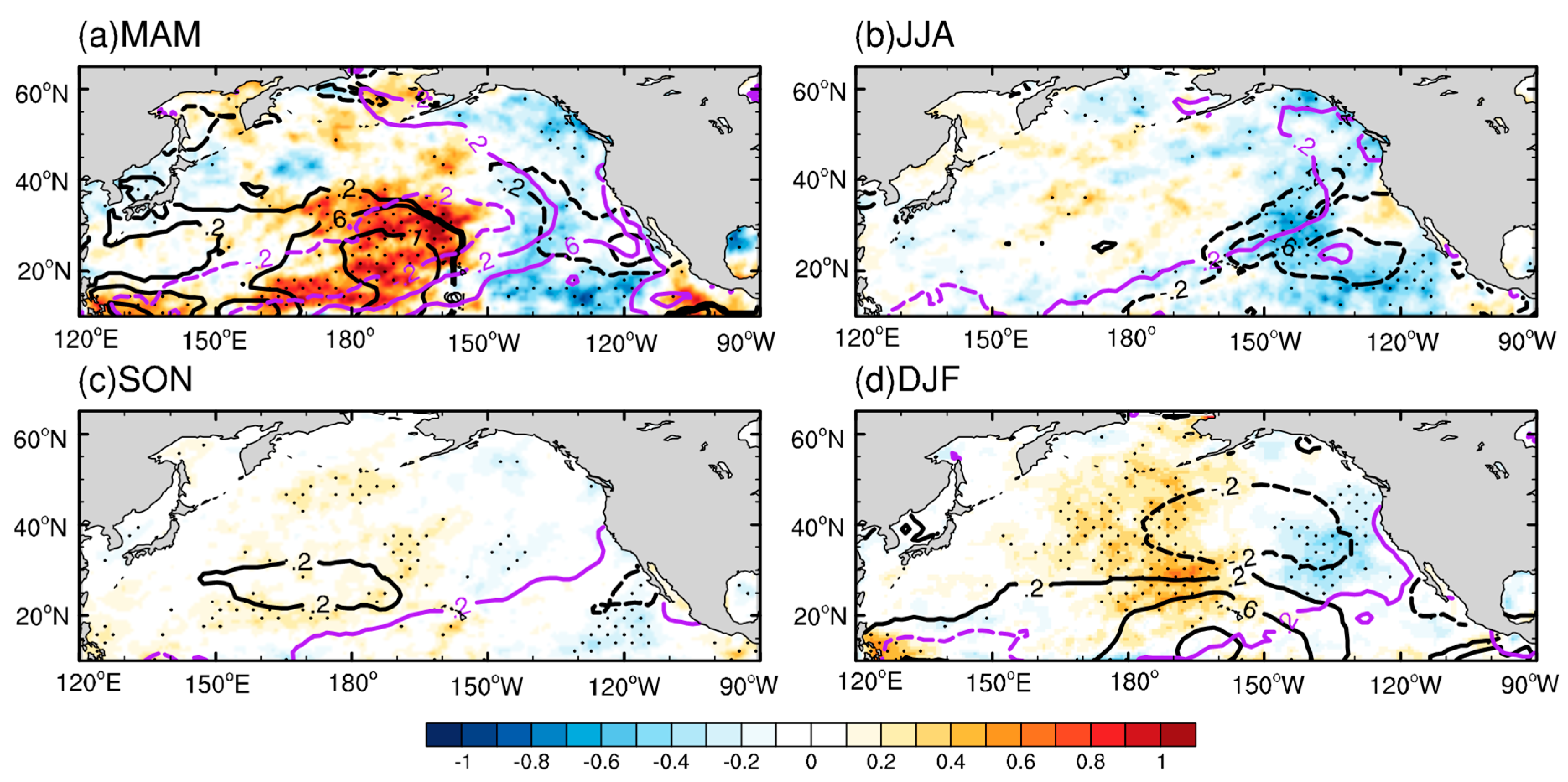
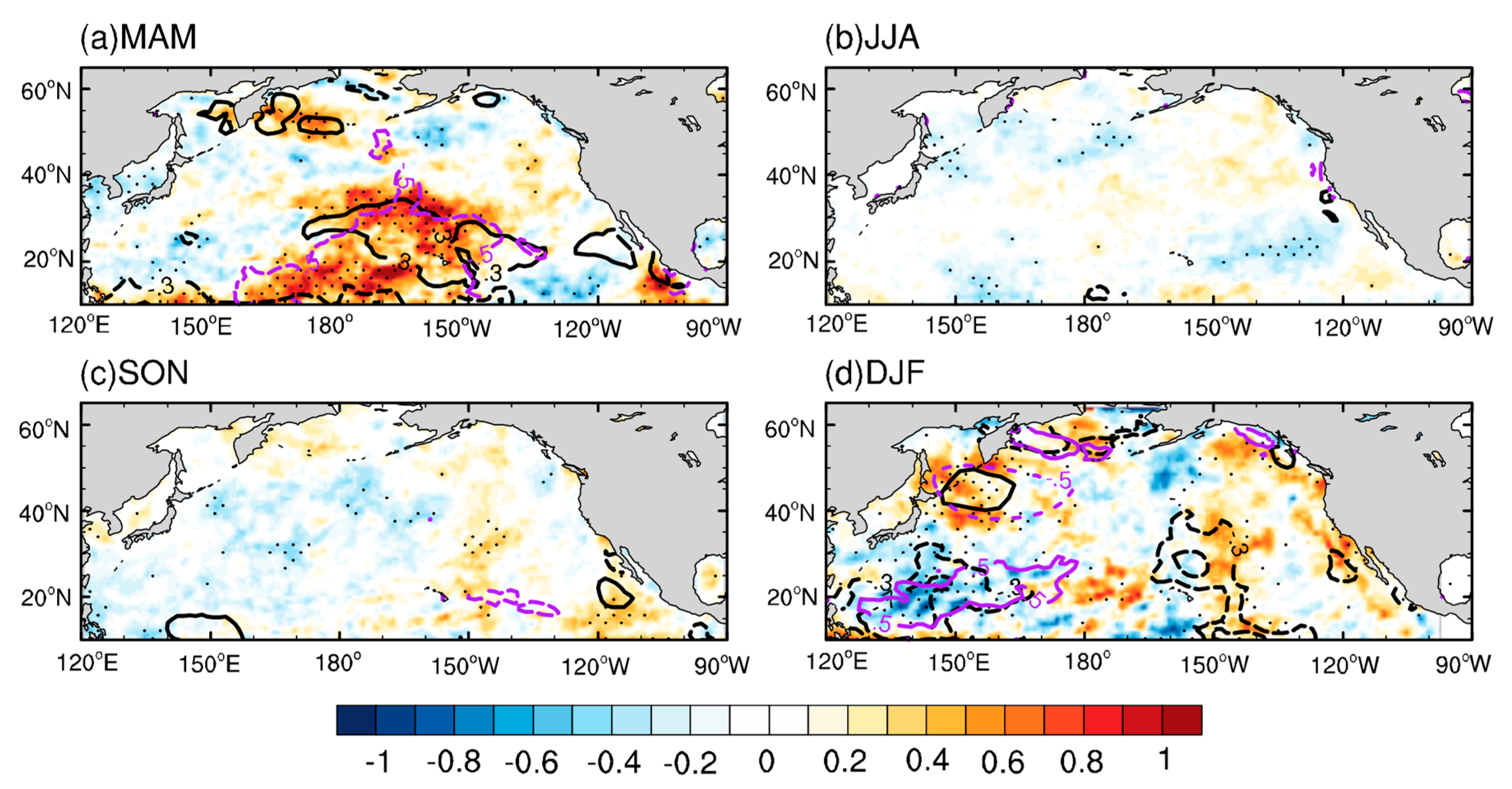
3.4. Association with El Niño and SPFZ

What causes the characteristic interannual variations in SST, EIS, advT, and SHF, which are closely linked with the interannual variation of LCF? In this subsection, we first discuss the possible relationship of LCF with the El Niño, which is the primary variability in the North Pacific at the interannual time scale. Figure 7 shows the interannual anomalies of LCF, SST, and EIS over the North Pacific regressed onto the synchronization Niño-3.4 index in different seasons. Usually, the El Niño occurs in the eastern equatorial Pacific. Warm SST anomalies simultaneously occur in the surrounding regions (Figure 7a–d), which are well-known as the typical SST anomaly distribution associated with the El Niño [49,50]. Meanwhile, the warm SST benefits warm surface potential temperature, corresponding to the overlying negative EIS. This is consistent with the negative correlation between EIS and El Niño over the eastern North Pacific. The negative EIS over the eastern North Pacific favors negative LCF. Thus, El Niño-related SSTs have negative feedback on the LCF over the eastern North Pacific, in which the EIS plays an important role. This is consistent with the results of previous studies [51].
The LCF over the western North Pacific does not have a clear relationship with the El Niño. This begs the question: Is there any possible link with other climate modes? From Table 2, we can see that the LCF over the western North Pacific is positively related to cold advection and SHF. Thus, in Figure 8, we show the maps of LCF, advT, and SHF anomalies regressed onto the normalized subpolar frontal zone (SPFZ) index, similar to Figure 7. The interannual LCF anomalies are positively correlated with the intensity of the SPFZ over the western North Pacific (140°–170° W, 40°–60° N), especially in winter and spring (Figure 8a,d). At the same time, both cold advection and SHF present positive correlations with the SPFZ (Figure 8a,d). In spring and winter, the enhancement of the SPFZ over the western North Pacific can strengthen the cold advection through northerly wind, rendering SAT lower than the SST underneath, further resulting in large upward SHF [52]. The wintertime enhancement of SHF destabilizes the surface layer and facilitates shallow convection in the boundary layer, thus increasing the convective LCF. This implies that the SPFZ-related cold advection has a positive effect on the enhanced LCF by interacting with the SHF over the western North Pacific.
Overall, the interannual variation of LCF is different over the eastern and western North Pacific regions, due to different controlling factors and large-scale atmospheric processes. The increased LCF over the eastern North Pacific is associated with increased EIS and decreased SST, especially in summer. Our regression analysis signifies the El Niño contribution. Over the western North Pacific, the springtime and wintertime enhanced LCF has a positive correlation with enhanced SHF and cold advection, which can be partly explained by SPFZ intensity.

4. Discussion and Concluding

In this study, we investigate the seasonal and interannual variability of LCF and associated controlling factors over the eastern and western North Pacific. On the seasonal time scale, LCF shows obvious regional contrast. Over the eastern North Pacific, the EIS dominates the enhancement of LCF in summer, together with the 700-hPa RH. Over the western North Pacific, the enhancement of LCF in winter is mostly due to enhanced SHF and surface cold advection.
In terms of interannual variation, the increased LCF over the eastern North Pacific is associated with increased EIS and decreased SSTs, especially in summer. Our regression analysis indicates that El Niño contributes most. Over the western North Pacific, the springtime and wintertime enhanced LCF has a positive correlation with enhanced SHF and cold advection, which can be partly explained by SPFZ intensity.
This paper only discusses the factors that influence LCF variability in previous work. However, other factors, such as ocean or atmospheric circulation, may also play an important role in LCF changes, which need to be further studied in the future. Cloud microphysical processes and aerosol properties are also important for the formation of low-level clouds [53]. For example, oceanic aerosol productivity plays an important role in determining cloud condensation nuclei. Zhao et al. have found that if liquid water content (LWC) is high and aerosol amount is not too large, both cloud droplet number concentration (N) and effective radius (re) increase with increasing aerosols; if LWC is low or if LWC is high but aerosol amount is too large, cloud N increases but re decreases with increasing aerosols [54]. These aspects will be explored in our future study.

Author Contributions

Conceptualization, H.X. Formal analysis, Q.W. Methodology, Q.W., H.X. and L.Z. Software, Q.W. Supervision, H.X. Validation, Q.W. and L.Z. Writing—original draft, Q.W. and L.Z. Writing—review and editing, Q.W., H.X., L.Z. and J.D.

Funding

This work was jointly supported by the Natural Science Foundation of China (41575077, 41490643, and 41705054), and the Priority Academic Program Development of Jiangsu Higher Education Institutions (PAPD). Deng was supported by the Natural Science Foundation of Jiangsu Province (BK20170942), the General Program of Natural Science Research of Jiangsu Province University (17KJB170012), and the China Scholarship Council (CSC).

Conflicts of Interest

The authors declare no conflict of interest.

References

  1. Wood, R. Stratocumulus Clouds. Mon. Weather Rev. 2012, 140, 2373–2423. [Google Scholar] [CrossRef]
  2. Garrett, T.J.; Zhao, C. Increased Arctic cloud longwave emissivity associated with pollution from mid-latitudes. Nature 2006, 440, 787. [Google Scholar] [CrossRef] [PubMed]
  3. Zhao, C.; Garrett, T.J. Effects of Arctic haze on surface cloud radiative forcing. Geophys. Res. Lett. 2015, 42, 557–564. [Google Scholar] [CrossRef] [Green Version]
  4. Randall, D.A.; Coakley, J.A., Jr.; Fairall, C.W.; Kropfli, R.A.; Lenschow, D.H. Outlook for research on subtropical marine stratiform clouds. Bull. Am. Meteorol. Soc. 1984, 65, 1290–1301. [Google Scholar] [CrossRef]
  5. Oreopoulos, L.; Davies, R. Statistical dependence of albedo and cloud cover on sea surface temperature for two tropical marine stratocumulus regions. J. Clim. 1993, 6, 2434–2447. [Google Scholar] [CrossRef]
  6. Ma, Z.; Liu, Q.; Zhao, C.; Shen, X.; Wang, Y.; Jiang, J.H.; Li, Z.; Yung, Y. Application and Evaluation of an Explicit Prognostic Cloud-Cover Scheme in GRAPES Global Forecast System. J. Adv. Model. Earth Syst. 2018, 10, 652–667. [Google Scholar] [CrossRef] [Green Version]
  7. Fan, T.; Zhao, C.; Dong, X.; Liu, X.; Yang, X.; Zhang, F.; Shi, C.; Wang, Y.; Wu, F. Quantify contribution of aerosol errors to cloud fraction biases in CMIP5 Atmospheric Model Intercomparison Project simulations. Int. J. Climatol. 2018, 38, 3140–3156. [Google Scholar] [CrossRef]
  8. Bony, S.; Dufresne, J.L. Marine boundary layer clouds at the heart of tropical cloud feedback uncertainties in climate models. Geophys. Res. Lett. 2005, 32, 023851. [Google Scholar] [CrossRef]
  9. Zhai, C.; Jiang, J.H.; Su, H. Long-term cloud change imprinted in seasonal cloud variation: More evidence of high climate sensitivity. Geophys. Res. Lett. 2015, 42, 8729–8737. [Google Scholar] [CrossRef]
  10. Trenberth, K.E.; Fasullo, J.T. Simulation of present-day and twenty-first-century energy budgets of the southern oceans. J. Clim. 2010, 23, 440–454. [Google Scholar] [CrossRef]
  11. Grise, K.M.; Polvani, L.M.; Fasullo, J.T. Re-examining the relationship between climate sensitivity and the southern hemisphere radiation budget in cmip models. J. Clim. 2015, 28. [Google Scholar] [CrossRef]
  12. Koshiro, T.; Yukimoto, S.; Shiotani, M. Interannual variability in low stratiform cloud amount over the summertime North Pacific in terms of cloud types. J. Clim. 2017, 30, 6107–6121. [Google Scholar] [CrossRef]
  13. Wood, R.; Bretherton, C.S. On the relationship between stratiform low cloud cover and lower-tropospheric stability. J. Clim. 2006, 19, 6425–6432. [Google Scholar] [CrossRef]
  14. Klein, S.A.; Hartmann, D.L. The seasonal cycle of low stratiform clouds. J. Clim. 1993, 6, 1587–1606. [Google Scholar] [CrossRef]
  15. Myers, T.A.; Norris, J.R. Observational evidence that enhanced subsidence reduces subtropical marine boundary layer cloudiness. J. Clim. 2013, 26, 7507–7524. [Google Scholar] [CrossRef]
  16. Miyasaka, T.; Nakamura, H. Structure and formation mechanisms of the northern hemisphere summertime subtropical highs. J. Clim. 2005, 18, 5046–5065. [Google Scholar] [CrossRef]
  17. Deser, C.; Wahl, S.; Bates, J.J. The influence of sea surface temperature gradients on stratiform cloudiness along the equatorial front in the Pacific Ocean. J. Clim. 1993, 6, 1172–1180. [Google Scholar] [CrossRef]
  18. Dong, S.; Gille, S.T.; Sprintall, J. An assessment of the Southern Ocean mixed layer heat budget. J. Clim. 2007, 20, 4425–4442. [Google Scholar] [CrossRef]
  19. Bretherton, C.S.; Blossey, P.N.; Jones, C.R. Mechanisms of marine low cloud sensitivity to idealized climate perturbations: A single-les exploration extending the cgils cases. J. Adv. Model. Earth Syst. 2013, 5, 316–337. [Google Scholar] [CrossRef]
  20. Garrett, T.J.; Zhao, C.; Dong, X.; Mace, G.G.; Hobbs, P.V. Effects of varying aerosol regimes on low-level Arctic stratus. Geophys. Res. Lett. 2004, 31. [Google Scholar] [CrossRef]
  21. Zhao, C.; Chen, Y.; Li, J.; Letu, H.; Su, Y.; Chen, T.; Wu, X. Fifteen-year statistical analysis of cloud characteristics over China using Terra and Aqua Moderate Resolution Imaging Spectroradiometer observations. Int. J. Climatol. 2018. [Google Scholar] [CrossRef]
  22. Seethala, C.; Norris, J.R.; Myers, T.A. How has subtropical stratocumulus and associated meteorology changed since the 1980s? J. Clim. 2015, 28. [Google Scholar] [CrossRef]
  23. Tselioudis, G.; Rossow, W.B.; Rind, D. Global patterns of cloud optical thickness variation with temperature. J. Clim. 1992, 5, 1484–1495. [Google Scholar] [CrossRef]
  24. Van der Dussen, J.J.; De Roode, S.R.; Dal Gesso, S.; Siebesma, A.P. An les model study of the influence of the free tropospheric thermodynamic conditions on the stratocumulus response to a climate perturbation. J. Adv. Model. Earth Syst. 2015, 7, 670–691. [Google Scholar] [CrossRef]
  25. Norris, J.R.; Leovy, C.B. Interannual variability in stratiform cloudiness and sea surface temperature. J. Clim. 1994, 7, 1915–1925. [Google Scholar] [CrossRef]
  26. Norris, J.R. On trends and possible artifacts in global ocean cloud cover between 1952 and 1995. J. Clim. 1999, 12, 1864–1870. [Google Scholar] [CrossRef]
  27. Norris, J.R. Interannual and interdecadal variability in the storm track, cloudiness, and sea surface temperature over the summertime North Pacific. J. Clim. 2000, 13, 422–430. [Google Scholar] [CrossRef]
  28. Remer, L.A.; Kaufman, Y.J.; Tanré, D.; Mattoo, S.; Chu, D.A.; Martins, J.V. The modis aerosol algorithm, products, and validation. J. Atmos. Sci. 2005, 62, 947–973. [Google Scholar] [CrossRef]
  29. Wang, Y.; Zhao, C. Can MODIS cloud fraction fully represent the diurnal and seasonal variations at DOE ARM SGP and Manus sites? J. Geophys. Res. Atmos. 2017, 122, 329–343. [Google Scholar] [CrossRef]
  30. Ackerman, S.A.; Strabala, K.I.; Menzel, W.P.; Frey, R.A.; Moeller, C.C.; Gumley, L.E. Discriminating clear sky from clouds with modis. J. Geophys. Res. 1998, 103, 32141. [Google Scholar] [CrossRef]
  31. Miyamoto, A.; Nakamura, H.; Miyasaka, T. Influence of the subtropical high and storm track on low-cloud fraction and its seasonality over the south Indian Ocean. J. Clim. 2018, 31, 4017–4039. [Google Scholar] [CrossRef]
  32. Weare, B.C. Near-global observations of low clouds. J. Clim. 2000, 13, 1255–1268. [Google Scholar] [CrossRef]
  33. McCoy, D.T.; Burrows, S.M.; Wood, R.; Grosvenor, D.P.; Elliott, S.M.; Ma, P.L.; Hartmann, D.L. Natural aerosols explain seasonal and spatial patterns of Southern Ocean cloud albedo. Sci. Adv. 2015, 1, e1500157. [Google Scholar] [CrossRef] [PubMed] [Green Version]
  34. Li, J.; Huang, J.; Stamnes, K.; Wang, T.; Lv, Q.; Jin, H. A global survey of cloud overlap based on calipso and cloudsat measurements. Atmos. Chem. Phys. 2015, 15, 519–536. [Google Scholar] [CrossRef]
  35. Dee, D.P.; Uppala, S.M.; Simmons, A.J.; Berrisford, P.; Poli, P.; Kobayashi, S.; Bechtold, P. The ERA-Interim reanalysis: Configuration and performance of the data assimilation system. Q. J. R. Meteorol. Soc. 2011, 137, 553–597. [Google Scholar] [CrossRef]
  36. Wei, W.; Li, W.; Deng, Y.; Yang, S.; Liu, W.T. Dynamical and thermodynamical coupling between the north atlantic subtropical high and the marine boundary layer clouds in boreal summer. Clim. Dyn. 2017, 19, 1–13. [Google Scholar] [CrossRef]
  37. Yu, L.; Weller, R.A. Objectively analyzed air–sea heat fluxes for the global ice-free oceans (1981–2005). Bull. Am. Meteorol. Soc. 2007, 88, 527–539. [Google Scholar] [CrossRef]
  38. Bunge, L.; Clarke, A.J. A verified estimation of the El Niño index Niño-3.4 since 1877. J. Clim. 2009, 22, 3979–3992. [Google Scholar] [CrossRef]
  39. Klein, S.A.; Hartmann, D.L.; Norris, J.R. On the relationships among low-cloud structure, sea surface temperature, and atmospheric circulation in the summertime northeast pacific. J. Clim. 1995, 8, 2063–2078. [Google Scholar] [CrossRef]
  40. Norris, J.R.; Iacobellis, S.F. North pacific cloud feedbacks inferred from synoptic-scale dynamic and thermodynamic relationships. J. Clim. 2005, 18, 4862–4878. [Google Scholar] [CrossRef]
  41. Mansbach, D.K.; Norris, J.R. Low-level cloud variability over the equatorial cold tongue in observations and models. J. Clim. 2007, 20, 1555–1570. [Google Scholar] [CrossRef]
  42. Yao, Y.; Zhong, Z.; Yang, X.Q. Impacts of the subarctic frontal zone on the North Pacific storm track in the cold season: An observational study. Int. J. Climatol. 2018, 38, 2554–2564. [Google Scholar] [CrossRef]
  43. Qu, X.; Hall, A.; Klein, S.A.; Deangelis, A.M. Positive tropical marine low-cloud cover feedback inferred from cloud-controlling factors. Geophys. Res. Lett. 2015, 42, 7767–7775. [Google Scholar] [CrossRef]
  44. Bony, S.; Stevens, B.; Frierson, D.M.; Jakob, C.; Kageyama, M.; Pincus, R.; Shepherd, G. Clouds, circulation and climate sensitivity. Nat. Geosci. 2015, 8, 261–268. [Google Scholar] [CrossRef]
  45. Koshiro, T.; Shiotani, M. Relationship between low stratiform cloud amount and estimated inversion strength in the lower troposphere over the global ocean in terms of clouds. J. Meteorol. Soc. Jpn. Ser. II 2014, 92, 107–120. [Google Scholar] [CrossRef]
  46. Eastman, R.; Warren, S.G.; Hahn, C.J. Variations in cloud cover and cloud types over the ocean from surface observations, 1954–2008. J. Clim. 2011, 24, 5914–5934. [Google Scholar] [CrossRef]
  47. Xu, H.; Xie, S.P.; Wang, Y. Subseasonal variability of the southeast Pacific stratus cloud deck. J. Clim. 2005, 18, 131–142. [Google Scholar] [CrossRef]
  48. Van der Dussen, J.J.; De Roode, S.R.; Ackerman, A.S.; Blossey, P.N.; Bretherton, C.S.; Kurowski, M.J.; Lock, A.P. The gass/euclipse model intercomparison of the stratocumulus transition as observed during astex: Les results. J. Adv. Model. Earth Syst. 2013, 5, 483–499. [Google Scholar] [CrossRef]
  49. Lau, N.C.; Nath, M.J. Impact of ENSO on SST variability in the north pacific and north atlantic: Seasonal dependence and role of extratropical sea–air coupling. J. Clim. 2001, 14, 2846–2866. [Google Scholar] [CrossRef]
  50. Zhu, P.; Hack, J.J.; Kiehl, J.T.; Bretherton, C.S. Climate sensitivity of tropical and subtropical marine low cloud amount to ENSO and global warming due to doubled CO2. J. Geophys. Res. Atmos. 2007, 112. [Google Scholar] [CrossRef]
  51. Park, S.; Leovy, C.B. Marine low-cloud anomalies associated with ENSO. J. Clim. 2004, 17, 3448–3469. [Google Scholar] [CrossRef]
  52. Lana, A.; Bell, T.G.; Simó, R.; Vallina, S.M.; Ballabrera-Poy, J.; Kettle, A.J.; Johnson, J.E. An updated climatology of surface dimethlysulfide concentrations and emission fluxes in the global ocean. Glob. Biogeochem. Cycles 2011, 25. [Google Scholar] [CrossRef] [Green Version]
  53. Zhao, C.; Qiu, Y.; Dong, X.; Wang, Z.; Peng, Y.; Li, B.; Wu, Z.; Wang, Y. Negative Aerosol-Cloud re Relationship from Aircraft Observations Over Hebei, China. Earth Space Sci. 2018, 5, 19–29. [Google Scholar] [CrossRef]
  54. Yang, Y.; Zhao, C.; Dong, X.; Fan, G.; Zhou, Y.; Wang, Y.; Zhao, L.; Lv, F.; Yan, F. Toward understanding the process-level impacts of aerosols on microphysical properties of shallow cumulus cloud using aircraft observations. Atmos. Res. 2019. [Google Scholar] [CrossRef]
Figure 1. Climatological low-cloud fraction (LCF; shading; units: %) and surface potential temperature (contour interval: 2 K) in summer (a) and in winter (b); (c,d) are the same as (a,b), but for estimated inversion strength (EIS; shading; units: K) and 700-hPa potential temperature (contour interval: 4 K).
Atmosphere 10 00126 g001
Figure 2. Time-longitude section of climatological (a) LCF (shading; units: %), (b) EIS (shading; units: K), (c) near-surface temperature advection (advT; shading; units: K/day), (d) 700-hPa relative humidity (RH; shading; units: %), (e) 700-hPa subsidence (W; shading; units: m/s), and (f) sensible heat flux (SHF; shading; units: W/m2) along 25° N.
Atmosphere 10 00126 g002
Figure 3. Time-longitude section of climatological (a) LCF (shading; units: %), (b) EIS (shading; units: K), (c) near-surface advT (shading; units: K/day), (d) 700-hPa RH (shading; units: %), (e) 700-hPa W (shading; units: m/s), and (f) SHF (shading; units: W/m2) along 45° N.
Atmosphere 10 00126 g003
Figure 4. (a) Same as Figure 2a, except that the annual-mean LCF (%) has been removed. (b) Same as (a), except for the corresponding LCF (%) predicted by the multiple linear regression model. The correlation and root mean square error (RMSE) between (a,b) are shown below (a). (cg) Same as (b), except for individual contributions from EIS, advT, 700-hPa RH, 700-hPa subsidence, and SHF to (b), respectively.
Atmosphere 10 00126 g004
Figure 5. (a) Same as Figure 3a, except that the annual-mean LCF (%) has been removed. (b) Same as (a), except for the corresponding LCF (%) predicted by the multiple linear regression model. The correlation and root mean square error (RMSE) between (a,b) are shown below (a). (cg) Same as (b), except for individual contributions from EIS, advT, 700-hPa RH, 700-hPa subsidence, and SHF to (b), respectively.
Atmosphere 10 00126 g005
Figure 6. Interannual LCF variance (shading; units: %2) in (a) spring, (b) summer, (c) autumn, and (d) winter. Thick solid rectangles designate different regions discussed in Section 4.
Atmosphere 10 00126 g006
Figure 7. Coefficients of interannual LCF (shading; units: %), SST (purple contour; units: K), and EIS (black contour; units: K) onto the synchronization Niño-3.4 index for (a) spring, (b) summer, (c) autumn, and (d) winter. Stippling indicates the 90% confidence level using the t test. Contours indicate statistically significant positive (solid) and negative (dashed) differences.
Atmosphere 10 00126 g007
Figure 8. Regression coefficients of interannual LCF (shading; units: %), advT (purple contour; units: K/day), and SHF (black contour; units: W/m2) onto the SPFZ index for (a) spring, (b) summer, (c) autumn, and (d) winter. Stippling indicates the 90% confidence level using the t test. Contours indicate statistically significant positive (solid) and negative (dashed) differences at the 90% confidence level based on the t test.
Atmosphere 10 00126 g008
Table 1. Regression slope for each predictor (EIS: estimated inversion strength; advT: surface temperature advection; SHF: sensible heat flux; W: 700-hPa subsidence; RH: 700-hPa relative humidity).
Area∂LCF/∂EIS (% K−1)∂LCF/∂advT (%(Kday−2)−1)∂LCF/∂SHF (%(Wm−2)−1)∂LCF/∂W (%(m−1)−1)∂LCF/∂RH (%%−1)
Western North Pacific−0.08−0.190.1248.6−0.14
Eastern North Pacific0.47−2.860.1658.890.27
Table 2. Correlation coefficients of regionally-averaged interannual anomalies of various meteorological parameters with those of LCF. The bold type exceed a 95% confidence level, while the parentheses indicate that the correlation coefficient is not statistically significant. (SE: the southeastern North Pacific; NE: the northeastern North Pacific; CE: the center of the North Pacific; OS: the Okhotsk Sea; KE: the Kuroshio Extension; SJ: the south basin of Japan).
AreaSeasonEstimated
Inversion
Strength
(EIS)
700-hPa
Subsidence
(W)
Surface
Temperature
Advection
(advT)
Sensible
Heat Flux
(SHF)
Sea
Surface
Temperature
(SST)
SESpring0.49(−0.25)(0.04)(−0.24)(−0.41)
Summer0.57−0.64(−0.11)(−0.07)−0.57
Autumn (0.36)(0.04)(−0.07)−0.61−0.72
Winter 0.55−0.65(0.12)(0.21)(−0.43)
NESpring(0.25)−0.51−0.73(0.46)−0.64
Summer0.73−0.60(−0.38)(−0.39)−0.74
Autumn0.56(−0.45)−0.66(−0.02)(−0.12)
Winter0.57−0.81−0.850.54−0.57
CESpring0.71−0.91−0.810.68(−0.37)
Summer0.71(−0.41)(−0.37)(0.42)−0.59
Autumn0.59−0.81(−0.29)(0.001)(−0.25)
Winter0.60−0.84−0.48(0.40)(0.35)
OSSpring(−0.34)(−0.41)(0.05)(0.15)(0.07)
Summer(0.07)(−0.35)(0.16)0.51(−0.24)
Autumn−0.48(−0.35)(−0.35)(0.39)(−0.37)
Winter(−0.36)−0.58−0.650.61(0.02)
KESpring(−0.16)−0.59−0.560.61(−0.08)
Summer(0.21)(−0.42)−0.620.67(−0.05)
Autumn(−0.28)(−0.32)−0.48(0.27)(0.02)
Winter(−0.30)−0.62−0.60(0.45)(−0.43)
SJSpring(−0.01)(−0.22)(−0.17)(0.38)(−0.10)
Summer(−0.24)−0.55(0.13)(0.31)(0.21)
Autumn(0.37)−0.47(−0.09)0.56(−0.21)
Winter(−0.18)−0.80−0.70.65−0.85

