Long-Term Observed Visibility in Eastern Thailand: Temporal Variation, Association with Air Pollutants and Meteorological Factors, and Trends

Abstract

The present study analyzed long-term observed visibility over Eastern Thailand, with a focus on urbanized/highly industrialized coastal areas. The temporal coverage spans 9 to 35 years for visibility data and 9 to 15 years for air quality data for the selected stations. Visibility shows strong seasonality and its degradation intensifies in the dry season. It shows a negative correspondence with PM₁₀ and relative humidity, which is evident from different methods. Visibility has strong dependence on wind direction, suggesting the influence of local pollution sources. Back-trajectory results suggest important influences of long-range transport and humidity. Secondary aerosol formation has the potential to aggravate visibility based on a precursor-ratio method. The trends in average visibility at most stations in recent years show negative shift, decreasing direction, or persistence of relatively low visibility, possibly due to increase in air pollution. Contrast was found in the meteorologically adjusted trend (based on generalized linear models) in visibility and PM₁₀, which is partly attributed to the role of fine particles. The study suggests that visibility degradation is a problem in Eastern Thailand and is affected by both air pollutants and meteorology. The study hopes to get attention from policymakers regarding issue of visibility degradation in the region.

1. Introduction

The horizontal distance over which a human can observe and distinguish a dark object (or an object with sufficient visual contrast to the background) is termed as visibility or visual range [1,2]. It is a fundamental parameter routinely observed at standard surface weather stations. Visibility is governed by optical properties of airborne particles and gases (apart from light intensity), physical properties of the target, and the threshold visual contrast of the observer. In a clean environment (in the absence of fog), visibility can be reduced mainly by molecular (i.e., Rayleigh) scattering and gas absorption; however, in a polluted environment, scattering and absorption of light by both particles and gases can reduce visibility [3,4]. Thus, visibility is linked to air pollution and indicates its extent, especially for long-term studies when air quality data are unavailable [5,6,7,8,9]. Severe reduction of visibility can interfere with or disrupt transportation (e.g., traffic slowdown, delayed flights, and on-road accidents) and also discourage recreational activities and tourism [1]. Visibility is also dependent on several meteorological factors [10,11,12]. Most atmospheric aerosols are hygroscopic [6] (especially sea salt, and carbonaceous and inorganic aerosols), that is, they absorb water; this absorption in turn increases aerosol size and thus increases the light scattering [1]. The transport of pollutants from remote sources by winds and secondary aerosols through complex multi-phase atmospheric chemistry (especially inorganic components such as sulfate, nitrate, and ammonia) can enhance the visibility reduction over an area in addition to local pollutants emitted within the area [13].

Numerous studies have been done to understand visibility characterization and factors affecting it at both local and global scales. Wang et al. (2009) [14] reported an increasing trend for visibility since the mid-1980s in Europe and North America, while the trend was found to be decreasing over South and East Asia, South America, Australia, and Africa. Another study by Wang et al. (2012) [15] showed that, in spite of decreasing levels of PM₁₀ (particulate matter with a size smaller than or equal to 10 µm) across the world, optical extinction has either increased or shown less decrease. Hu et al. (2017) [16] studied the visibility trend in selected cities in the USA, India, and China during 1973–2015, and reported that visibility has improved in the USA and China (after an initial decrease until the 1990s) but was still a concern in India. Moreover, Singh et al. (2017) [6] reported an increasing trend in visibility over the UK. Overall, it can be said that visibility has mostly improved in developed countries over the last few decades but that it is still a concern over developing countries due to rapid economic development [7,10,16,17]. The impact of meteorological factors on visibility has also been reported in many studies [4,6,7,8,9,10,11,12,13].

Industrialization and urbanization in many areas across Thailand have resulted in a number of environmental issues, one of which is air pollution problems in the eastern region [18,19,20,21,22,23]. Currently, the region comprises seven provinces (Chon Buri, Rayong, Chanthaburi, Trat, Prachin Buri, Sa Kaeo, and Chachoengsao) (Figure 1a,b), with the first two being the most industrialized provinces in the country. Eastern Thailand is economically important, accounting for 18% of national gross domestic product (GDP) (as of 2015), second only to the Bangkok Metropolitan Region (47%) [24]. In view of gross provincial product (GPP) (which is the same as GDP but scaled to a provincial level) and fuel consumption, Chon Buri and Rayong provinces both have an apparent growth, particularly after 1990 (although with a single drop in 2009 caused by the impact of the global financial crisis), and each has shown an overall positive population growth since 1981 [25,26] (Figure 2). Eastern Thailand is also well known for many tourist attractions (beaches, islands, national parks, eco-tourism, and historical sites) and is home to a major international airport. Visibility quality is thus valued, and its degradation can become a public concern [27]. Following the initialization of the Eastern Seaboard Development Plan by the government in the 1980s, as many as 30 industrial estates (IEs), together with two deep seaports, are currently present in the region [28], most of which are located near the coast. Road networks and shipping activities have been expanded to support the development. Shipping activities at the deep seaports can contribute to local air pollution [29]. The amount of industrial air pollutants emitted in this region was high, and had been ranked second among all of Thailand’s administrative regions [30]. Recently, a major governmental initiative, named the Eastern Economic Corridor (EEC), has been implemented to expand the industrial, logistical, and transportation sectors of the country, which is likely to increase air pollution in the region.

To our knowledge, studies on visibility in Upper Southeast Asian countries are still limited, and no dedicated effort has been found for long-term or climatological analysis over large urbanized/industrialized areas. In Thailand, Ruangjun and Exell (2008) [31] applied multiple linear regression models to forecast dry-season visibility at a major airport in Bangkok (the capital, located in the central region) using surface meteorological variables as input. Pengchai et al. (2009) [11] and Vajanapoom et al. (2001) [32] examined the linear relationship between visibility and PM₁₀ in Chiang Mai (a major province located in the northern region of Thailand) and Bangkok, respectively. Janjai et al. (2003) [33] estimated atmospheric turbidity in the context of solar energy, with visibility data used complementarily. Given the importance of the eastern region and its ongoing economic development plan, visibility is an important issue that needs to be addressed and better understood. Based on these motivations, we present the first ever work on long-term observation analysis of visibility and its relation with air pollutants and meteorological factors over Eastern Thailand. Here, we performed an analysis of daytime visibility observed at selected stations using long-term data by integrating several technical tools. Its seasonality and dependence on meteorological factors were discussed, with emphasis on the region’s highly developed coastal areas and the dry season when visibility degradation is of more concern. Of policy relevance, we assessed the potential roles of air pollutants and secondary aerosol formation using a precursor-ratio method and estimated trends in visibility and PM₁₀. In the latter, meteorological adjustment was incorporated to exclude the effects of meteorology, enabling us to more robustly evaluate the anthropogenic influence and the contrasting nature between visibility and PM₁₀ trends.

2. Materials and Methods

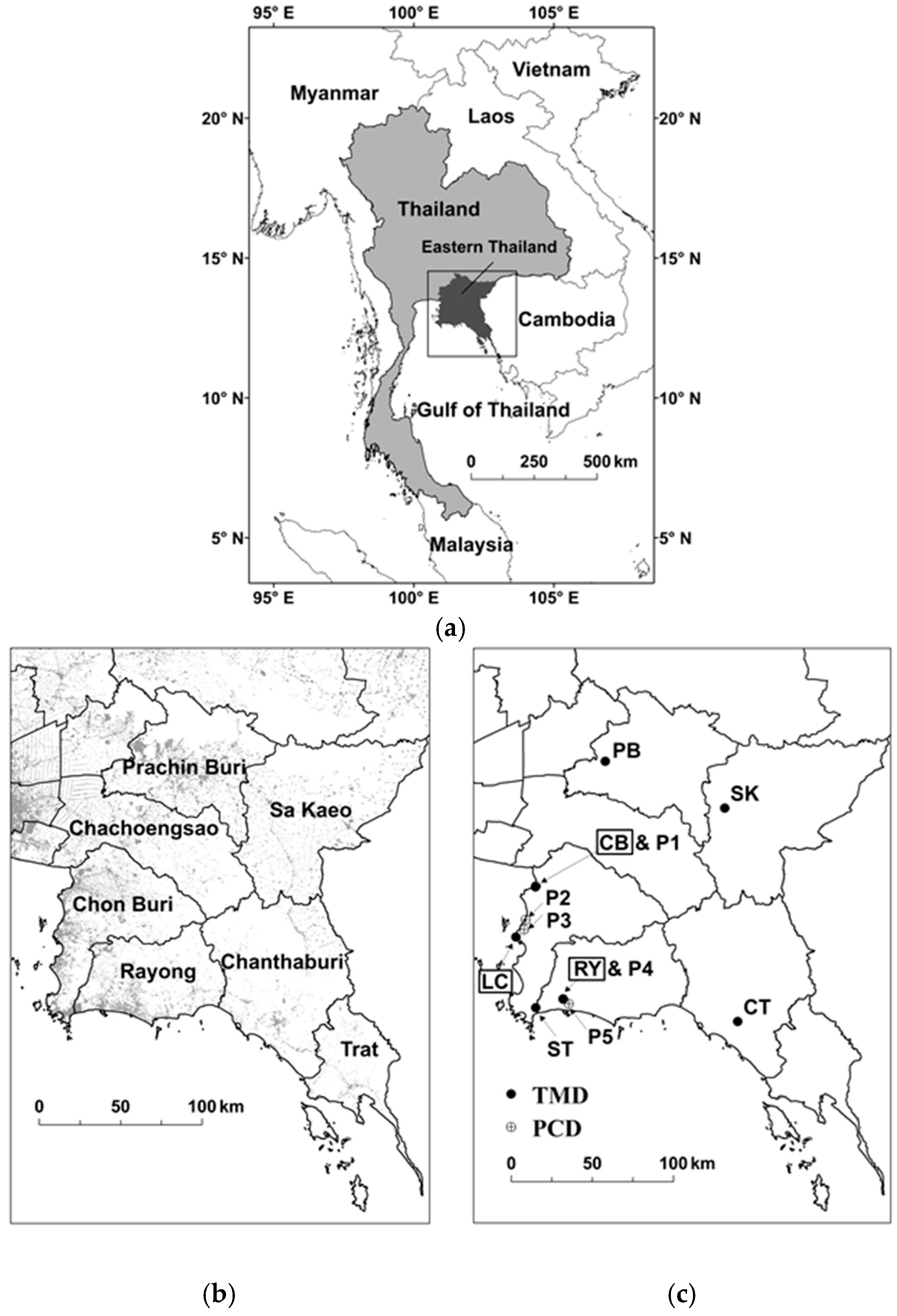
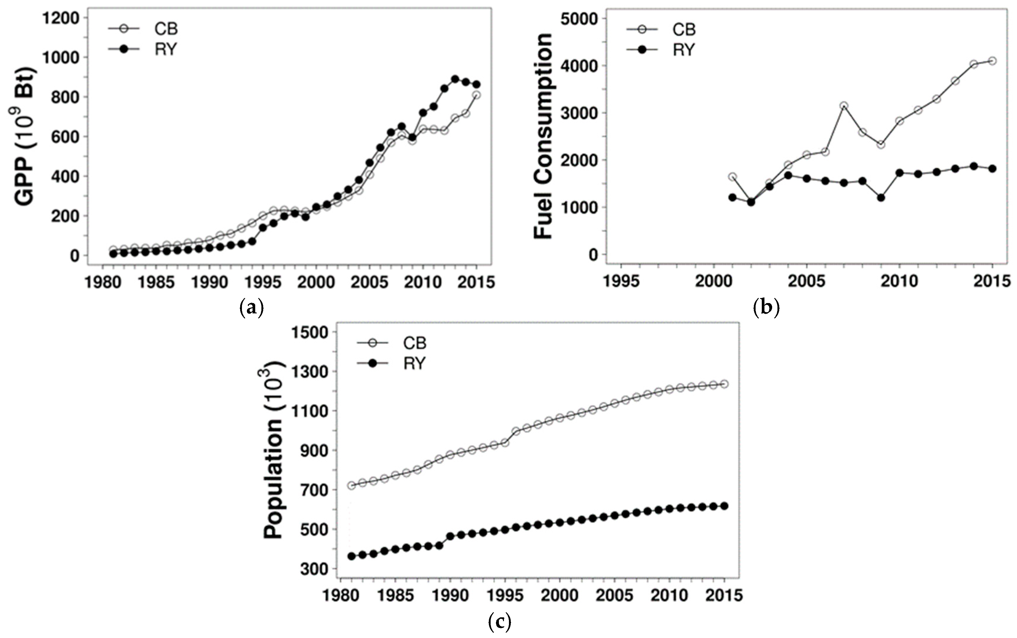
2.1. Study Area

The eastern region of Thailand has a total land area of 53,000 km² and is adjacent to the central region to the northwest, the Gulf of Thailand to the west (with a 100-km coastline) and to the south (with a 240-km coastline), the northeastern region to the north, and Cambodia to the west. Its topography is generally characterized by coastal plains and certain inland low mountains (<700 m above mean sea level) aligned in a north–south direction. Chon Buri and Rayong are the most developed provinces in the region, and are highly industrialized and fairly urbanized along their coasts (18% and 12% as built-up areas, respectively) based on Land Development Department (LDD) (2007) [34]. The two largest IEs in Thailand in terms of investment, Laem Chabang and Map Ta Phut, are also located in these two provinces, and are administered by the Industrial Estate Authority of Thailand (IEAT). The former IE is involved in manufacturing automobiles, electrical and electronic parts, engine machinery and spare parts, and steel/metal products, while the latter IE accommodates petrochemical, oil refinery, chemical and fertilizer, and steel/metal industries, as well as electricity generation.

The general climate of the eastern region is tropical humid and influenced by the northeast (November–February) and southwest (May–October) monsoons (as are most parts of the country, except for the peninsular southern region, which has a maritime-like climate) [35]. The northeast monsoon brings cool dry air from a persistent high-pressure system over continental mid-latitudes. The southwest monsoon causes the wet or rainy season since it carries moist air from the Indian Ocean and the Gulf of Thailand [35]. The transitional monsoonal period of March–April corresponds to the summer, with relatively high average temperature. Here, the winter and summer combined (i.e., November–April) is referred to as the dry season. Surface and synoptic winds in the atmospheric boundary layer generally follow the monsoons. Nevertheless, intense sea breezes can develop along the coasts due to a relatively large thermal land–sea contrast in the dry-season months, especially in January–March [36].

2.2. Data Collection and Treatment

In the initial step, meteorological data from all 15 available stations of the Thai Meteorological Department (TMD) and air quality data from six stations (located nearby these TMD stations) of the Pollution Control Department (PCD) located in the eastern region of Thailand were considered. The TMD data were requested from the agency directly and additionally compiled from the National Centers for Environmental Information (https://www.ncdc.noaa.gov/isd). Each of these stations has limited missing data for visibility (<10%). Given that human-observed visibility is based on a set of discrete targets (markers at different distances), inhomogeneity in visibility data can intrinsically arise when targets are changed or modified over time. However, no information of targets used in the past was available to us. Here, we proposed the use of a change point detection (CPD) technique [37,38] to identify such potential inhomogeneity due to changed or modified targets at each TMD station, and, if found, the station was removed. To conserve space, our CPD procedure is presented in Section S1 of the Supplementary Materials. A field visit to several TMD and PCD (see Appendix A for all symbols and acronyms) stations was conducted to evaluate monitoring conditions. Based on the CPD, visibility data from eight stations were not found suitable for use. Accordingly, air quality stations close to any removed TMD station were then removed at this stage. Finally, a total of seven TMD stations—CB (Chon Buri), LC (Laem Chabang), ST (Sattahip), RY (Rayong), CT (Chanthaburi), SK (Sa Kaeo), and PB (Prachin Buri)—and five PCD stations—P1 (General Education Office), P2 (Sri Racha Juvenile Center), P3 (Kasetsart University Sri Racha), P4 (Rayong Field Crops Research Center), and P5 (Map Ta Phut Health Center)—were finally selected (

Table 1. Monitoring stations and associated variables.

Station a	Agency	Province	Variables b	Period	Background c
CB	TMD	Chon Buri	VIS, RN, TEMP, RH, CC	1981–2015	Urban (coastal)
LC	TMD	Chon Buri	Same	2001–2015	Industrial (coastal)
ST	TMD	Chon Buri	Same	1981–2015	Suburban (coastal)
RY	TMD	Rayong	Same	2007–2015	Industrial (coastal)
CT	TMD	Chanthaburi	Same	1981–2015	Urban (coastal)
SK	TMD	Sa Kaeo	Same	2001–2015	Rural (inland)
PB	TMD	Prachin Buri	Same	1981–2015	Urban (inland)
P1	PCD	Chon Buri	PM10, SO2, NOx CO, NMHC, WS, WD	2001–2015	Urban (coastal)
P2	PCD	Chon Buri	PM10, NOx	2001–2015	Industrial (coastal)
P3	PCD	Chon Buri	PM10, SO2, NOx, CO, NMHC, WS, WD, GR	2001–2015	Industrial (coastal)
P4	PCD	Rayong	PM10, SO2, NOx, CO, NMHC, WS, WD, GR	2007–2015	Industrial (coastal)
P5	PCD	Rayong	PM10, SO2, NOx, CO, NMHC	2007–2015	Industrial (coastal)

^a CB: Chon Buri (WMO484590), LC: Laem Chabang (WMO484630), ST: Sattahip (WMO484770), RY: Rayong (WMO484790), CT: Chanthaburi (WMO484800), SK: Sa Kaeo (WMO484400), PB: Prachin Buri (WMO484300), P1 (General Education Office), P2 (Sri Racha Juvenile Center), P3 (Kasetsart University Sri Racha), P4 (Rayong Field Crops Research Center), and P5 (Map Ta Phut Health Center). Note that LC has only daytime monitoring from 0700 to 1900 LT. It is noted that P2 has been slightly relocated to a nearby site (<100 m away) since September 2013; however, it is still in the same background as its original site. ^b VIS: Visibility; RN: Rain; TEMP: Air temperature; RH: Relative humidity; CC: Cloud Cover; PM₁₀: Particulate matter with size smaller than or equal to 10 µm; SO₂: Sulphur dioxide; NO_x: Nitrogen oxides; CO: Carbon monoxide; NMHC: Non-methane hydrocarbon; WS and WD: 10-m wind speed and direction, respectively; and GR: Global radiation. Thai Meteorological Department (TMD) data are three-hourly while Pollution Control Department (PCD) data are hourly. ^c Background of each visibility station: (a) CB has a dense urban background. It is located close to the coast (0.8 km to the west) and near highways nos. 3 and 7 (0.25 km and 6 km to the east, respectively), with an Industrial Estate (IE) 15 km to the northeast. (b) LC has an industrial background. It is next to the coast (to the west) and Laem Chabang Seaport (to the south) and separated from the two highways by 5 km and 13 km to the east, respectively. It is also close to the Laem Chabang IE (3 km to the east). (c) ST has a suburban background. It is close to highway no. 3 (0.5 km to the north) and the U-Tapao International Airport (2 km to the west). RY has an industrial background. It is close to highway no. 3 and the Map Ta Phut industrial complex (0.1 km and 3 km to the south, respectively). (d) CT is in a non-dense urban area near highway no. 3 (3 km to the east) and not far from the coast (16 km). (e) SK is in a rural area and near highway no. 33 (5 km to the north). (f) PB is in a non-dense urban area, located next to a major river and near highway no. 33 (8 km to the north).

and Figure 1c). The temporal coverage of visibility data at the selected stations spans 1981–2015 (35 years) for four stations, 2001–2015 (15 years) for two stations, and 2007–2015 (nine years) for one station (Table 1). We placed emphasis on the three stations located in the developed coastal areas: CB (urban background), LC (industrial), and RY (industrial). Each of these stations has one or two PCD stations located nearby, feasibly allowing visibility and air quality data to be paired together for the analysis. Here, CB, LC, and RY were paired with P1, P2 and P3, and P4 and P5, respectively. The TMD data have a three-hourly resolution, reported at 0100, 0400, 0700, …, 1900, and 2200 local time (LT), and include visibility (VIS), air temperature (TEMP), relative humidity (RH), cloud cover (CC), rain (RN), and weather code (e.g., fog, haze, and smoke occurrence). The PCD data have an hourly resolution and include measurements of PM₁₀, sulfur dioxide (SO₂), nitrogen oxides (as the sum of nitrogen oxide and nitrogen dioxide, i.e., NO_x = NO + NO₂), carbon monoxide (CO), non-methane hydrocarbons (NMHC), 10-m wind (WS: wind speed; and WD: wind direction), and global radiation (GR). All data are from near-surface monitoring, except for winds at about 10 m above ground level (AGL). It is noted that wind data at the selected TMD stations have the potential to be strongly affected by nearby objects or infrastructure. Thus, PCD wind data were used. Data completeness, unit consistency, and data ranges of the meteorological variables were examined based on the WMO guidelines [39]. Any improbable or spurious values were converted to missing. In addition to the conventional meteorological variables, recirculation factor (RC) and mixing height (MH) were also derived. As noted in Section 2.1, sea breeze is very present in the dry season during the daytime hours along the coasts in the region in question, potentially suppressing the ventilation of air pollutants out of the coastal areas due to horizontal wind circulation. The RC aims to account for this local effect during daytime hours (here, 1000–1800 LT), and is computed as follows [40]:

$$RC=1-\frac{\sqrt{X^2+Y^2}}{WR},$$

(1)

where WR is the total wind run or summed distance by an air mass over a period of time, and X and Y are the total distances travelled by the air mass in the east–west and north–south directions, respectively. In other words, $WR=T{{\displaystyle \sum }}_{i=1}^N\sqrt{u_i^2+v_i^2}$, $X=T{{\displaystyle \sum }}_{i=1}^N{u}_i$, $Y=T{{\displaystyle \sum }}_{i=1}^N{v}_i$, where u_i and v_i are the x-axis and y-axis wind components, respectively, N is the total hours of air-mass migration (here, 1000–1800 LT as the daytime hours), and T is the time interval (here, one hour). Mixing height determines the degree of atmospheric dilution. Here, mixing height was computed using AERMET (American Meteorological Society/Environmental Protection Agency Regulatory Model Meteorological Processor), the meteorological preprocessor for the AERMOD (American Meteorological Society/Environmental Protection Agency Regulatory Model) dispersion modelling system developed by the US EPA (US Environmental Protection Agency) [41], which is based on a one-dimensional heat balance in the atmospheric boundary layer. The required input to AERMET includes both radiosonde sounding and surface variables. As no radiosonde sounding is routinely conducted by the TMD in the eastern region of Thailand, reanalysis data were adopted for substitution, as in Assareh et al. (2016) [18] and Chusai et al. (2012) [19]. Climate Forecast System Reanalysis (CFSR) data [40] were chosen given their moderate grid resolution (0.5°). Running AERMET additionally requires long-term historical rainfall data for surface wetness characterization, and we here obtained and used TMD daily rainfall data from the past 35 years (1981–2015). The details of the AERMET setup and its input preparation are presented in the US EPA (2004) [41].

Daily daytime visibility (daily visibility) is of interest to us, and was here defined as the minimum of the visibility values at 1300 and 1600 LT. The reasons for choosing the daytime visibility are that: (1) using a single (or a few) observation(s) per day, rather than taking an average, automatically reduces the change in targets’ light illumination with time; and (2) using only afternoon hours avoids the effects of lower solar elevation and diurnal change of meteorological factors over the course of the day [6,42]. With these, diurnal characteristics are not our focal point; however, they are concisely described in the Supplementary Materials (see Figure S1). To assign daily values to other variables, those corresponding to the times at which daily visibility was chosen were used. As for data completeness, the amount of missing data (in terms of available daily visibility) at every station was found to be small (<4% and <1% in the dry and wet seasons, respectively) (Supplementary Materials, Table S1).

Certain meteorological conditions (humid air, rain, fog, and mist) have the potential to reduce visibility and are thus not relevant when attention is given to visibility reduction by anthropogenic activities. Accordingly, meteorological screening was applied, in which data are excluded when rainfall, mist, fog, or very moist conditions (RH > 90%) are present, similar to other studies [5,10,43], highlighting the anthropogenic influence on visibility. This exclusion will hereafter be referred to as “met-screening”. In general, moderate-to-high relative humidity can effectively impact visibility since most atmospheric aerosols can absorb humidity (i.e., are hygroscopic) and then grow in size, which in turn increases light scattering efficiency and lowers mean refractive index, reducing visibility [1]. To adjust or correct original visibility to the non-humid (or dry) condition (corrected for hygroscopic effect of aerosols), the following relationship was applied [44]:

$$\frac{VIS}{VI{S}_{\mathrm{d}}}=0.26+0.4285{\log }_{10}\left(100-RH\right),$$

(2)

where VIS_d is the RH-corrected visibility. For RH <40%, the effect of humidity is only small and the above adjustment is not required. After the met screening, the number of excluded days found in the dry season ranged between 4 and 24% (of total days in the dry season) among the TMD stations, with higher values seen at the coastal stations which tend to have humid or wet conditions more often than those inland. In the wet season, the exclusion is higher (21–60%) as expected (Supplementary Materials, Table S1).

2.3. Monthly Variation, Seasonality and Relation with PM₁₀

In order to understand seasonality, we here simply defined the seasonality index (SI) for visibility as the difference between the two seasonal averages, normalized by the dry-season average, i.e.,:

$$SI (\%)=\left(\frac{{\overline{VIS}}_{\mathrm{wet}}-{\overline{VIS}}_{\mathrm{dry}}}{{\overline{VIS}}_{\mathrm{dry}}}\right)\times 100.$$

(3)

The seasonality index for visibility was calculated for both met-screened visibility data and original visibility data. Additionally, we calculated the monthly average for visibility and other meteorological variables based on daily data. The understanding of seasonality and monthly variation helped us determine that visibility degradation is mainly a problem in the dry season (discussed in Section 3.1) and hence was chosen for this study.

The relationship between visibility and PM₁₀, was analyzed in three ways: (a) correlation analysis; (b) mean PM₁₀ under different visibility classes; and (c) weekday and weekend differences. Visibility classes (e.g., poor and good) have often been used in visibility assessment [14,45], offering convenience in public communication and also partially reducing the effect of changed visibility targets. As suggested by the US EPA (1987) [43], visibility classes were selected based on yearly frequency, with the lowest upper limit (of visibility target) found over a period of time used as the best visibility class and the remaining classes based qualitatively on their frequency and separation. This procedure facilitates a set of common visibility classes for all stations, although with different thresholds. In this study, three classes were defined: I (good), II (moderate), and III (poor). The thresholds separating Classes I and II and Classes II and III were respectively assigned as follows: (a) Visibility of 14 km and 6 km for CB, RY, and ST; and (b) Visibility of 12 km and 6 km for the other stations. The prevalence of good-, moderate-, and poor-visibility days are reasonably reflected before and after the met-screening at every TMD station (Supplementary Materials, Figure S2). Accordingly, we considered these thresholds acceptable for use. How visibility differs during the weekdays and the weekend has an implication on anthropogenic influence and is addressed here. It is a general assumption that human activities tend to intensify during the weekdays and reduce over the weekend. Here, Sunday, along with national holidays, local holidays, and atypical days (e.g., those with political protest) were treated as “weekend days” while the remaining days were treated as “weekdays”. The weekdays share 80% of all dry-season days. Saturday was not included in the weekend as large urban and industrial areas in Thailand are generally busy or operating like on Monday–Friday, which is likely to be the case in Chon Buri and Rayong provinces where businesses and factories are run on Saturday, having relatively large emissions of air pollutants. However, the industrial and power plant sectors in Thailand have reduced total workloads and emissions on Sunday [30].

2.4. Equal Step-Size Method for Visibility and Relative Humidity Relationship

Not does RH affect the source and sink of the aerosol particles but also the size, structure and composition of aerosol particles [1,46]. The effect of RH on visibility can be separated as two physical processes [47,48,49]: (a) hygroscopic growth of aerosol particles and (b) change in the mass concentration of aerosols and the size distribution of dry particles. Here, an equal step-size statistical method was employed to understand the relation between visibility and RH [6,47]. The RH data was divided into 11 intervals: 0–40%, 40–45%, 45–50%, 50–55%, 55–60%, 60–65%, 65–70%, 70–75%, 75–80%, 80–85%, and 85–90%. The setting of the first interval (0–40%) was based on Equation (2) as the hygroscopic effect being very low or negligible when RH < 40%. Average visibility, RH-corrected visibility, and PM₁₀ were calculated for each interval. The difference between visibility and RH-corrected visibility with varying RH partly relate to the relative dominance of the two physical processes.

2.5. Polar Plot for Visibility and Back Trajectory Modelling

Next, the effects of local wind and long-range transport on visibility degradation were investigated. Wind advection carries air masses to a receptor area or site. They can absorb airborne constituents emitted from or existing at places/areas during migration. Such constituents can be either clean or polluting, and either dry or moist. The long-range transport of airborne constituents is known as a physical mechanism at a regional scale, which can potentially impact local conditions. In view of visibility, moisture and air pollutants can be absorbed and carried along in air masses moving through areas before reaching a receptor. The effect of local wind on visibility degradation has been analyzed using polar plots [50] looking at the climatological patterns of visibility as a function of local wind speed and direction for the three main stations. For analyzing the effect of long-range transport, we performed back-trajectory modeling, which is a useful tool to examine such impacts [51,52]. Here, daily kinematic trajectories were generated using FLEXTRA (version 5) (http://flexpart.eu) [53] and driven by the six-hourly 0.5°-resolution wind fields of the CFSR data [54]. Each back trajectory that represents a daily air mass was tracked backward in time for five days for the dry season. The latitude, longitude, and height of the air mass were recorded along its migration. The arrival time was 1300 LT when mixing height was generally well developed and well mixed throughout the atmospheric boundary layer. The arrival height was set as 500 m AGL, approximately the middle of the atmospheric boundary layer. A conventional K-means clustering method was used to divide all finally obtained back-trajectories into clusters. The objective of the K-means method is to minimize the sum of the square of Euclidean distance of within-cluster members from their center [55]. Here, the K-means clustering was carried out in the R computing environment [56], in which scree and silhouette diagrams were employed to guide the optimal number of clusters. Since stations CB and LC are in the same province and the distance between them is not far (33 km) compared to the CFSR grid spacing, the back-trajectory modeling was performed only at CB and RY.

2.6. Potential Role of Secondary Aerosols

A precursor-ratio method used by Quan et al. (2014) [13] and Zhang and Cao (2015) [57] was adopted to ascertain the potential influence of secondary aerosol formation on visibility, using the precursors of secondary aerosols as a proxy for secondary aerosol formation. SO₂, NO_x, and volatile organic compounds (VOCs) are among the major precursors of secondary aerosols formed in the troposphere. CO is generally emitted from incomplete combustion by various primary sources. It has a relatively long chemical lifetime compared to other typical air pollutants, and can therefore be used as tracer for primary emissions. By computing the ratios of PM₁₀, SO₂, NO_x, and NMHC (for VOCs) to CO under different visibility classes, one may expect more secondary aerosols produced to be coupled with larger PM₁₀/CO but lower SO₂/CO, NO_x/CO, and NMHC/CO. That is, SO₂, NO_x, and NMHC loss is assumed to be converted to sulfate, nitrate, and secondary organic aerosols, respectively. Daily average concentrations for different pollutants were used for analysis here, and were decided based on the diurnal variation of these pollutants.

2.7. Long-Term Trends and Meteorological Adjustment

In the following, trends in dry-season average visibility at all seven TMD stations (CB, LC, RY, ST, CT, SK, and PB) were estimated using linear regression. A non-parametric Mann–Kendall test was employed in conjunction with block bootstrapping (to account for serial correlation in a time series) to test the significance of trend (against the null hypothesis of no trend) [58]. At CB, ST, CT, and PB, long-term data (since 1981) are available; it was then possible to perform trend estimation over two consecutive periods: P1: pre-2000 (1981–2000); and P2: post-2001 (2001–2015). For LC, SK, and RY, the trend analysis was limited to the recent period (starting with the years 2001, 2001, and 2007, respectively) only.

In order to account for the effect of meteorology on trends in visibility, a generalized linear model (GLM) framework, used by Camalier et al. (2007) [59], was adopted. GLM is an advanced statistical model capable of accounting for relationship between response (i.e., predictand) and explanatory (i.e., predictor) variables via a link function [60,61]. Visibility at each of the CB, LC, and RY stations is the interested response variable, while meteorological variables are the predictors, whose GLM formulation is given by:

$$g\left({\mu }_i\right)~f_1\left(x_{i,1}\right)+f_2\left(x_{i,2}\right)+\dots f_j\left(x_{i,j}\right)+\dots +f_p\left(x_{i,p}\right)+Y_k,$$

(4)

where subscript i denotes the ith observation and subscript j (1, 2, 3, …, p) denotes the jth predictor variable, $f_j\left(x_{i,j}\right)$ is the smoothing function (here cubic spline) of the jth predictor at the ith observation, ${\mu }_i$ is the ith value of the response variable, $Y_k$ is the effect of the kth calendar year, and $g\left({\mu }_i\right)$ is the link function relating the mean of the response variable to the predictors. Here, GLM was implemented in the R software [56]. Several options of error distribution and link function were tried, and Gaussian distribution and identity link were finally chosen since they tend to give an optimal fit. The adjusted coefficient of determination (shortly, adjusted R²), representing variance of data explained (%) by the model, was used as the goodness-of-fit measure for each GLM model. Residual diagnostics (here, independent error, normality of error, homoscedasticity of error, and outlier leverage) were inspected and found to be fairly acceptable [55]. A parsimonious approach was adopted to achieve the final model. Eight predictors were initially chosen for the GLM, namely temperature, relative humidity, cloud cover, mixing height, wind speed, recirculation factor, back-trajectory cluster, and persistence (Supplementary Materials, Table S2). Persistence was here assigned as the daily value from the previous day and included to represent inter-day impact or imprint generally due to atmospheric stagnation or lack of atmospheric ventilation. It is noted that certain variables were not included in this initial list due to their correlation with one of the initial variables, e.g., global radiation and cloud cover. Similarly, the entire GLM procedure was applied to PM₁₀ but with log transformation. Given Equation (2), relative humidity with and without log transformation was tried but gave comparable results in both visibility and PM₁₀ cases. Thus, no log transformation was used here. In the GLM processing, stepwise backward elimination was carried out to obtain a parsimonious fit. Given the final GLM fit achieved, a meteorologically adjusted trend (adjusted trend) was computed from the partial response with respect to the effect of the calendar year ($Y_k$).

3. Results and Discussion

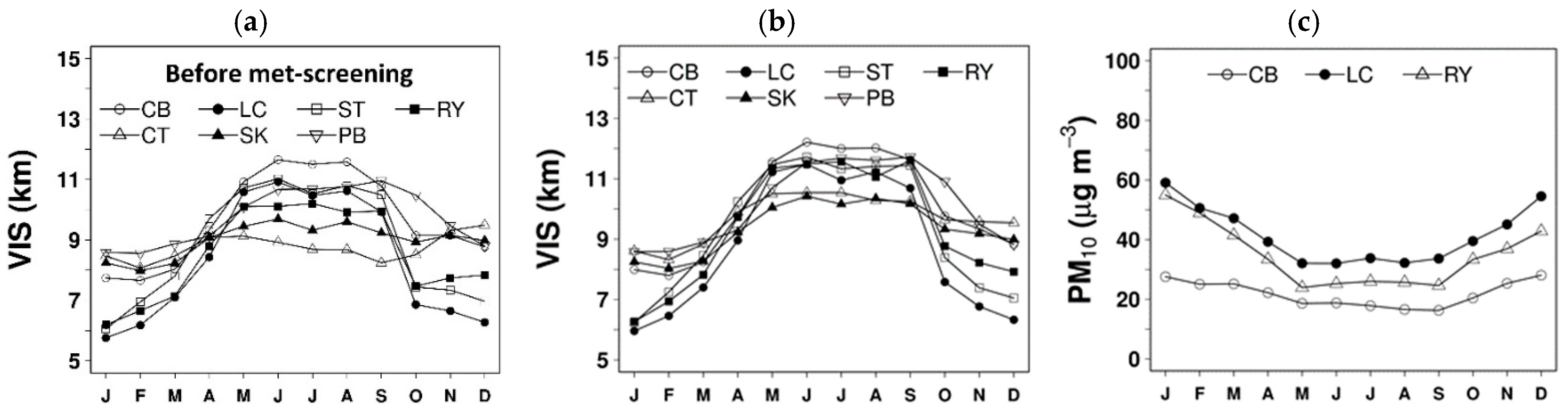
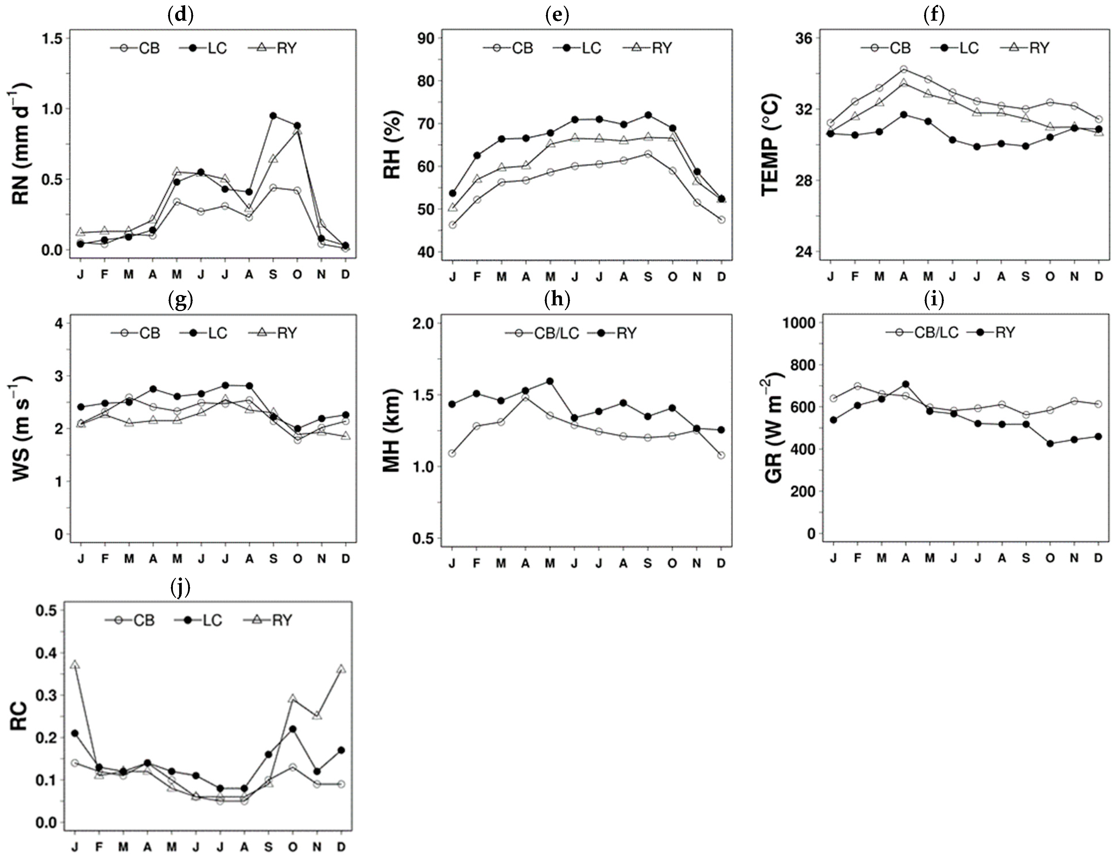
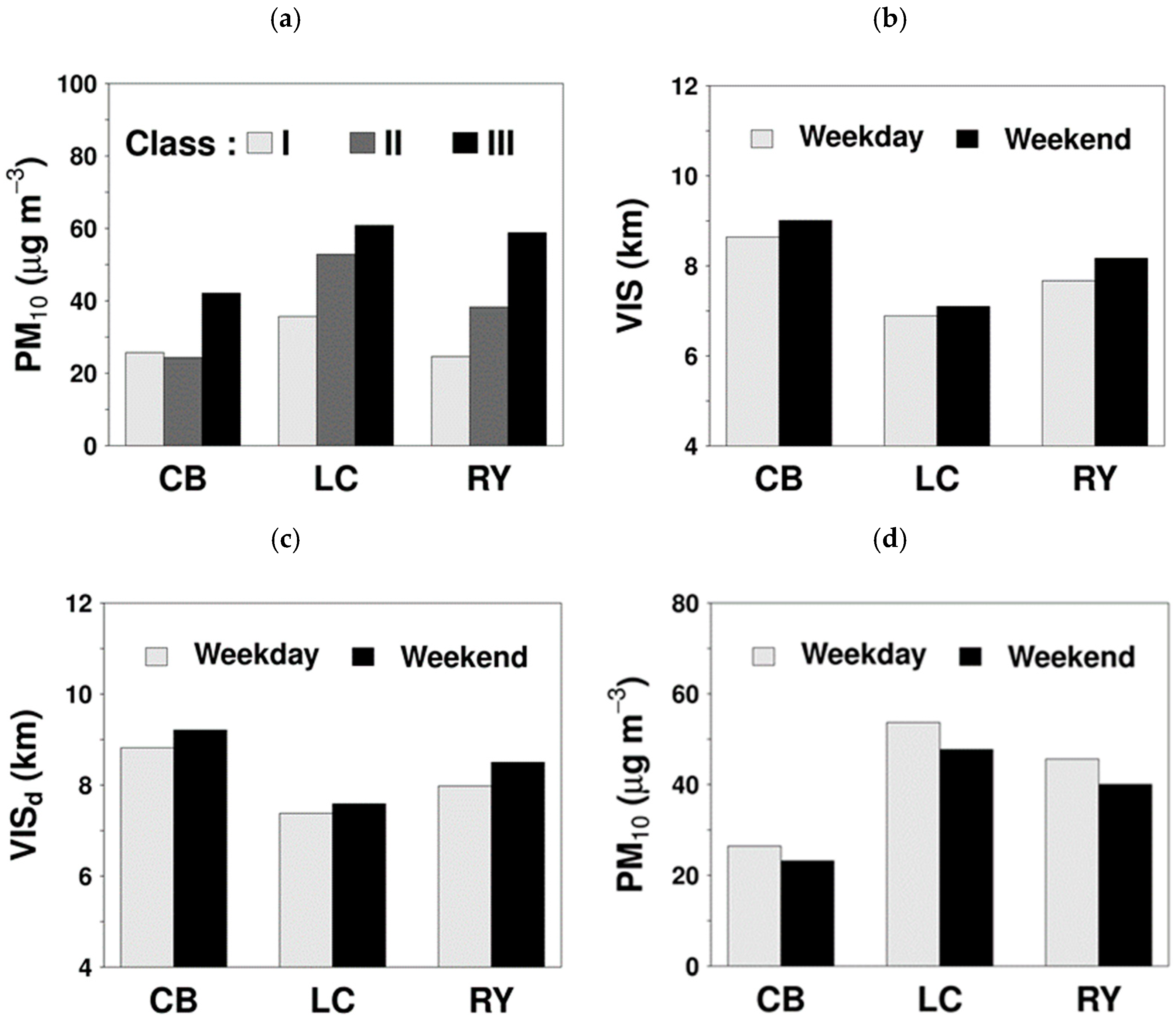
3.1. Monthly Variation and Seasonality

Before the met screening, every station had an SI close to 10% or larger, except for CT (−1.2%) (Supplementary Materials, Table S3). After the met screening, these improved to 19% for CT and the SI range among all stations was 16–55%. Visibility varies over the months of the year at every TMD station, as do the other variables at CB, LC, and RY (Figure 3). They demonstrate a contrast between the dry and wet seasons (i.e., seasonality). Visibility tends to be high in the wet season but lowers in the dry season at most stations (five out of seven) due to effective wet scavenging by monsoonal rain (Figure 3a,d), as seen from the monthly PM₁₀ values in Figure 3c. At CT and SK, seasonality is not initially apparent, but is much clearer after the met-screening (Figure 3b). In relative terms, rain and humidity are high in the wet season due to the southwest monsoon, and vice versa in the dry season. Temperature is straightforward, being low, high, and mild in the winter, summer, and wet season, respectively. Winds are strong in the wet season given their location facing the southwest monsoonal winds. In October, wind speed becomes the lowest as the southwest monsoon weakens and comes to an end, however it increases once the northeast monsoon starts to prevail. The northeast monsoon is continental and can absorb and transport polluted air from distant areas before reaching the stations (as opposed to the southwest monsoon, which is generally maritime and clean). Mixing height is low during December–January due to cool weather and frequent atmospheric subsidence induced by the high-pressure system responsible for the northeast monsoon during those two months, however it increases during March–May due to warm conditions and a lack of strong subsidence. March and April are the warmest months and also mark the time at which the northeast monsoon is weak and then comes to an end. Solar radiation is strong over most of the dry season but decreases in the wet season, generally due to cloud and rains. The recirculation factor is large in the dry season, due partly to frequent sea breeze occurrences [36]. The combination of many of these factors (such as low wet scavenging, low mixing height, large recirculation factor, and long-range transport) can contribute to visibility reduction in the dry season.

3.2. Visibility in Relation to PM₁₀

The association between visibility and PM₁₀ is generally acknowledged. Here, visibility was also found to be negatively correlated with PM₁₀, with correlation coefficients of −0.29 (on the daily data) and −0.22 (on the monthly data) at CB, −0.32 (daily) and −0.23 (monthly) at LC, and −0.51 (daily) and −0.64 (monthly) at RY. The correlation coefficient values using RH-corrected visibility do not differ much (only by 1–2% in magnitude for all cases). Such negative association between visibility and PM₁₀ is also manifested in mean levels of PM₁₀ under different visibility classes (Figure 4a). That is, Class III has an average PM₁₀ concentration of 42–60 μg m⁻³, which is about 1.6–1.7 times higher than that in Class I. It was found that average visibility is significantly higher over the weekend (9.1 km, 7.1 km and 8.2 km for CB, LC and RY, respectively) than on weekdays (8.6 km, 6.8 km, 7.6 km) which can be explained with significant lower mean level of PM₁₀ during weekend at the three stations (Figure 4b–d). A non-parametric Wilcoxon rank sum test (at a significance level of 0.05) was employed here to inspect the statistical significance of the mean (i.e., average) difference between two samples. It is noticed that the patterns of weekday–weekend difference are similar for both visibility and RH-corrected visibility due to the lack of significant difference in relative humidity (on average) between the two periods (not shown). The above results provide evidence of anthropogenic influence (here, in view of PM₁₀) on visibility.

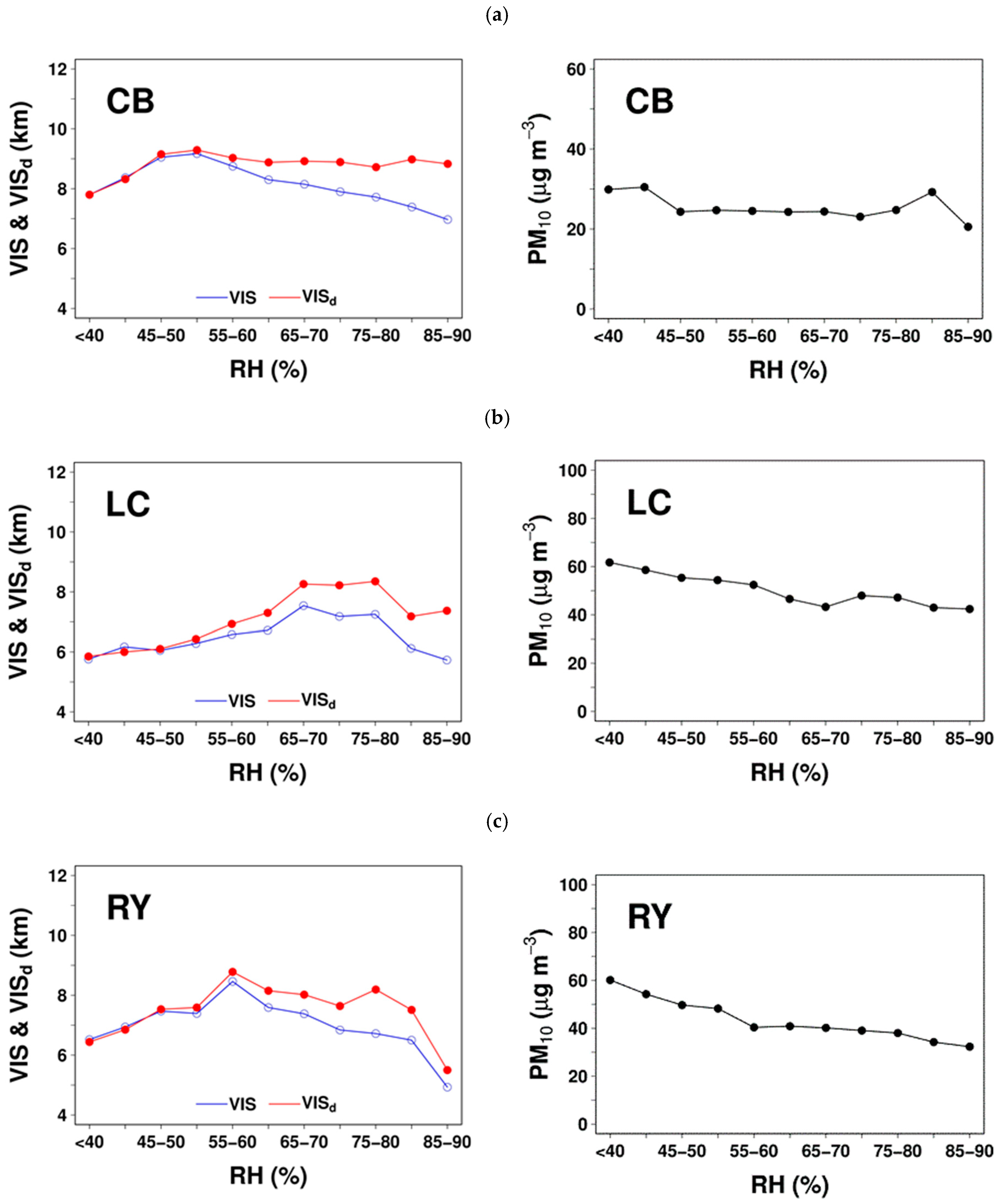
3.3. Visibility in Relation to Relative Humidity

All the three stations show similar patterns with regards to change in visibility with RH. Visibility initially increases with RH but begins to decrease once a threshold RH interval is reached, which is approximately 50–55% at CB, 65–70% at LC, and 55–60% at RY respectively (Figure 5). The results shows negative effect of RH on visibility. Over low RH intervals, visibility and RH-corrected visibility (corrected for hygroscopic growth) do not show much difference, suggesting no or limited hygroscopic effect as compared to change in size distribution of dry particles. As RH increases, the hygroscopic effect becomes the dominating process as seen with the increasing difference in visibility and RH-corrected visibility. Change in mean level of PM₁₀ under different RH intervals shows the contrasting results (Figure 5). PM₁₀ does not show any change with RH over CB while it decreases over LC and RY. This decrease in visibility with increase in RH in spite of either no change or decrease in PM₁₀ clearly indicates the effect of hygroscopic growth of aerosols on visibility. However, it should also be noted that the effect of RH on aerosols is sensitive to aerosols size distribution and chemical constituents [1,47]. Mass concentration and chemical constituents of aerosols of difference size ranges under different RH intervals will give better understanding of effect of aerosol characteristics on visibility relation with RH, which is not available for this study.

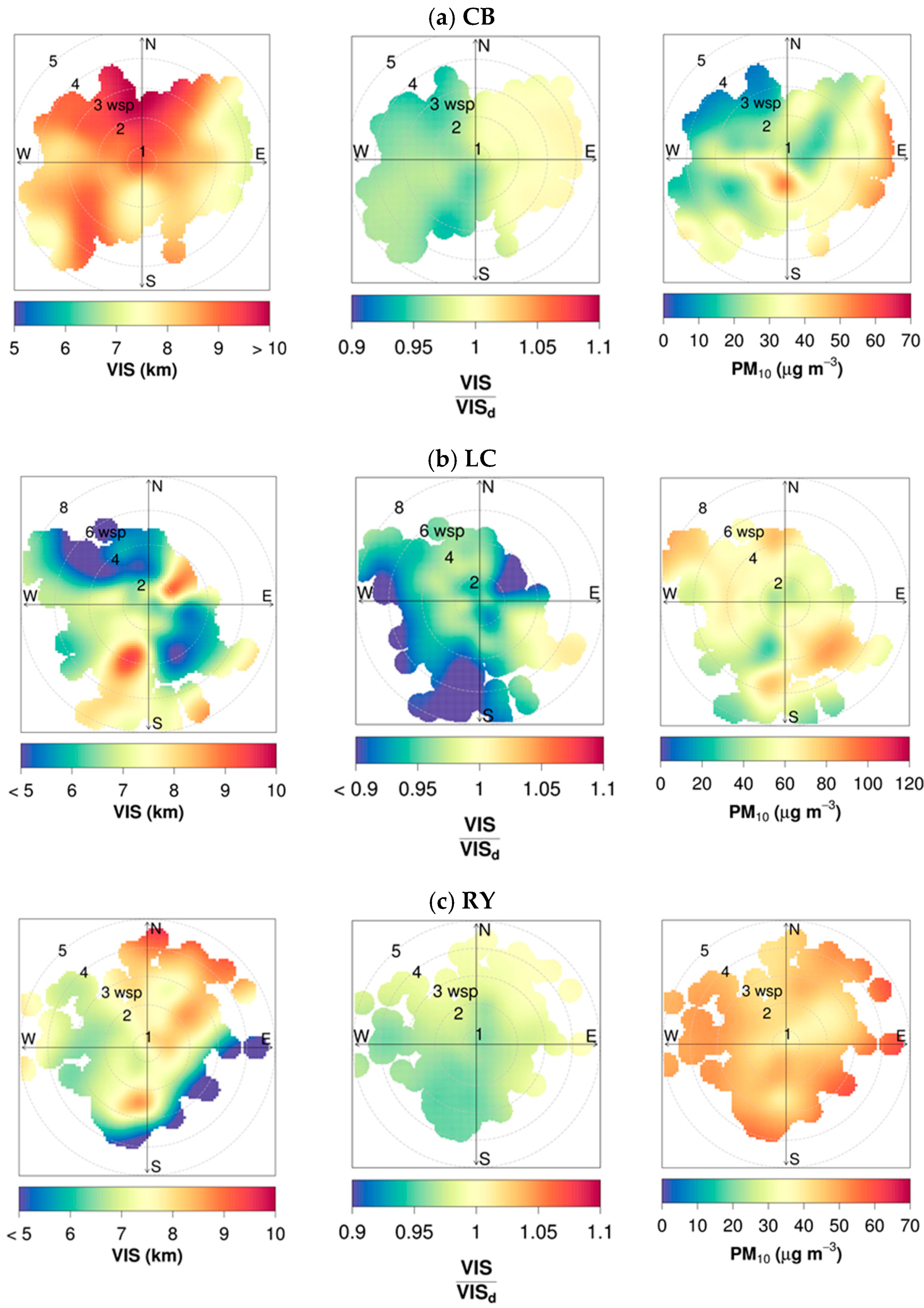
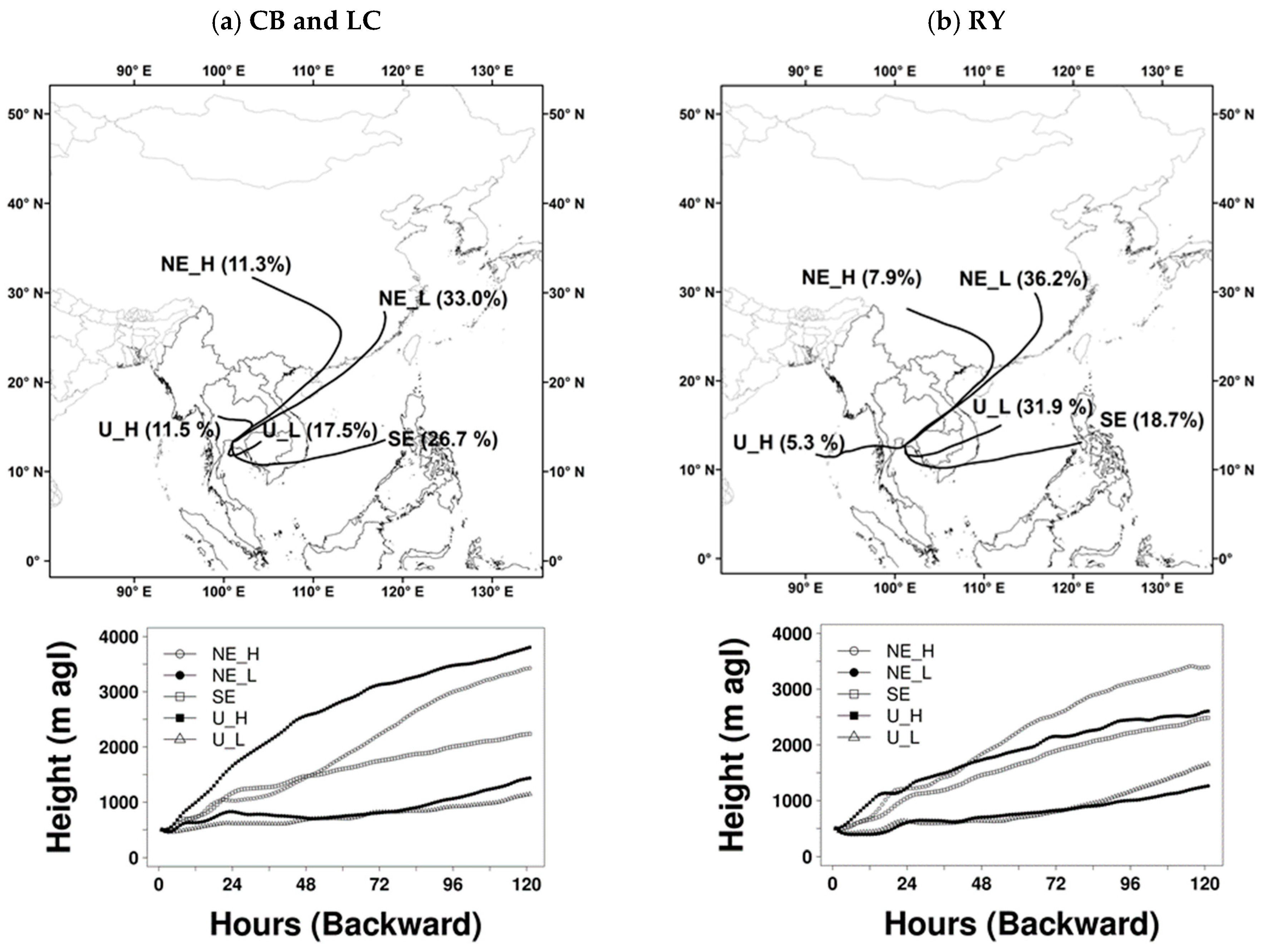
3.4. Effect of Local Wind and Long Range Transport

The dependency of visibility on local wind direction can be seen in both stations CB and LC. At CB (Figure 6a), relatively low visibility and high levels of PM₁₀ are seen in the northeastern, eastern, and southern directions, which is attributable to the advection of pollutants from the nearby industrial sources and highways (Table 1, and Figure S3 in Supplementary Materials). By contrast, relatively good visibility is mostly seen in the north given the fewer emission sources present upstream of the station. However, in the southwest and the west, visibility appears to be moderated by moisture from the sea, as seen from the VIS/VIS_d ratio being smaller than unity (here, 0.95). At LC (Figure 6b), visibility tends to be lower than CB, in general agreement with the higher level of PM₁₀. Poor visibility (5–6 km or less) is noticeable in the southeast direction due mainly to the presence of industries and highways. However, poor visibility is even more pronounced in the northwest due potentially to the combination of moisture and air pollutants generated from intense shipping activities in and around this coastal area. At RY (Figure 6c), both visibility and PM₁₀ levels appear to have lesser directional dependence, possibly because of the station having industrial facilities and highways nearby in various directions (Table 1, and Figure S3 in Supplementary Materials). The visibility reduction is most intensified from the east to the south given that moisture and emission sources tend to align in those directions.

Back-trajectory modelling shows a total of five similar clusters at both stations: (1) northeasterly and high level (“NE_H”) (with occurrences of 11.3% of total days at CB and 7.9% at RY); (2) northeasterly but low level (“NE_L”) (33% at CB and 36.2% at RY); (3) southeasterly (“SE”) (26.7% at CB and 18.7% at RY); (4) undefined and high level (“U_H”) (11.5% at CB and 5.3% at RY); and (5) undefined and low level (“U_L”) (17.5% at CB and 31.9% at RY) (Figure 7).

Table 2. Average visibility, RH, RH-corrected visibility, and PM₁₀ by back-trajectory cluster at stations CB, LC, and RY.

Station	% of Days	VIS (km)	RH (%)	VISd (km)	PM10 (μg m−3)
CB
NE_H	11.3	8.5	45.5	8.6	29.0
NE_L	33.0	8.8	47.8	8.9	25.9
SE	26.7	8.6	56.7	9.0	23.8
U_H	11.5	8.5	46.9	8.6	25.4
U_L	17.5	8.9	57.8	9.4	26.2
LC
NE_H	11.3	6.1	48.8	6.2	57.6
NE_L	33.0	6.3	53.1	6.5	53.7
SE	26.7	8.1	66.9	8.9	50.9
U_H	11.5	6.4	52.3	6.6	57.3
U_L	17.5	7.5	65.8	8.2	49.5
RY
NE_H	7.9	7.3	53.4	7.6	45.0
NE_L	36.2	7.4	53.2	7.6	46.7
SE	18.7	7.7	58.1	8.1	42.5
U_H	5.3	9.4	59.3	9.8	29.4
U_L	31.9	7.9	55.4	8.2	44.1

summarizes cluster-average visibility, RH, RH-corrected visibility, and PM₁₀. Using the Wilcoxon rank sum test (at a 0.05 level), most of the cluster pairs (>50%) were found to have significant difference in average visibility and average PM₁₀. In relative terms, low visibility generally occurs in the northeasterly clusters, as seen in NE_H at CB (8.5 km) and NE_H and NE_L at both LC (6.1 and 6.3 km) and RY (7.3 and 7.4 km). A similar pattern was also seen for RH-corrected visibility. The northeasterly clusters represent continental air masses and tend to be more polluted and less moist. Thus, it is possible to say that such low visibility is mainly influenced by pollution, causing relatively high PM₁₀ in these two clusters. In the dry season, biomass burning (forest and agricultural fires) is typically intensified over certain areas of the Indochinese Peninsula (e.g., Northern Thailand, Northern Laos, and Eastern Myanmar) and part of Southern China during March–April. Based on satellite fire hotspot data [62], many trajectories of these two clusters pass such fire-prone areas that could contribute smoke and other pollutants to the migrating air masses (not shown). The SE cluster tends to have high humidity since it is semi-maritime with many trajectories originating from and/or passing the sea (not shown), with its associated visibility, RH-corrected visibility, and PM₁₀ rank between the best and the third across the stations. For U_H and U_L, their migrations are relatively short and then have a long residential time to stay within or around the region. As a result, the effects of pollution and humidity may be confounded and not readily discerned. Nevertheless, at RY, U_H is regarded as maritime and clean with the highest visibility and the lowest PM₁₀ across the clusters.

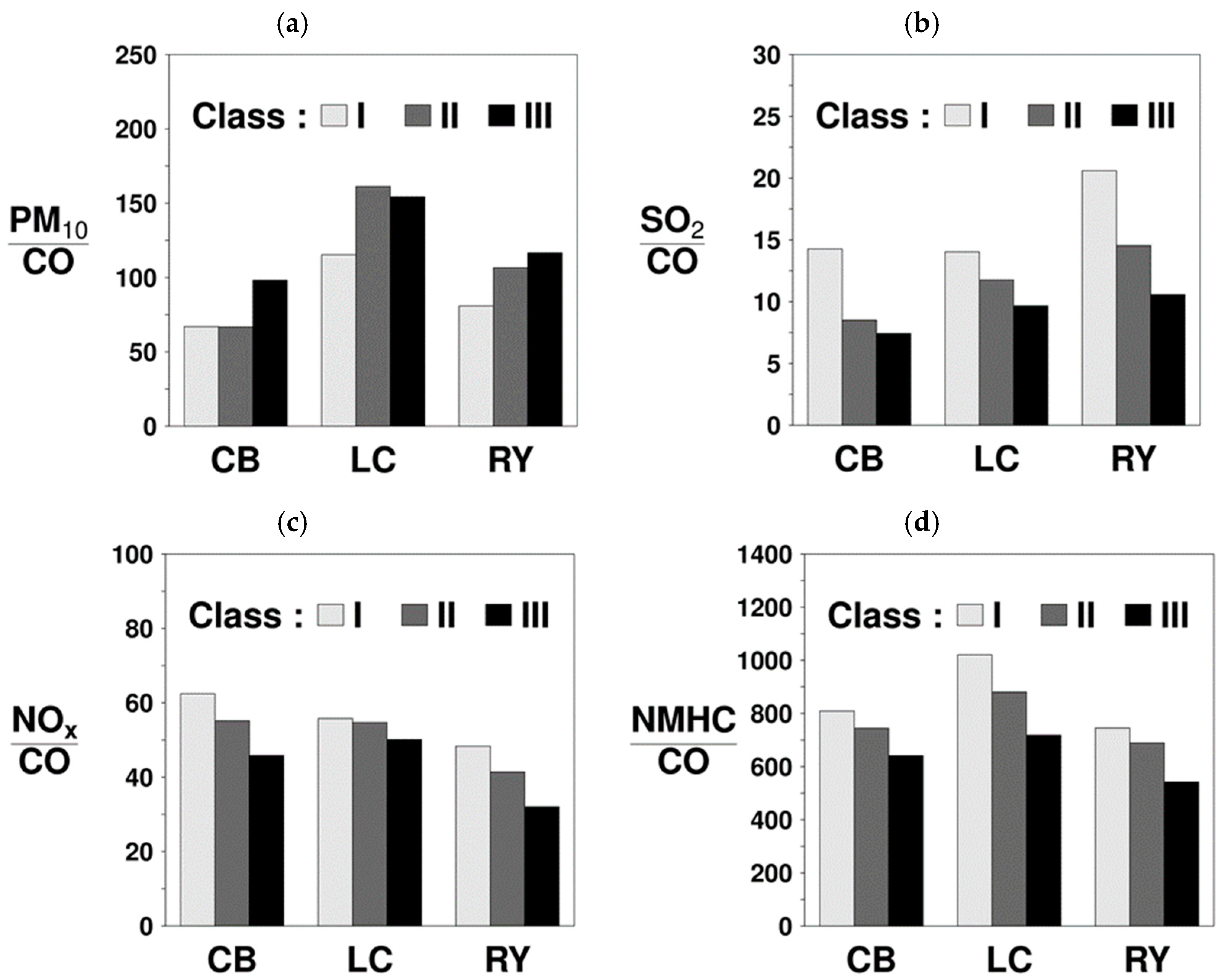
3.5. Effect of Secondary Aerosols on Visibility

Based on the diurnal variation of PM₁₀, NO_x, SO₂, NMHC, and CO levels, their average concentration over 0600–1600 LT were computed to convert to daily data. These selected daytime hours include the early morning, when pollutants can reasonably be assumed to represent fresh anthropogenic emissions (e.g., from rush-hour activities), and the later hours when complex photochemical reactions evolve. This is generally the time when most of the pollutants tend to concentrate with relatively low mixing height (Supplementary Materials, Figures S1 and S4). It is noted that the peak in SO₂ level occurs in the afternoon at LC and RY but in the early morning and evening at CB. Xu et al. (2014) [63] also reported such afternoon peaks of SO₂ in the North China Plain and suggested several possible causes: down-mixing of pollutant layers aloft, plume transport, local winds, and high humidity.

As seen in Figure 8, the PM₁₀/CO ratios generally increase from Class I (good visibility) to Class III (poor visibility), although for LC its value in Class II is slightly larger than that in Class III. This suggests that more secondary PM is formed in poor visibility conditions. On the other hand, CO normalized gaseous pollutants showed the opposite pattern, with decreasing levels with decreasing visibility. This can be explained with more gas-phase to particle-phase conversion in lower visibility conditions. Gaseous SO₂ is oxidized to sulfate by hydroxyl radical or by dissolution into cloud, fog, or rain water, and subsequent aqueous phase oxidation. Nitrate is formed by the oxidation of NO and NO₂ by the hydroxyl radical during the day and by reacting with O₃ and water molecule at night. Most of the secondary organic aerosols are formed by aromatic VOCs [1]. It should be noted that the ratio SO₂/CO decreases rapidly from visibility Class I (good) to visibility Class III (poor) particularly at CB and RY, as compared to NO_x/CO and NMHC/CO. This suggests the relative importance of SO₂ gas-to-particle conversion to the low visibility condition. Given that PM₁₀ is positively correlated with every precursor (not shown), SO₂ is likely the gaseous pollutant that influences visibility most. Based on the gridded MIX emission inventory [64], industry and power plants are the major SO₂ emission sources in Eastern Thailand. SO₂ is also expected from diesel-powered heavy and light duty trucks dominantly used in land and marine transportation. Controlling emissions from these sources can benefit visibility improvement. Secondary aerosols can contribute several chemical species to the composition of fine PM, varying the light-extinction capability of fine particulate matter [2]. These results suggest the important role of secondary aerosols in visibility reduction, and hence necessary attention should be given to secondary aerosols as well as their precursors for visibility management.

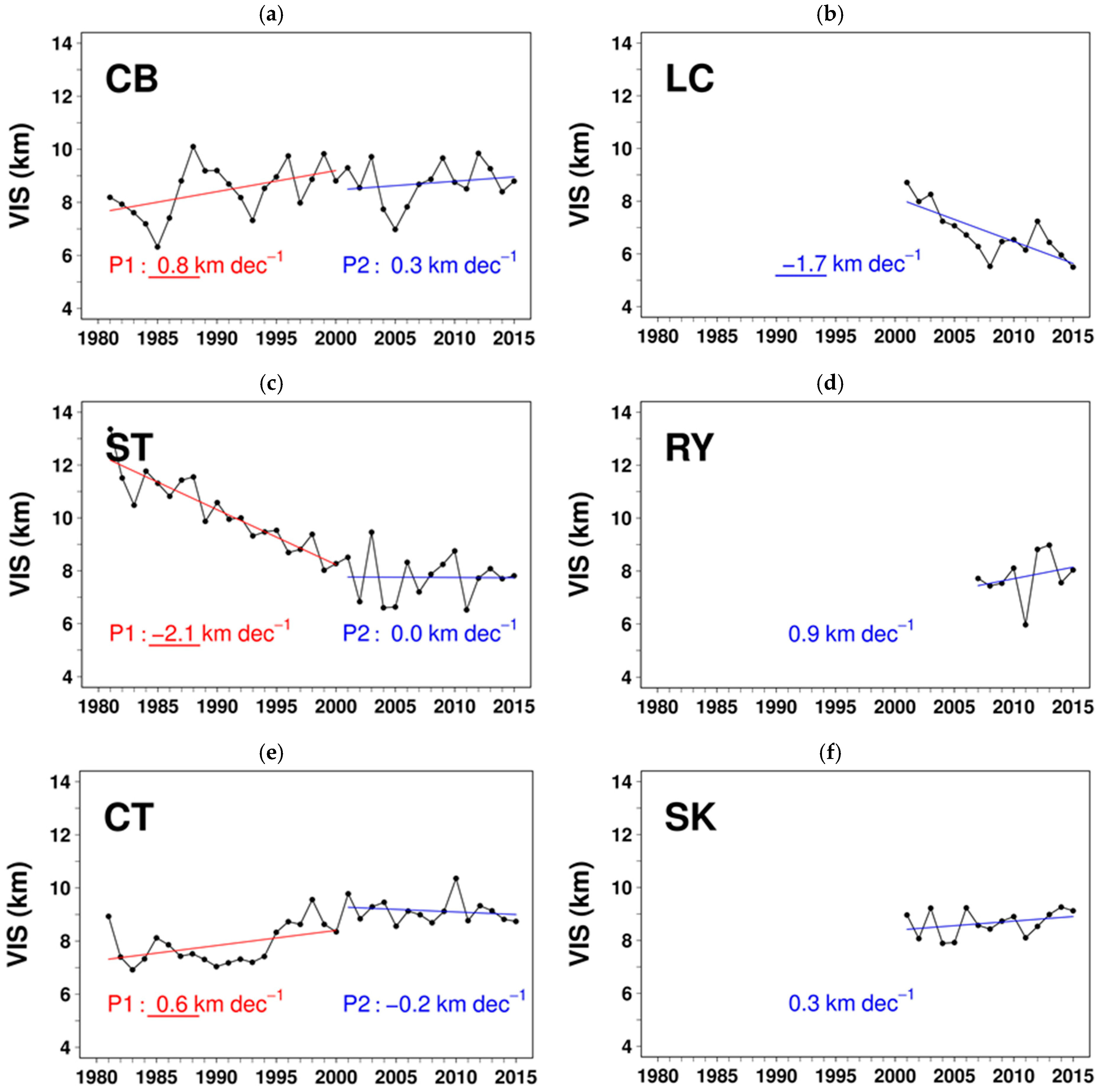
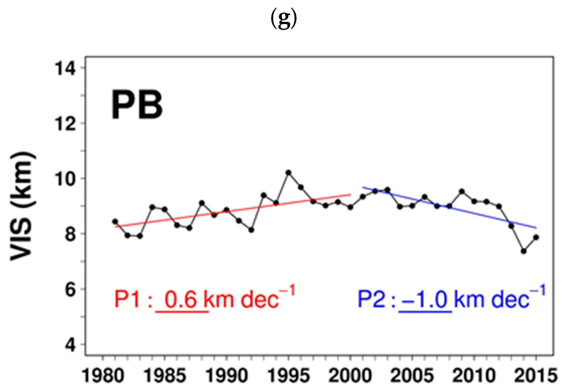
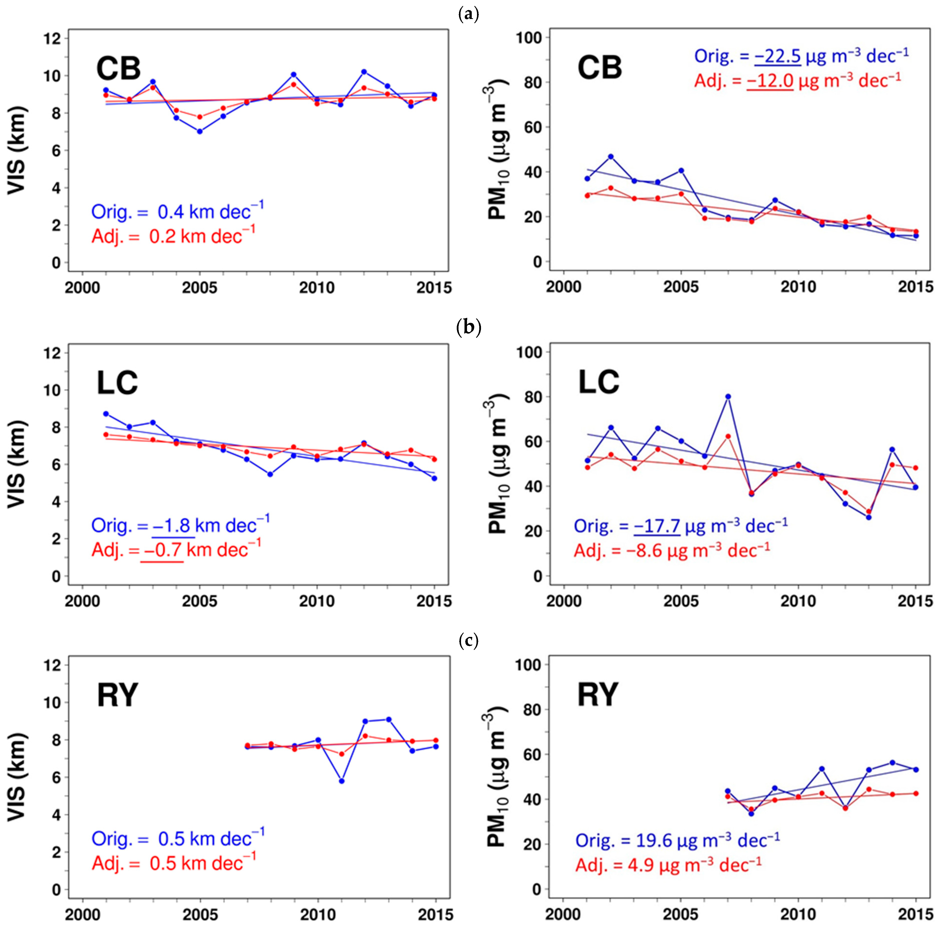
3.6. Trends and Meteorological Adjustment for Visibility and PM₁₀

Station CB has a significant positive (increasing) trend in visibility in the P1 period (0.8 km dec⁻¹, where “dec” denotes decade); however, its magnitude becomes smaller and also insignificant in the P2 period (0.3 km dec⁻¹). Visibility at LC declines significantly in the P2 period (−1.7 km dec⁻¹) while the trends at ST significantly decline in the P1 period (−2.1 km dec⁻¹); however, it becomes persistently low in the P2 period. Although the trends at RY and SK are positive, they are not significant. At both CT and PB, the trends are once significantly positive (0.6 km dec⁻¹); however, they become negative over recent years (significantly in the case of PB, −1.0 km dec⁻¹) (Figure 9). All of the four stations with the long-term visibility data display either a negative shift of trend (from the P1 to P2 periods) or persistent low visibility due to their proximity to urban and/or industrial areas. Station LC has the fastest decline of visibility over the recent period. The insignificant trend in visibility over SK could be due to a rural background and not much change in anthropogenic activities. Since the time span for trend calculation is limited (nine years) at RY, not much can be established from it.

The results of trend and meteorological adjustment for CB, LC, and RY are shown in Figure 10. The final fitted GLM explained 41.2%, 59.7% and 51.9% of total variance in visibility for CB, LC and RY, respectively. For PM₁₀, the final GLM fit explained 62.7%, 53.9% and 49.7% of total variance. All the fitted models were found to be acceptable in terms of residual diagnostics. Notice that the adjusted trends tend to fluctuate less year-to-year than the original trends, which is due to the fact that substantial inter-annual variability resulting from meteorology was already removed. Here, our discussion focuses specifically on the adjusted trends (as better reflecting the anthropogenic signature or influence than the original ones, and more policy-relevant). At CB, PM₁₀ level decreases significantly at the rate of −12 μg m⁻³ dec⁻¹, suggestive of local primary emissions being reduced over time. However, the visibility trend is insignificant (0.2 km dec⁻¹). At LC, adjusted visibility and PM₁₀ level show contrasting trends. Visibility has decreased sharply at −0.7 km dec⁻¹, while PM₁₀ shows an insignificant decreasing trend (−8.6 μg m⁻³ dec⁻¹). The potential cause and linkage that may help explain such contrast, at least in part, is the formation of secondary aerosols. In the previous section (Section 3.5), we found secondary aerosols to be associated with visibility. Such secondary aerosols are in fact fine particles to which visibility or optical extinction is sensitive, and they are not readily represented by PM₁₀. Contrasting trends in visibility and PM₁₀ have also been reported in some other studies [10,15]. At RY, the time coverage is relatively short (nine years, generally not very adequate for trend estimation). We found that both visibility and PM₁₀ level do not have any significant trends. Based on the adjusted trend results discussed, none of the visibility trends are significantly positive, while some are in contrast with those of PM₁₀. These results indicate that meteorology affects trends in both visibility and PM₁₀. The results also suggest that the trend in fine particulate matter (PM_2.5) could correlate better with the trend in visibility.

4. Conclusions

Observed long-term visibility in the eastern region of Thailand was studied, with the focus on its urbanized/highly industrialized coastal areas, using weather data from seven stations with a temporal coverage of 35 years (1981–2015) for four stations, 15 years (2001–2015) for two stations, and nine years (2007–2015) for one station. The relationship between visibility and air pollutants was also investigated using air quality data from five stations (15 years for three stations and seven years for two stations). Visibility shows strong seasonality and its degradation intensifies in the dry season due to increased air pollution as well as due to certain favorable meteorological conditions such as low wet scavenging, reduced mixing height, and increased recirculation factor. Visibility showed negative correlation with PM₁₀ which is evident with correlation analysis, class-wise comparison and weekday-weekend differences. Visibility showed negative correlation coefficient of −0.29 (−0.22), −0.32 (−0.23) and −0.51 (−0.64) with PM₁₀ on daily (monthly scale) for CB, LC and RY, respectively. Mean level of PM₁₀ under poor visibility condition (Class III) was around 1.6–1.7 times higher than in good visibility condition (Class I). Average visibility was 9.1 km, 7.1 km and 8.2 km during the weekend and 8.6 km, 6.8 km and 7.6 km during the weekdays for CB, LC and RY due to a higher mean level of PM₁₀ during the weekdays. The results from the equal step-size method showed a negative relation between visibility and RH with the effect of hygroscopic growth of aerosol being a more dominating process as compared to a change in size distribution of dry particles. The strong dependency of visibility on wind direction with relatively lower visibility with wind prevailing from sources of local pollution is indicative of the influence of local pollution sources. The back-trajectory results showed relatively lower visibility with the northeasterly clusters, which represent continental air masses and brings polluted air from inland areas. The effect of air pollution and humidity is not readily discerned for undefined clusters. These evidently suggest the important influences of the long-range transport of pollutants and humidity on visibility. The precursor ratio method showed an increase in the formation of sulfate, nitrate and secondary organic aerosol under low visibility conditions, suggesting their potential role in visibility degradation. Among these precursors, the formation of sulfate from SO₂ seems to play the most important role in visibility degradation. This highlights the importance of controlling the gaseous precursors of secondary aerosols for visibility improvement in the region. Trend analysis of average visibility shows a negative shift in trend, decreasing trend, or persistence of relatively low visibility over most of the stations, raising an environmental concern and suggesting a need for more attention from policymakers and air quality workers. The contrasting trends in visibility and PM₁₀ level after the GLM-based meteorological adjustment are partly attributed to the role of fine particles, to which visibility is more sensitive. This study provides empirical evidence that visibility is impacted by secondary aerosols, which would be warranted concretely by taking into account fine particulate matter (e.g., PM_2.5) data and their chemical components, which were not available in this study. Continued investigation on visibility in the eastern region of Thailand or extension to other areas can broaden the understanding of visibility quality at a regional scale. Linking visibility to synoptic circulation patterns can enhance the current observational analysis framework. Advanced air quality modeling and source apportionment for visibility can be utilized to specifically determine emission sources contributing to visibility degradation. Given that human-based visibility observation has its own limitation in terms of uncertainty and reliability, automated visibility measurement may offer an alternative source of data for future comparison and application, as the TMD has recently installed automated visibility sensors at its standard weather stations although only at a small number of stations. Based on the results in this study, we recommend: (a) Apart from particulate pollution, emissions of precursor gases for secondary aerosols should also be paid attention to improve visibility. (b) Regional transport of air pollutants also play important role in visibility degradation posing a challenge to its improvement with the measures of reducing local emission. (c) The negative trends and persistently low tendency in visibility over the past years provide a clear evidence to policy makers regarding the impact of industrialization and urbanization. Given that there is a larger-scale regional developers (i.e., Eastern Economic Corridor), the awareness of visibility degradation should be integrated into policy making. (d) Policy makers should also think about amenity effects of higher air pollution apart from the health effects while deciding the framework for managing air quality.

References

1. Seinfeld, J.H.; Pandis, S.N. Atmospheric Chemistry and Physics from Air Pollution to Climate Change, 2nd ed.; John Wiley & Sons, Inc.: New York, NY, USA, 2006; ISBN 9780471720171. [Google Scholar]
2. Watson, J.G. Visibility: Science and regulation. J. Air Waste Manag. Assoc. 2002, 52, 628–713. [Google Scholar] [CrossRef] [PubMed]
3. Boylan, J.W.; Odman, M.T.; Wilkinson, J.G.; Russell, A.G. Integrated Assessment Modeling of Atmospheric Pollutants in the Southern Appalachian Mountains: Part II. Fine Particulate Matter and Visibility. J. Air Waste Manag. Assoc. 2006, 56, 12–22. [Google Scholar] [CrossRef] [PubMed] [Green Version]
4. Zhang, Q.H.; Zhang, J.P.; Xue, H.W. The challenge of improving visibility in Beijing. Atmos. Chem. Phys. 2010, 10, 7821–7827. [Google Scholar] [CrossRef] [Green Version]
5. Sloane, C.S. Visibility trends-I. Methods of analysis. Atmos. Environ. 1982, 16, 41–51. [Google Scholar] [CrossRef]
6. Singh, A.; Bloss, W.J.; Pope, F.D. 60 years of UK visibility measurements: Impact of meteorology and atmospheric pollutants on visibility. Atmos. Chem. Phys. 2017, 17, 2085–2101. [Google Scholar] [CrossRef]
7. Tsai, Y.I. Atmospheric visibility trends in an urban area in Taiwan 1961–2003. Atmos. Environ. 2005, 39, 5555–5567. [Google Scholar] [CrossRef]
8. Fu, W.; Chen, Z.; Zhu, Z.; Liu, Q.; Qi, J.; Dang, E.; Wang, M.; Dong, J. Long-term atmospheric visibility trends and characteristics of 31 provincial capital cities in China during 1957–2016. Atmosphere 2018, 9, 318. [Google Scholar] [CrossRef]
9. Majewski, G.; Rogula-Kozlowska, W.; Czechowski, P.O.; Badyda, A.; Brandyk, A. The impact of selected parameters on visibility: First results from a long-term campaign in Warsaw, Poland. Atmosphere 2015, 6, 1154–1174. [Google Scholar] [CrossRef]
10. Chen, Y.; Xie, S. Long-term trends and characteristics of visibility in two megacities in southwest China: Chengdu and Chongqing. J. Air Waste Manag. Assoc. 2013, 63, 1058–1069. [Google Scholar] [CrossRef] [PubMed] [Green Version]
11. Pengchai, P.; Chantara, S.; Sopajaree, K.; Wangkarn, S.; Tengcharoenkul, U.; Rayanakorn, M. Seasonal variation, risk assessment and source estimation of PM10 and PM10-bound PAHs in the ambient air of Chiang Mai and Lamphun, Thailand. Environ. Monit. Assess. 2009, 154, 197–218. [Google Scholar] [CrossRef] [PubMed]
12. Wen, C.C.; Yeh, H.H. Comparative influences of airborne pollutants and meteorological parameters on atmospheric visibility and turbidity. Atmos. Res. 2010, 96, 496–509. [Google Scholar] [CrossRef]
13. Quan, J.; Tie, X.; Zhang, Q.; Liu, Q.; Li, X.; Gao, Y.; Zhao, D. Characteristics of heavy aerosol pollution during the 2012–2013 winter in Beijing, China. Atmos. Environ. 2014, 88, 83–89. [Google Scholar] [CrossRef]
14. Wang, K.; Dickinson, R.E.; Liang, S. Clear sky visibility has decreased over land globally from 1973 to 2007. Science 2009, 323, 1468–1470. [Google Scholar] [CrossRef] [PubMed]
15. Wang, K.C.; Dickinson, R.E.; Su, L.; Trenberth, K.E. Contrasting trends of mass and optical properties of aerosols over the Northern Hemisphere from 1992 to 2011. Atmos. Chem. Phys. 2012, 12, 9387–9398. [Google Scholar] [CrossRef] [Green Version]
16. Hu, Y.; Yao, L.; Cheng, Z.; Wang, Y. Long-term atmospheric visibility trends in megacities of China, India and the United States. Environ. Res. 2017, 159, 466–473. [Google Scholar] [CrossRef] [PubMed]
17. Sabetghadam, S.; Ahmadi-Givi, F.; Golestani, Y. Visibility trends in Tehran during 1958–2008. Atmos. Environ. 2012, 62, 512–520. [Google Scholar] [CrossRef]
18. Assareh, N.; Prabamroong, T.; Manomaiphiboon, K.; Theramongkol, P.; Leungsakul, S.; Mitrjit, N.; Rachiwong, J. Analysis of observed surface ozone in the dry season over Eastern Thailand during 1997–2012. Atmos. Res. 2016, 178–179, 17–30. [Google Scholar] [CrossRef]
19. Chusai, C.; Manomaiphiboon, K.; Saiyasitpanich, P.; Thepanondh, S. NO2 and SO2 dispersion modeling and relative roles of emission sources over Map Ta Phut industrial area, Thailand. J. Air Waste Manag. Assoc. 2012, 62, 932–945. [Google Scholar] [CrossRef] [PubMed]
20. Pollution Control Department (PCD). Thailand State of Pollution 2015; Pollution Control Department: Bangkok, Thailand, 2016. Available online: http://infofile.pcd.go.th/mgt/PollutionReport2015_en.pdf (accessed on 19 September 2017).
21. Pimpisut, D.; Jinsart, W.; Hooper, M.A. Modeling of the BTX species based on an emission inventory of sources at the Map Ta Phut industrial estate in Thailand. Sci. Asia 2005, 31, 103–112. [Google Scholar] [CrossRef]
22. Prabamroong, T.; Manomaiphiboon, K.; Limpaseni, W.; Sukhapan, J.; Bonnet, S. Ozone and its potential control strategy for Chon Buri city, Thailand. J. Air Waste Manag. Assoc. 2012, 62, 1411–1422. [Google Scholar] [CrossRef] [PubMed] [Green Version]
23. Singkaew, P.; Kongtip, P.; Yoosook, W.; Chantanakul, S. Health risk assessment of volatile organic compounds in a high risk group surrounding Map Ta Phut industrial estate, Rayong Province. J. Med. Assoc. Thail. 2013, 96 (Suppl. 5), S73–S81. [Google Scholar]
24. National Economic and Social Development Board (NESDB). Gross Regional and Provincial Product, Chain Volume Measures 2015 Edition; Office of the National Economic and Social Development Board: Bangkok, Thailand, 2017. Available online: http://www.nesdb.go.th/nesdb_en/ewt_dl_link.php?nid=4317 (accessed on 15 May 2018).
25. National Economic and Social Development Board (NESDB). Gross Regional and Provincial Products (1981–1995 and 1995–2011); Office of the National Economic and Social Development Board: Bangkok, Thailand, 2016. Available online: http://www.nesdb.go.th/nesdb_en/ewt_news.php?nid=4315&filename=national_account (accessed on 1 December 2016).
26. National Statistical Office (NSO). Gross Regional and Provincial Products (2005–2015); National Statistical Office: Bangkok, Thailand, 2016. Available online: http://service.nso.go.th/nso/web/statseries/statseries15.html (accessed on 1 December 2016).
27. Khantaraphan, U. Smoggy Day in Pattaya. Pattaya Mail (30 September 2015). 2015. Available online: http://www.pattayamail.com/news/smoggy-day-in-pattaya-51691 (accessed on 15 May 2018).
28. Industrial Estate Authority of Thailand (IEAT). Annual Report 2016. Industrial Estate Authority of Thailand; 2017. Available online: http://www.ieat.go.th/assets/uploads/cms/file/201709081923251820708181.pdf (accessed on 15 May 2018).
29. Khuntong, S.; Wongsorntam, K.; Thepanondh, S.; Khaenamkaew, P. Effect of particulate matters from shipping activities around Si Racha Bay Si Chang Island. Environ. Asia 2010, 3, 59–68. [Google Scholar]
30. Pham, T.B.T.; Manomaiphiboon, K.; Vongmahadlek, C. Development of an inventory and temporal allocation profiles of emissions from power plants and industrial facilities in Thailand. Sci. Total Environ. 2008, 397, 103–118. [Google Scholar] [CrossRef] [PubMed]
31. Ruangjun, S.; Exell, R.H.B. Regression models for forecasting fog and poor visibility at Don muang airport in winter. Asian J. Energy Environ. 2008, 9, 215–230. [Google Scholar]
32. Vajanapoom, N.; Shy, C.M.; Neas, L.M.; Loomis, D. Estimation of particulate matter from visibility in Bangkok, Thailand. J. Expo. Anal. Environ. Epidemiol. 2001, 11, 97–102. [Google Scholar] [CrossRef] [PubMed] [Green Version]
33. Janjai, S.; Kumharn, W.; Laksanaboonsong, J. Determination of Angstrom’s turbidity coefficient over Thailand. Renew. Energy 2003, 28, 1685–1700. [Google Scholar] [CrossRef]
34. Land Development Department (LDD). Land Use and Land Cover Data for Thailand for the Years 2006–2007; CD-ROM Product; Land Development Department: Bangkok, Thailand, 2007.
35. Thai Meteorological Department (TMD). The Climate of Thailand; Thai Meteorological Department: Bangkok, Thailand, 2016. Available online: https://www.tmd.go.th/en/archive/thailand_climate.pdf (accessed on 1 December 2016).
36. Phan, T.T.; Manomaiphiboon, K. Observed and simulated sea breeze characteristics over Rayong coastal area, Thailand. Meteorol. Atmos. Phys. 2012, 116, 95–111. [Google Scholar] [CrossRef]
37. Reeves, J.; Chen, J.; Wang, X.L.; Lund, R.; Lu, Q.Q. A review and comparison of changepoint detection techniques for climate data. J. Appl. Meteorol. Climatol. 2007, 46, 900–915. [Google Scholar] [CrossRef]
38. Ross, G. Parametric and nonparametric sequential change detection in R: The CPM package. J. Stat. Softw. 2015, 66, 3. [Google Scholar]
39. Zahumenský, I. Guidelines on Quality Control Procedures for Data from Automatic Weather Stations. World Meteorol. Organ. 2004. Available online: https://www.wmo.int/pages/prog/www/IMOP/meetings/Surface/ET-STMT1_Geneva2004/Doc6.1(2).pdf (accessed on 19 September 2017).
40. Allwine, K.J.; Whiteman, C.D. Single-station integral measures of atmospheric stagnation, recirculation and ventilation. Atmos. Environ. 1994, 28, 713–721. [Google Scholar] [CrossRef]
41. US Environmental Protection Agency (US EPA). User’s Guide for the AERMOD Meteorological Preprocessor (AERMET). Res. Triangle Park. NC, Off. Air Qual. 2004. Report No. EPA-454/B-03-002. Available online: https://www3.epa.gov/scram001/7thconf/aermod/aermetugb.pdf (accessed on 19 September 2018).
42. Sloane, C.S. Visibility trends-II. Mideastern United States 1948–1978. Atmos. Environ. 1982, 16, 2309–2321. [Google Scholar] [CrossRef]
43. US Environmental Protection Agency (US EPA). Characterizing Visibility Trends: A Review of Historical Approaches and Recommendation for Future Analyses; US EPA: Washington, DC, USA, 1987.
44. Rosenfeld, D.; Dai, J.; Yu, X.; Yao, Z.; Xu, X.; Yang, X.; Du, C. Inverse relations between amounts of air pollution and orographic precipitation. Science 2007, 315, 1396–1398. [Google Scholar] [CrossRef] [PubMed]
45. Founda, D.; Kazadzis, S.; Mihalopoulos, N.; Gerasopoulos, E.; Lianou, M.; Raptis, P.I. Long-term visibility variation in Athens (1931–2013): A proxy for local and regional atmospheric aerosol loads. Atmos. Chem. Phys. 2016, 16, 11219–11236. [Google Scholar] [CrossRef]
46. Kasten, F. Visibility forecast in the phase of pre-condensation. Tellus 1969, 1969. 5, 631–635. [Google Scholar]
47. Meszaros, A. An attempt to explain the relation between visual range and relative humidity on the basis of aerosol measurements. J. Aerosol Sci. 1977, 8, 31–38. [Google Scholar] [CrossRef]
48. Fitzgerald, J.; Hoppel, A.; Vietti, M.A. The size and scattering coefficient of urban aerosol particles at Washington, DC as a function of relative humidity. J. Atmos. Sci. 1982, 39, 1838–1852. [Google Scholar] [CrossRef]
49. Davies, C.N. Visual Range and size of atmospheric particles. J. Aerosol Sci. 1975, 6, 335–347. [Google Scholar] [CrossRef]
50. Carslaw, D.C.; Ropkins, K. Openair—An R package for air quality data analysis. Environ. Model. Softw. 2012, 27–28, 52–61. [Google Scholar] [CrossRef]
51. Aneja, V.P.; Brittig, J.S.; Kim, D.; Carolina, N. Ozone and other air quality-related variables affecting visibility in the Southeast United States. J. Air Waste Manag. Assoc. 2004, 54, 681–688. [Google Scholar] [CrossRef] [PubMed]
52. Pitchford, M.; Pitchford, A. Analysis of regional visibility in the southwest using principal component and back trajectory techniques. Atmos. Environ. 1985, 19, 1301–1316. [Google Scholar] [CrossRef]
53. Stohl, A.; Wotawa, G.; Seibert, P.; Kromp-Kolb, H. Interpolation Errors in Wind Fields as a Function of Spatial and Temporal Resolution and Their Impact on Different Types of Kinematic Trajectories. J. Appl. Meteorol. 1995, 34, 2149–2165. [Google Scholar] [CrossRef] [Green Version]
54. Saha, S.; Moorthi, S.; Pan, H.L.; Wu, X.; Wang, J.; Nadiga, S.; Tripp, P.; Kistler, R.; Woollen, J.; Behringer, D.; et al. The NCEP climate forecast system reanalysis. Bull. Am. Meteorol. Soc. 2010, 91, 1015–1057. [Google Scholar] [CrossRef]
55. Wilks, D.S. Statistical Methods in the Atmospheric Sciences, 2nd ed.; International Geophysics Series; Elsevier: London, UK, 2006. [Google Scholar]
56. R Development Core Team. R: A Language and Environment for Statistical Computing (Version 3.1.0); R Foundation for Statistical Computing: Vienna, Austria, 2014. [Google Scholar]
57. Zhang, Y.L.; Cao, F. Fine particulate matter (PM2.5) in China at a city level. Sci. Rep. 2015, 5, 14884. [Google Scholar] [CrossRef] [PubMed]
58. Yue, S.; Pilon, P. A comparison of the power of the t test, Mann-Kendall and bootstrap tests for trend detection. Hydrol. Sci. J. 2004, 49, 21–37. [Google Scholar] [CrossRef]
59. Camalier, L.; Cox, W.; Dolwick, P. The effects of meteorology on ozone in urban areas and their use in assessing ozone trends. Atmos. Environ. 2007, 41, 7127–7137. [Google Scholar] [CrossRef]
60. Barmpadimos, I.; Hueglin, C.; Keller, J.; Henne, S.; Prévôt, A.S.H. Influence of meteorology on PM10 trends and variability in Switzerland from 1991 to 2008. Atmos. Chem. Phys. 2011, 11, 1813–1835. [Google Scholar] [CrossRef]
61. Wise, E.K.; Comrie, A.C. Meteorologically adjusted urban air quality trends in the Southwestern United States. Atmos. Environ. 2005, 39, 2969–2980. [Google Scholar] [CrossRef]
62. Giglio, L.; Csiszar, I.; Justice, C.O. Global distribution and seasonality of active fires as observed with the Terra and Aqua Moderate Resolution Imaging Spectroradiometer (MODIS) sensors. J. Geophys. Res. Biogeosci. 2006, 111, G02016. [Google Scholar] [CrossRef]
63. Xu, W.Y.; Zhao, C.S.; Ran, L.; Lin, W.L.; Yan, P.; Xu, X.B. SO2 noontime-peak phenomenon in the North China Plain. Atmos. Chem. Phys. 2014, 14, 7757–7768. [Google Scholar] [CrossRef]
64. Li, M.; Zhang, Q.; Kurokawa, J.I.; Woo, J.H.; He, K.; Lu, Z.; Ohara, T.; Song, Y.; Streets, D.G.; Carmichael, G.R.; et al. MIX: A mosaic Asian anthropogenic emission inventory under the international collaboration framework of the MICS-Asia and HTAP. Atmos. Chem. Phys. 2017, 17, 935–963. [Google Scholar] [CrossRef]
Figure 1. (a) Thailand; (b) eastern region and its provinces, and (c) monitoring stations. In (b), built-up areas are shaded grey, representing urban, residential, industrial, and commercial areas combined based on Land Development Department (LDD) (2007) [34]. In (c), for some Thai Meteorological Department (TMD) and Pollution Control Department (PCD) stations being very close to each other, only one filled circle is given. CB (Chon Buri), LC (Laem Chabang), and RY (Rayong) (in boxes) denote the most important TMD stations in the analysis, which are paired with nearby PCD stations for air quality data (here, P1 (General Education Office), P2 and P3 (Sri Racha Juvenile Center and Kasetsart University Sri Racha), and P4 and P5 (Rayong Field Crops Research Center and Map Ta Phut Health Center), respectively).
Atmosphere 10 00122 g001
Figure 2. (a) gross provincial product (GPP) (at current market price); (b) fuel consumption (ktoe, 1 ktoe = 41,868 × 109 J); and (c) registered population for Chon Buri and Rayong provinces, Thailand.
Atmosphere 10 00122 g002
Figure 3. Monthly variation of (a) visibility (before met-screening); (b) visibility; (c) PM10; (d) rain; (e) relative humidity; (f) temperature; (g) wind speed; (h) mixing height; (i) global radiation; and (j) recirculation factor.
Atmosphere 10 00122 g003aAtmosphere 10 00122 g003b
Figure 4. (a) average PM10 by visibility class and by station, and (bd) average visibility, relative humidity (RH)-corrected visibility, and PM10, respectively, at stations CB, LC, and RY during the weekdays (Monday–Saturday) and the weekend (Sunday plus holidays). The difference in any pair of mean values in the above results is statistically significant at the 0.05 level.
Atmosphere 10 00122 g004
Figure 5. Average visibility, RH-corrected visibility and PM10 under different RH intervals at (a) Chon Buri (CB); (b) Laem Chabang (LC); and (c) Rayong (RY).
Atmosphere 10 00122 g005
Figure 6. Polar plots of visibility (VIS), visibility/RH-corrected visibility (VIS/VISd), and PM10 at (a) Chon Buri (CB); (b) Laem Chabang (LC); and (c) Rayong (RY).
Atmosphere 10 00122 g006
Figure 7. Average back-trajectory path and its average height by cluster at stations (a) CB and LC; and (b) RY.
Atmosphere 10 00122 g007
Figure 8. (a) PM10/CO (µg m−3 ppm−1); (b) SO2/CO (ppb ppm−1); (c) NOx/CO (ppb ppm−1); and (d) NMHC/CO (ppbc ppm−1) by visibility class at stations CB, LC, and RY.
Atmosphere 10 00122 g008
Figure 9. Trends in visibility at (a) Chon Buri (CB); (b) Laem Chabang (LC); (c) Sattahip (ST); (d) Rayong (RY); (e) Chanthaburi (CT); (f) Sa Kaeo (SK); (g) Prachin Buri (PB). For CB, ST, CT, and PB, the red and blue lines are the linear fits over the periods of 1981–2000 and 2001–2015, respectively. For the other stations, the linear fits are limited to recent years (here, 2001 or after). The underlined values are of statistical significance at a 0.05 level against the null hypothesis of no trend.
Atmosphere 10 00122 g009aAtmosphere 10 00122 g009b
Figure 10. Meteorologically adjusted (red) and original or non-adjusted (blue) trends in visibility and PM10 at (a) Chon Buri (CB); (b) Laem Chabang (LC); (c) Rayong (RY). The underlined values are of statistical significance at a 0.05 level against the null hypothesis of no trend. At each station, the trend period was determined by the time coverage of the visibility and air quality data available and considered.
Atmosphere 10 00122 g010