Numerical Investigations of Atmospheric Rivers and the Rain Shadow over the Santa Clara Valley


Abstract
1. Introduction
2. Data and Methods
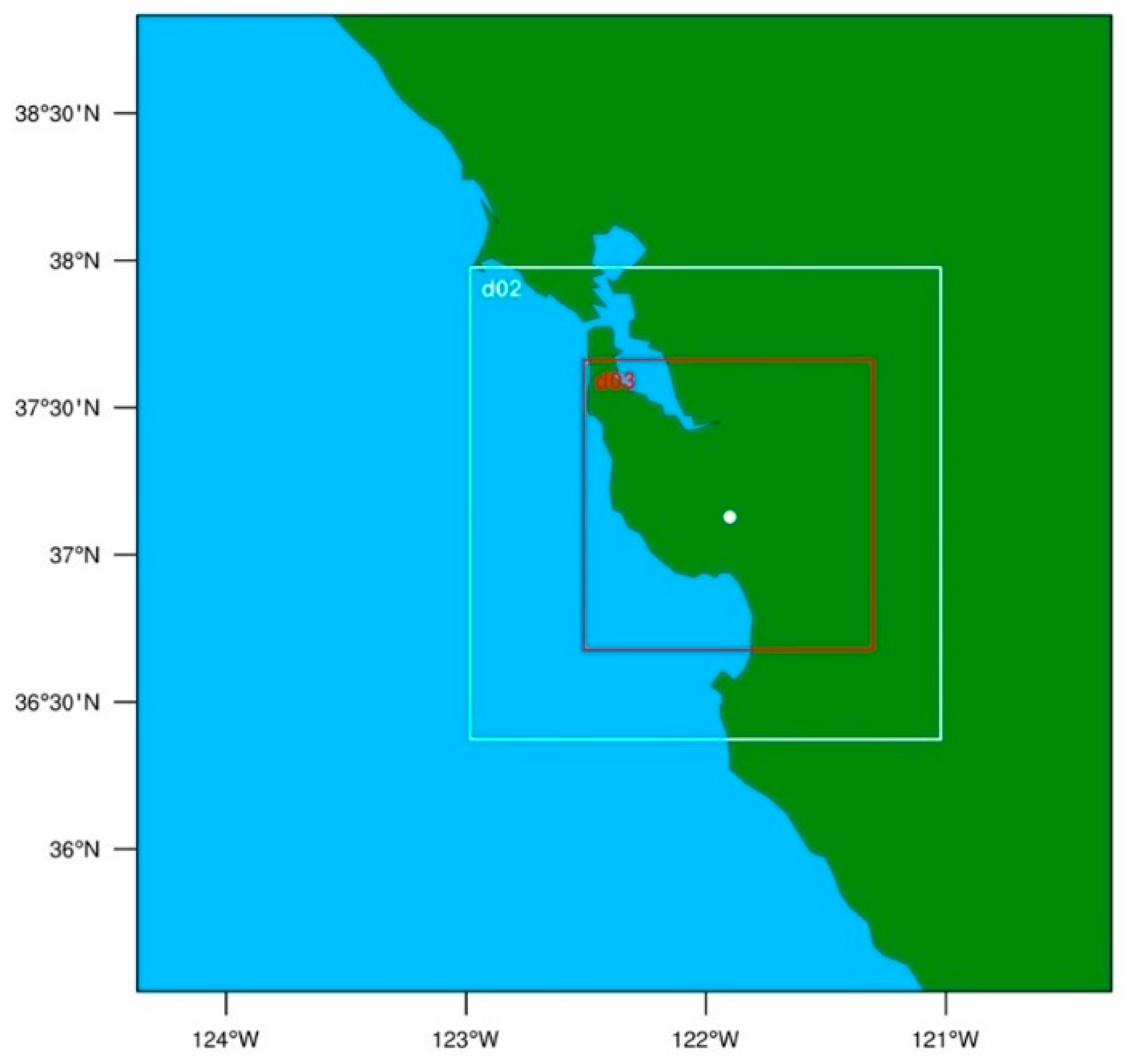
2.1. Model Setup
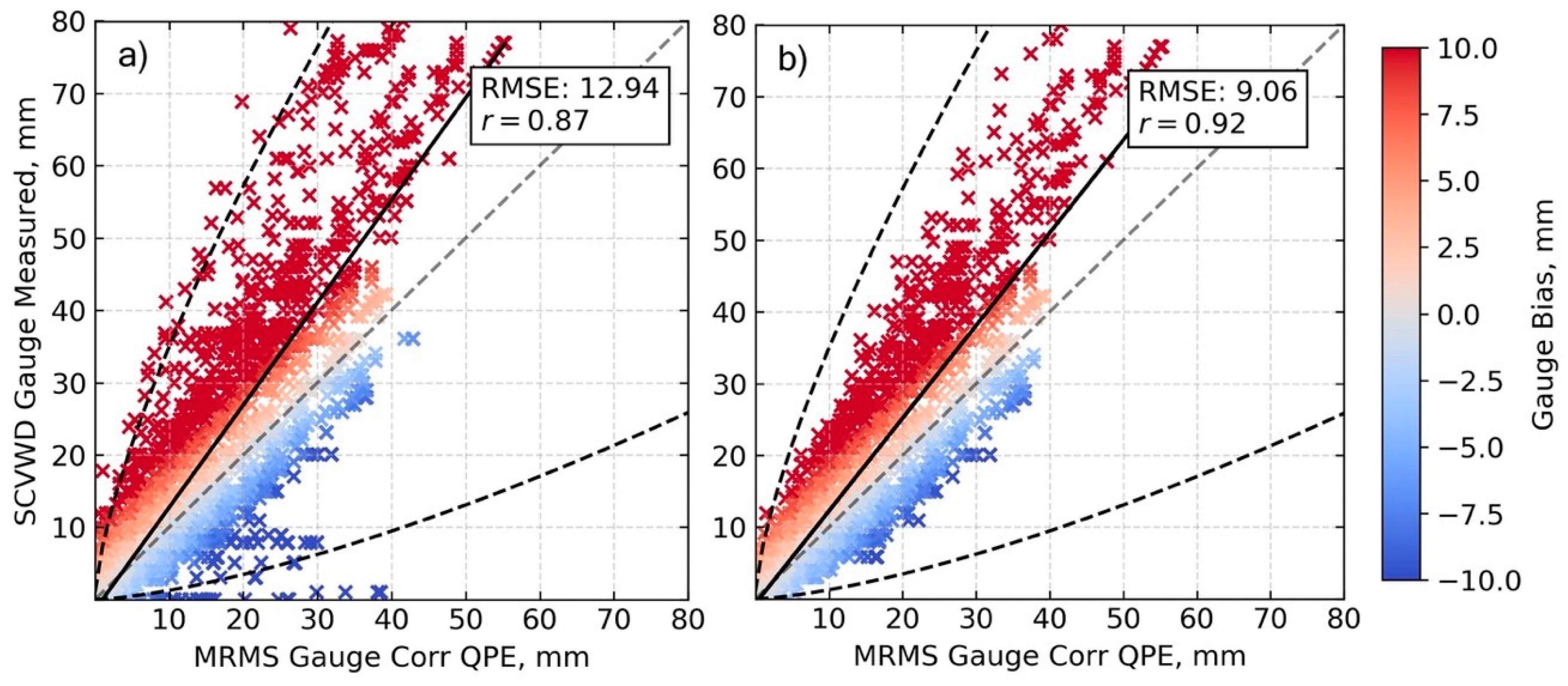
2.2. Radar Observations
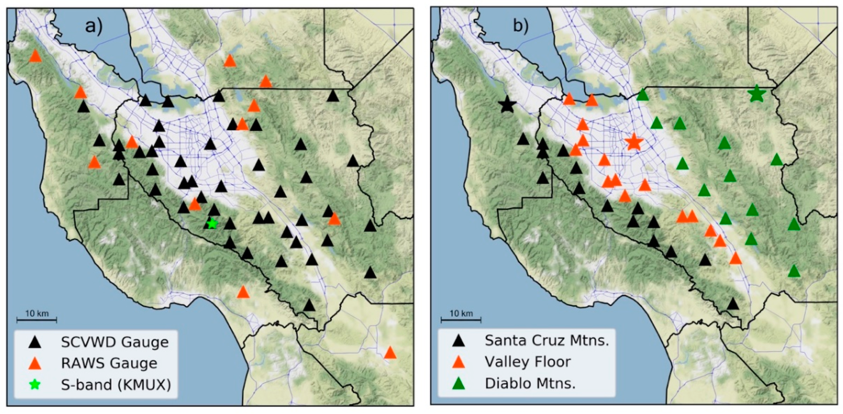
2.3. Surface Observations
2.4. Description of Events
3. Results
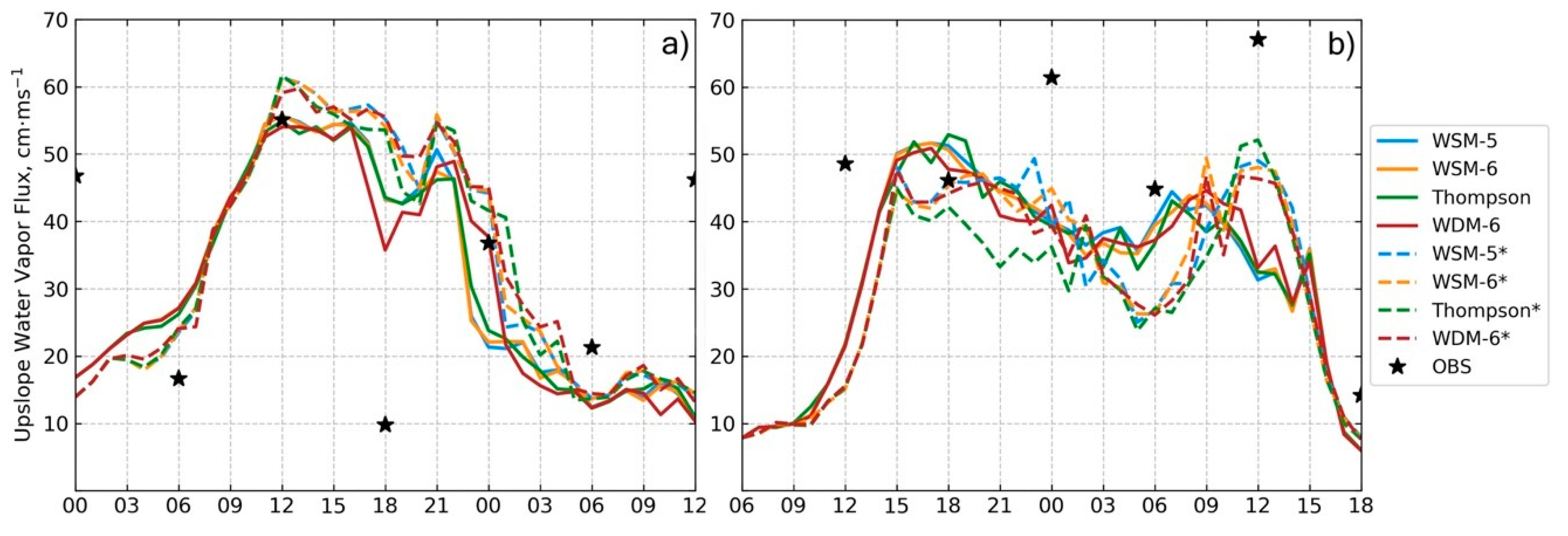
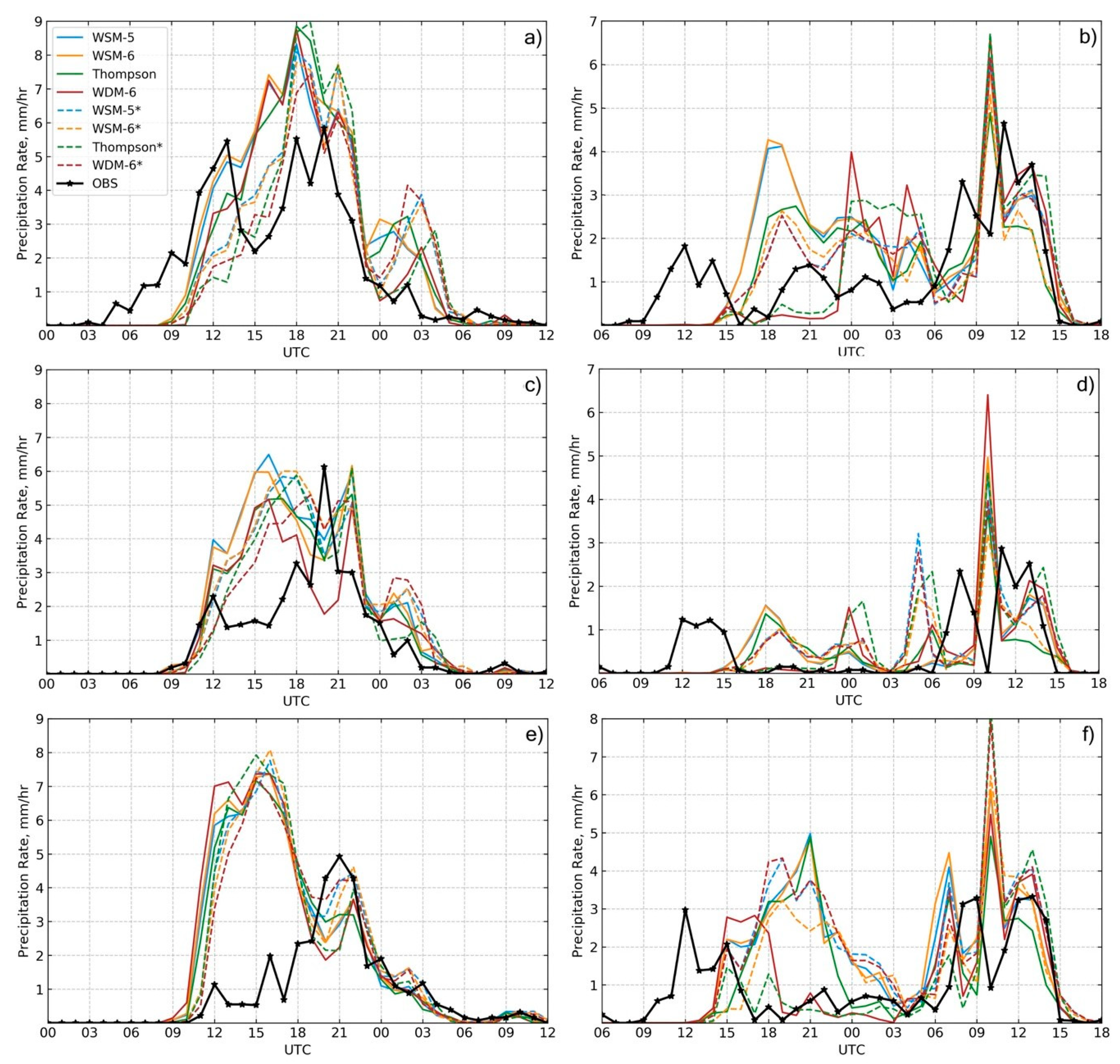
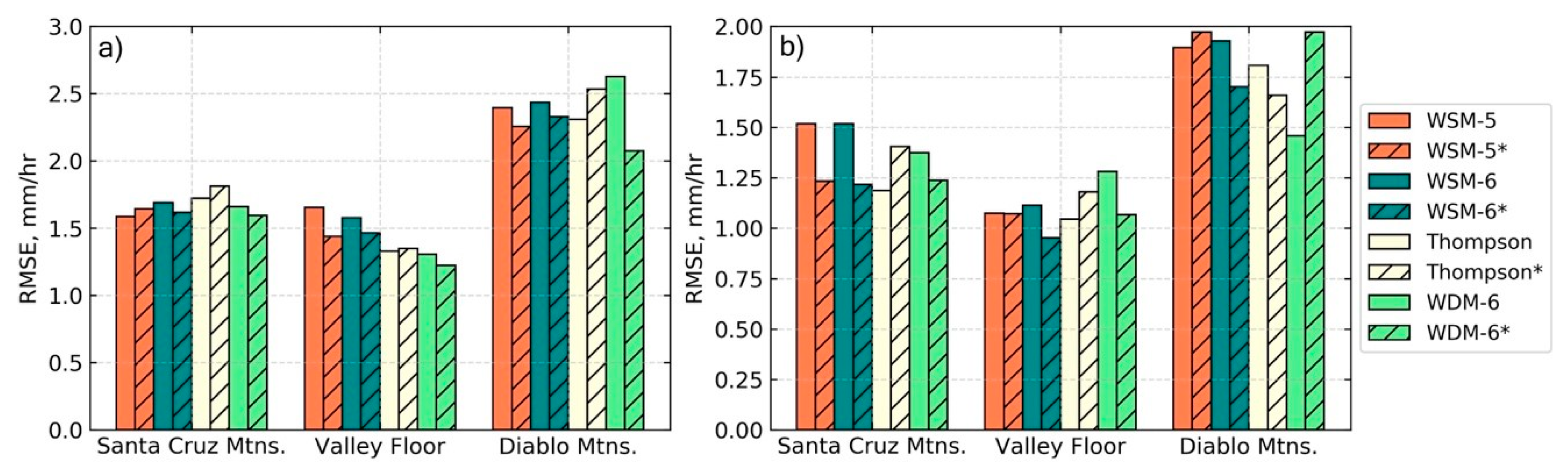
3.1. Simulated Precipitation
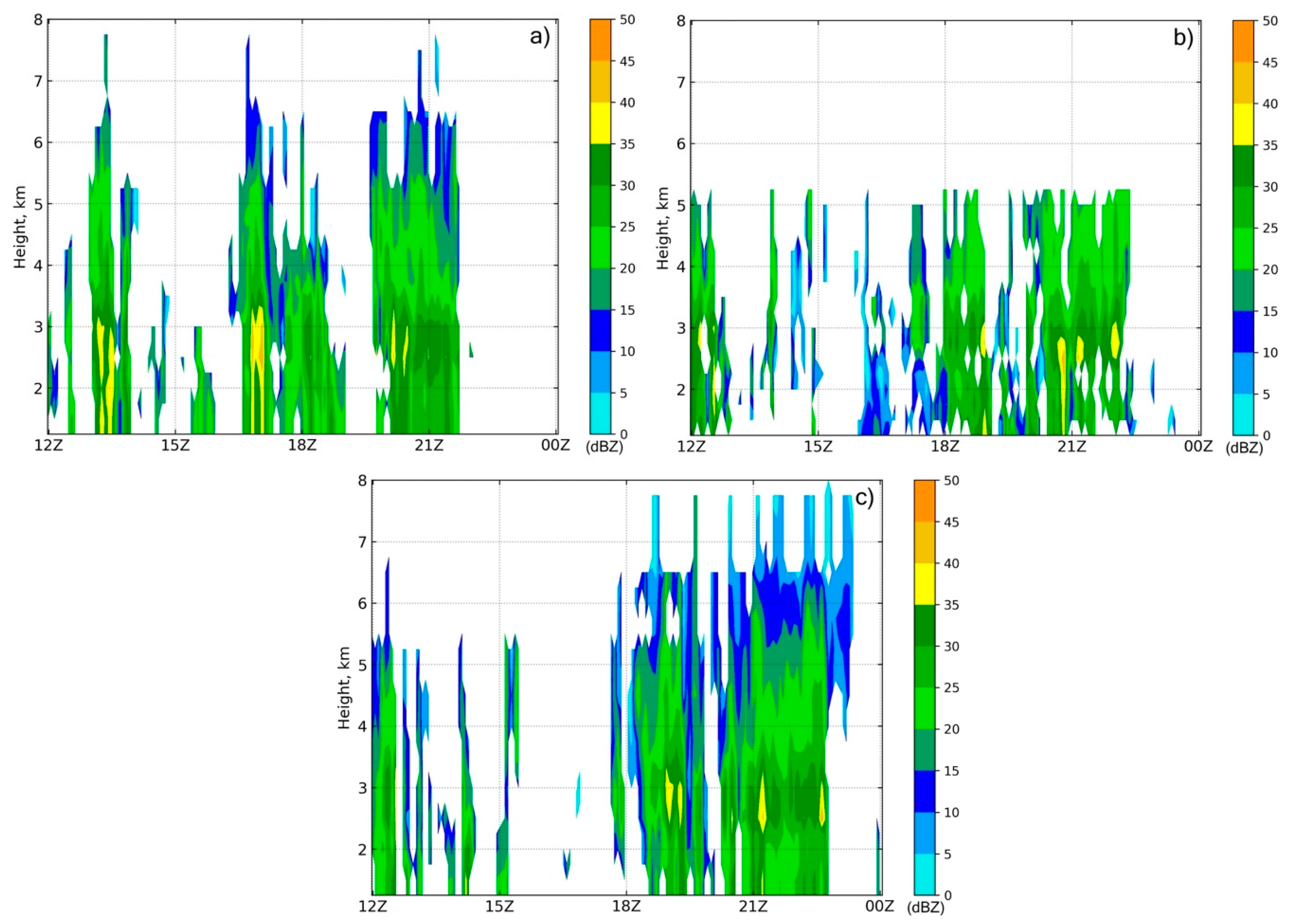
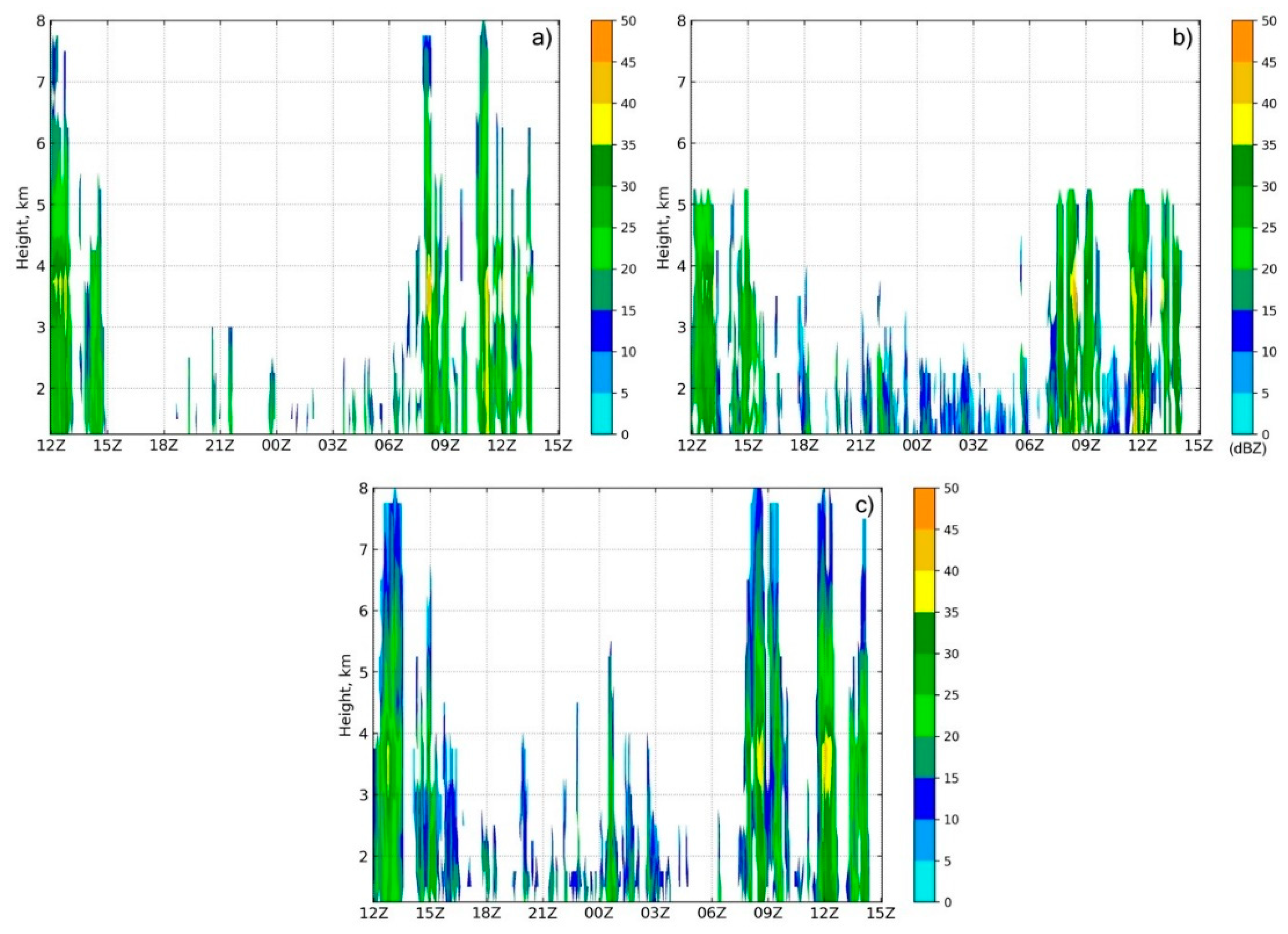
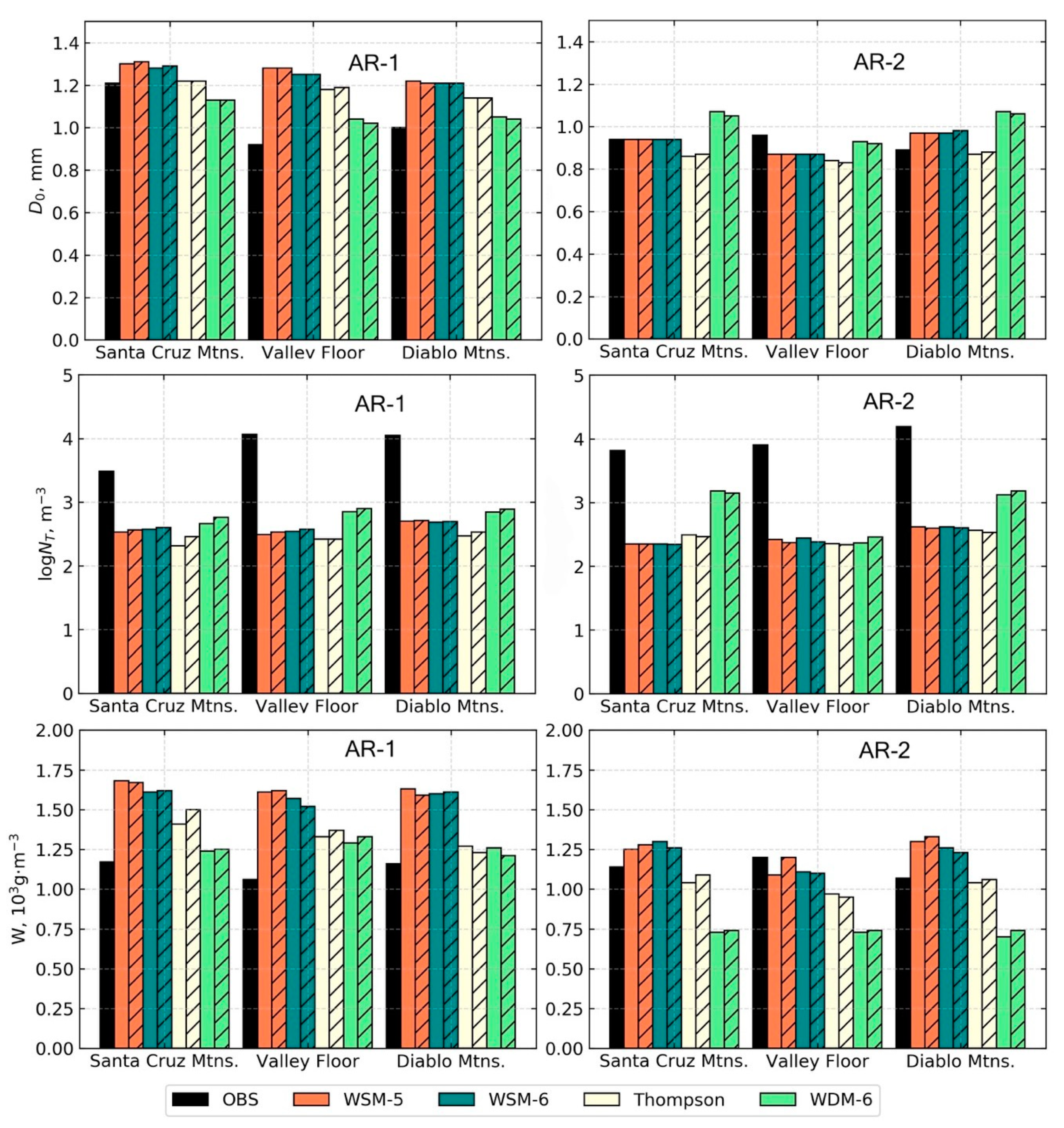
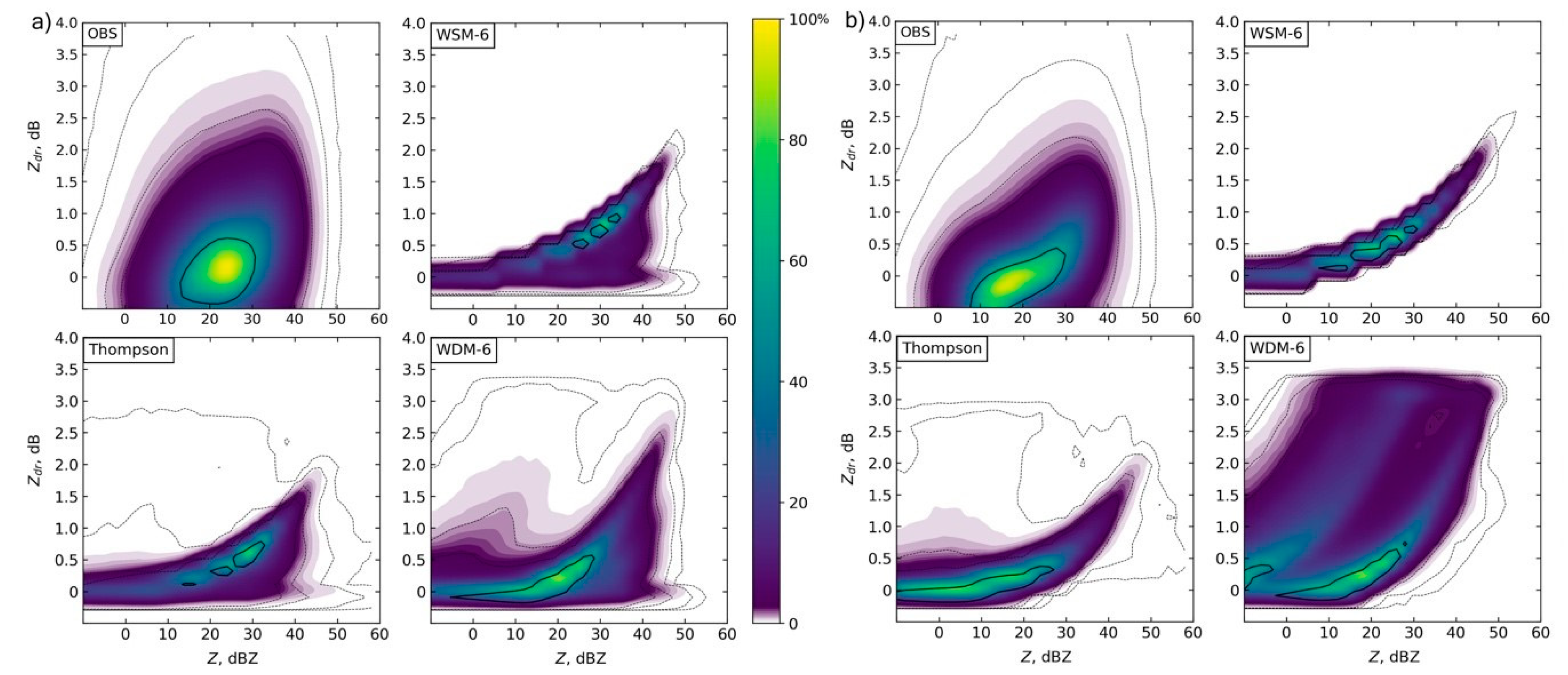
3.2. Simulated Radar and DSD
4. Conclusions and Remarks
Author Contributions
Acknowledgments
Conflicts of Interest
References
- Dettinger, M.D.; Ralph, F.M.; Das, T.; Neiman, P.J.; Cayan, D.R. Atmospheric Rivers, Floods and the Water Resources of California. Water 2011, 3, 445–478. [Google Scholar] [CrossRef]
- Ralph, F.M.; Dettinger, M.D. Historical and National Perspectives on Extreme West Coast Precipitation Associated with Atmospheric Rivers During December 2010. Bull. Am. Meteorol. Soc. 2012, 93, 783–790. [Google Scholar] [CrossRef]
- Guan, B.; Molotch, N.P.; Waliser, D.E.; Fetzer, E.J.; Neiman, P.J. Extreme snowfall events linked to atmospheric rivers and surface air temperature via satellite measurements. Geophys. Res. Lett. 2010, 37, L20401. [Google Scholar] [CrossRef]
- Ralph, F.M.; Dettinger, M.D. Storms, Floods, and the Science of Atmospheric Rivers. EOS Trans. AGU 2011, 92, 265–266. [Google Scholar] [CrossRef]
- Ralph, F.M.; Coleman, T.; Neiman, P.J.; Zamora, R.J.; Dettinger, M.D. Observed Impacts of Duration and Seasonality of Atmospheric-River Landfalls on Soil Moisture and Runoff in Coastal Northern California. J. Hydrometeorol. 2013, 14, 443–459. [Google Scholar] [CrossRef]
- Ralph, F.M.; Neiman, P.J.; Kingsmill, D.E.; Persson, P.O.G.; White, A.B.; Strem, E.T.; Andrews, E.D.; Antweiler, R.C. The Impact of a Prominent Rain Shadow on Flooding in California’s Santa Cruz Mountains: A CALJET Case Study and Sensitivity to the ENSO Cycle. J. Hydrometeorol. 2003, 4, 1243–1264. [Google Scholar] [CrossRef]
- Martner, B.E.; Yuter, S.E.; White, A.B.; Matrosov, S.Y.; Kingsmill, D.E.; Ralph, F.M. Raindrop Size Distributions and Rain Characteristics in California Coastal Rainfall for Periods with and without a Radar Bright Band. J. Hydrometeorol. 2008, 9, 408–425. [Google Scholar] [CrossRef]
- Hong, S.; Dudhia, J.; Chen, S. A Revised Approach to Ice Microphysical Processes for the Bulk Parameterization of Clouds and Precipitation. Mon. Weather Rev. 2004, 132, 103–120. [Google Scholar] [CrossRef]
- Igel, A.L.; Igel, M.R.; van den Heever, S.C. Make It a Double? Sobering Results from Simulations Using Single-Moment Microphysics Schemes. J. Atmos. Sci. 2015, 72, 910–925. [Google Scholar] [CrossRef]
- Hong, S.-Y.; Lim, J.-O.J. The WRF Single-Moment 6-Class Microphysics Scheme (WSM-6). J. Korean Metorol. Soc. 2006, 42, 129–151. [Google Scholar]
- Thompson, G.; Field, P.R.; Rasmussen, R.M.; Hall, W.D. Explicit Forecasts of Winter Precipitation Using an Improved Bulk Microphysics Scheme. Part II: Implementation of a New Snow Parameterization. Mon. Weather Rev. 2008, 136, 5095–5115. [Google Scholar] [CrossRef]
- Lim, K.-S.S.; Hong, S. Development of an Effective Double-Moment Cloud Microphysics Scheme with Prognostic Cloud Condensation Nuclei (CCN) for Weather and Climate Models. Mon. Weather Rev. 2010, 138, 1587–1612. [Google Scholar] [CrossRef]
- Mlawer, E.J.; Taubman, S.J.; Brown, P.D.; Iacono, M.J.; Clough, S.A. Radiative transfer for inhomogeneous atmospheres: RRTM, a validated correlated-k model for the longwave. J. Geophys. Res. Atmos. 1997, 102, 16663–16682. [Google Scholar] [CrossRef]
- Dudhia, J. Numerical Study of Convection Observed during the Winter Monsoon Experiment Using a Mesoscale Two-Dimensional Model. J. Atmos. Sci. 1989, 46, 3077–3107. [Google Scholar] [CrossRef]
- Niu, G.Y.; Yang, Z.L.; Mitchell, K.E.; Chen, F.; Ek, M.B.; Barlage, M.; Kumar, A.; Manning, K.; Niyogi, D.; Rosero, E.; et al. The community Noah land surface model with multiparameterization options (Noah-MP): 1. Model description and evaluation with local-scale measurements. J. Geophys. Res. Atmos. 2011, 116, D12109. [Google Scholar] [CrossRef]
- Jiménez, P.A.; Dudhia, J.; González-Rouco, J.F.; Navarro, J.; Montávez, J.P.; García-Bustamante, E. A Revised Scheme for the WRF Surface Layer Formulation. Mon. Weather Rev. 2012, 140, 898–918. [Google Scholar] [CrossRef]
- Hong, S.-Y.; Noh, Y.; Dudhia, J. A New Vertical Diffusion Package with an Explicit Treatment of Entrainment Processes. Mon. Weather Rev. 2006, 134, 2318–2341. [Google Scholar] [CrossRef]
- Efstathiou, G.A.; Zoumakis, N.M.; Melas, D.; Lolis, C.J.; Kassomenos, P. Sensitivity of WRF to boundary layer parameterizations in simulating a heavy rainfall event using different microphysical schemes. Effect on large-scale processes. Atmos. Res. 2013, 132–133, 125–143. [Google Scholar] [CrossRef]
- Houze, R.A. Orographic Effects on Precipitating Clouds. Rev. Geophys. 2012, 50, RG1001. [Google Scholar] [CrossRef]
- Bryan, G.H.; Morrison, H. Sensitivity of a Simulated Squall Line to Horizontal Resolution and Parameterization of Microphysics. Mon. Weather Rev. 2012, 140, 202–225. [Google Scholar] [CrossRef]
- Kovačević, N.; Ćurić, M. Precipitation sensitivity to the mean radius of drop spectra: Comparison of single and double-moment bulk microphysical schemes. Atmosphere 2015, 6, 451–473. [Google Scholar] [CrossRef]
- Brown, B.R.; Bell, M.M.; Frambach, A.J. Validation of simulated hurricane drop size distributions using polarimetric radar. Geophys. Res. Lett. 2016, 43, 910–917. [Google Scholar] [CrossRef]
- Leinonen, J. High-level interface to T-matrix scattering calculations: Architecture, capabilities and limitations. Opt. Express 2014, 22, 1655–1660. [Google Scholar] [CrossRef] [PubMed]
- Cunningham, J.G.; Zittel, W.D.; Lee, R.R.; Ice, R.L.; Hoban, N.P. Methods for Identifying Systematic Differential Reflectivity (Zdr) Biases on the Operational WSR-88D Network. In Proceedings of the 36th Conference on Radar Meteorology, Breckenridge, CO, USA, 16–20 September 2013; Volume 9, pp. 1–24. [Google Scholar]
- Ryzhkov, A.V.; Giangrande, S.E.; Melnikov, V.M.; Schuur, T.J. Calibration issues of dual-polarization radar measurements. J. Atmos. Ocean. Technol. 2005, 22, 1138–1155. [Google Scholar] [CrossRef]
- Brandes, E.A.; Zhang, G.; Vivekanandan, J. An Evaluation of a Drop Distribution–Based Polarimetric Radar Rainfall Estimator. J. Appl. Meteorol. 2003, 42, 652–660. [Google Scholar] [CrossRef]
- Brandes, E.A.; Zhang, G.; Vivekanandan, J.; Brandes, E.A.; Zhang, G.; Vivekanandan, J. Drop Size Distribution Retrieval with Polarimetric Radar: Model and Application. J. Appl. Meteorol. 2004, 43, 461–475. [Google Scholar] [CrossRef]
- Zhang, J.; Howard, K.; Langston, C.; Kaney, B.; Qi, Y.; Tang, L.; Grams, H.; Wang, Y.; Cockcks, S.; Martinaitis, S.; et al. Multi-Radar Multi-Sensor (MRMS) quantitative precipitation estimation: Initial operating capabilities. Bull. Am. Meteorol. Soc. 2016, 97, 621–638. [Google Scholar] [CrossRef]
- Qi, Y.; Martinaitis, S.; Zhang, J.; Cocks, S. A Real-Time Automated Quality Control of Hourly Rain Gauge Data Based on Multiple Sensors in MRMS System. J. Hydrometeorol. 2016, 17, 1675–1691. [Google Scholar] [CrossRef]
- Neiman, P.J.; Ralph, F.M.; Wick, G.A.; Lundquist, J.D.; Dettinger, M.D. Meteorological Characteristics and Overland Precipitation Impacts of Atmospheric Rivers Affecting the West Coast of North America Based on Eight Years of SSM/I Satellite Observations. J. Hydrometeorol. 2008, 9, 22–47. [Google Scholar] [CrossRef]
- Ralph, F.M.; Dettinger, M.; Cordeira, J.M.; Rutz, J.J.; Schick, L.; Anderson, M.; Smallcomb, C.; Reynolds, D. A Scale to Characterize the Strength and Impacts of Atmospheric Rivers. Bull. Am. Meteorol. Soc. 2019. [Google Scholar] [CrossRef]
- Neiman, P.J.; White, A.B.; Ralph, F.M.; Gottas, D.J.; Gutman, S.I. A water vapour flux tool for precipitation forecasting. Proc. Inst. Civ. Eng. Water Manag. 2009, 162, 83–94. [Google Scholar] [CrossRef]
- Cifelli, R.; Chandrasekar, V.; Chen, H.; Johnson, L.E. High Resolution Radar Quantitative Precipitation Estimation in the San Francisco Bay Area: Rainfall Monitoring for the Urban Environment. J. Meteorol. Soc. Jpn. 2018, 96, 141–155. [Google Scholar] [CrossRef]
- Matrosov, S.Y.; Cifelli, R.; Neiman, P.J.; White, A.B. Radar rain-rate estimators and their variability due to rainfall type: An assessment based on hydrometeorology testbed data from the southeastern United States. J. Appl. Meteorol. Clim. 2016, 55, 1345–1358. [Google Scholar] [CrossRef]


| WSM-5 | WSM-6 | Thompson | WDM-6 |
|---|---|---|---|
| Cloud | Cloud | Cloud | Cloud * |
| Ice | Ice | Ice * | Ice |
| Rain | Rain | Rain * | Rain * |
| Snow | Snow | Snow | Snow |
| Water vapor | Water vapor | Water vapor | Water vapor |
| - | Graupel | Graupel | Graupel |
| - | - | - | CCN † |
| Bias Correction | November 16 | April 6 |
|---|---|---|
| WSR-88D Internal | −0.179 dB | −0.198 dB |
| Rhyzkov Light rain | −0.161 dB | −0.241 dB |
© 2019 by the authors. Licensee MDPI, Basel, Switzerland. This article is an open access article distributed under the terms and conditions of the Creative Commons Attribution (CC BY) license (http://creativecommons.org/licenses/by/4.0/).
Share and Cite
Behringer, D.; Chiao, S. Numerical Investigations of Atmospheric Rivers and the Rain Shadow over the Santa Clara Valley. Atmosphere 2019, 10, 114. https://doi.org/10.3390/atmos10030114
Behringer D, Chiao S. Numerical Investigations of Atmospheric Rivers and the Rain Shadow over the Santa Clara Valley. Atmosphere. 2019; 10(3):114. https://doi.org/10.3390/atmos10030114
Chicago/Turabian StyleBehringer, Dalton, and Sen Chiao. 2019. "Numerical Investigations of Atmospheric Rivers and the Rain Shadow over the Santa Clara Valley" Atmosphere 10, no. 3: 114. https://doi.org/10.3390/atmos10030114
APA StyleBehringer, D., & Chiao, S. (2019). Numerical Investigations of Atmospheric Rivers and the Rain Shadow over the Santa Clara Valley. Atmosphere, 10(3), 114. https://doi.org/10.3390/atmos10030114