Article

Algorithm for Improved QPE over Complex Terrain Using Cloud-to-Ground Lightning Occurrences

by
Carlos Minjarez-Sosa
1,*,
Julio Waissman
2,
Christopher L. Castro
3 and
David Adams
4
1
Departamento de Física, Universidad de Sonora, Hermosillo, Son 83000, Mexico
2
Departamento de Matemátcas, Universidad de Sonora, Hermosillo, Son 83000, Mexico
3
Hydrology and Atmospheric Sciences Department, University of Arizona, Tucson, AZ 85721, USA
4
Centro de Ciencias de la Atmósfera, UNAM, Ciudad de México 04510, Mexico
*
Author to whom correspondence should be addressed.
Atmosphere 2019, 10(2), 85; https://doi.org/10.3390/atmos10020085
Submission received: 17 January 2019 / Revised: 7 February 2019 / Accepted: 11 February 2019 / Published: 19 February 2019
(This article belongs to the Section Meteorology)

Abstract

:
Lightning and deep convective precipitation have long been studied as closely linked variables, the former being viewed as a proxy, or estimator, of the latter. However, to date, no single methodology or algorithm exists for estimating lightning-derived precipitation in a gridded form. This paper, the third in a series, details the specific algorithm where convective rainfall was estimated with cloud-to-ground lightning occurrences from the U.S. National Lightning Detection Network (NLDN), for the North American Monsoon region. Specifically, the authors present the methodology employed in their previous studies to get this estimation, noise test, spatial and temporal neighbors and the algorithm of the Kalman filter for dynamically derived precipitation from lightning.

1. Introduction

Precipitation is one of the most important elements of the atmospheric hydrological cycle as well as the climate system [1,2]. Precipitation must be accurately measured over a large range of spatio-temporal scales, for example, from convective storms to the global climate system as well as provide accurate measures for applications to water resources, agriculture and civil protection [1,3,4,5,6]. On the larger end of the scale (continental to planetary), Quantitative Precipitation Estimation (QPE) is necessary for accurate assessement of the atmospheric energy budget and hydrological cycle [7]. On higher space and time scales, it is also a key component in short-term forecasts (nowcasting) of flooding and other extreme weather events (e.g., [4,5]).
However, due to its high spatio-temporal variability, precipitation is one of the most difficult variables to monitor [8]. Rain gauges, under ideal conditions, are considered the most accurate point measurement of precipitation; however, for estimating QPE, geo-statistical methods are necessary and the accuracy of the estimation depends on gauge network density, which in most cases is not adequate [9,10,11,12]. Weather radars, on the other hand, are characterized as having high spatio-temporal resolution and coverage and have been considered the best operational option for estimation of rainfall [5,13,14]. Radars, nevertheless, also have limitations, such as poor coverage in mountainous regions, no unique Z-R relationship, and evaporation of rain from higher altitudes, among others [5,14,15,16].
In light of the fact that each of these techniques has limitations for QPE estimation, some researchers have offered merged products, for example, rain gauges and weather radar data [17,18,19,20] to generate gridded QPE. To these data, others have added climatologies of orographic precipitation [21] to produce a multi-sensor QPE (MQPE) and improve QPE accuracy. However, even with this combination of all these data sources and error reduction methodologies, precipitation estimation still suffers from problems with accuracy in regions with complex terrain [21,22,23].
In the last three decades, other techniques, such as satellite-derived precipitation, have been proposed and incorporated for QPE. Satellite-derived precipitation is not limited by coverage problems in mountainous regions as radars are, but it has its deficiencies [23]. Mehran and AghaKouchak [24], in comparing satellite QPE with products like PERSIANN [25], CMORPH [26], and TRMM Multi-Satellite Precipitation Analysis Real Time (TMPA-RT) [27] revealed errors for strong precipitation events associated with topography; that is, precisely where multi-sensor methods also produce inaccuracies. Another limitation is that, at least for quantitative precipitation forecasting (QPF), its temporal resolution and latency (which is about 15 min) make these products useful for short-term QPF [28], but not for better precipitation nowcasts. Even with existing modern techniques and methods for QPE, the problems with precipitation estimation persist, especially in regions with poor sensor coverage such as mountainous terrain [22,23,24] where rainfall can be more frequent and copious.

1.1. Lightning-Precipitation Relationship (LPR)

Since the mid-twentieth century, many authors have proposed lightning as an estimator of precipitation. Workman and Reynolds [29] reported on the relationship between cloud electrical activity and precipitation. Battan [30] later calculated a rain-yield per flash by visually counting cloud-to-ground (CG) lightning events in southern Arizona. A number of studies such as [31,32,33,34,35]; among many others, have shown that lightning can be used as an estimator of convective precipitation (for a more extended review of these studies please see [36]). Research findings show that the lightning-precipitation relationship varies over a wide range of scales; temporal (minutes to seasonal) and spatial (storm scale, e.g., [34]) to complete regions (about 104 km 2 ; e.g., [33]).

1.2. Summary of Previous Work

This study is the third in a series of three papers examining LPR to estimate QPE. In the first paper, Minjarez and co-authors [22] investigated the relationship between convective precipitation and cloud-to-ground lightning in southwest Arizona and northern Sonora, Mexico employing STAGE IV NCEP data for the summer of 2005. The authors developed a LPR-based QPE method for seasonal, daily and hourly precipitation estimation in regions with poor sensor coverage, as well as a method to spatially smooth discrete lightning counts to estimate convective rainfall thereby improving quality and spatial coverage of radar-derived precipitation estimation. The effect of using poor sensor coverage negatively affects LPR, when non-covered regions were included, which is revealed in the decrease in explained variance R 2 between CG lightning and precipitation from 0.39 to 0.23. Finally, by using 1-h accumulated lightning data, the study estimated convective precipitation, finding that about 67% of total precipitation for the 2005 season can be related with CG lightning. Their method was successful in tracking air mass storms and more complex multicellular convective systems in regions with poor sensor coverage.
In [23], the authors improved their methodology for QPE estimation by using lightning at a space and time resolution of 5 km and 5 min. In order to address the time and space displacement that occurs when LPR is correlated at high resolutions, a linear space and time-invariant model was developed, leading to improved results in comparison to the two parameter model in the 2012 study. An optimal time and space neighboring for the gridded data that considered four time lags and one future time step and two coincident spatial neighbors was obtained. Since this linear model is fixed, the time variation in LPR that may occur within a storm was addressed by applying a time variant Kalman filter, which significantly improved the fixed time model.
Performing a data denial analysis in a radar-covered region, this study also provided more and stronger evidence that in a region with proper precipitation sensor coverage, like western Texas, the model can be calibrated by using the covered grids and precipitation can then be estimated in grids with poor sensor coverage.
With the aim of contributing to the development and promoting the use of lightning for estimating precipitation, this article presents, in detail, the algorithm developed by Minjarez and co-authors [23] to estimate QPE by cloud-to-ground lightning, as well as the methodology developed to test the model and select the parameters that were employed in the 2017 study.

2. Materials and Methods
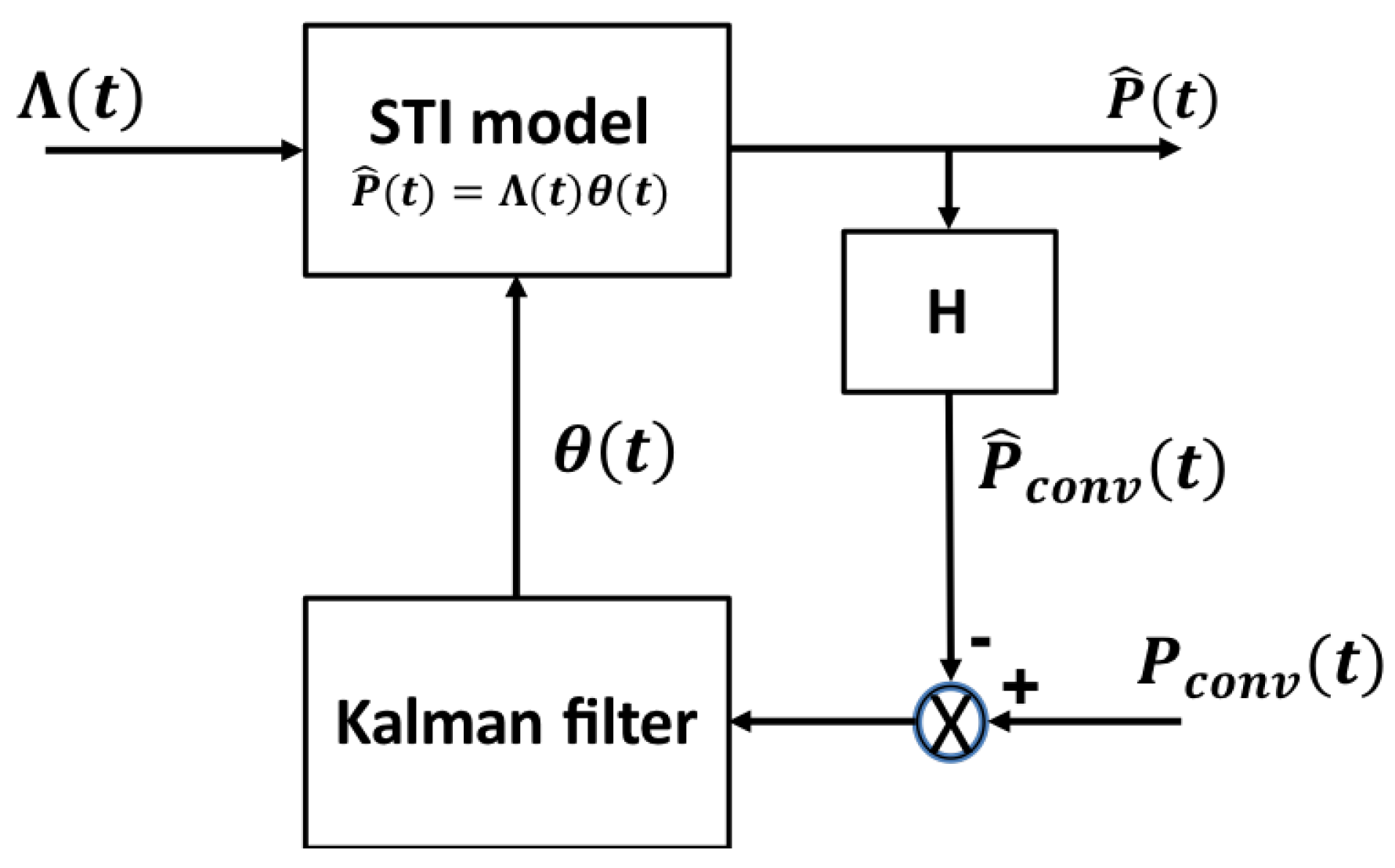
Here, we present a linear multispatial-temporal model for estimating precipitation from cloud-to-ground lightning counts. In general, linearly estimated precipitation at time t and the ( i , j ) grid can be defined as:
P ^ i , j = f i , j ( L , t ) T , 1 T θ
where f i , j ( L , t ) = [ f i , j 1 ( L , t ) , , f i , j k ( L , t ) ] is a feature vector of dimension k at time t from lightning observations L, and θ = [ θ 1 , , θ k , b ] is a vector of estimation parameters.
For example, in [22], a model is developed by comparing the mean of convective precipitation in the sensor-covered domain at every time step with the corresponding lightning flash sum in the same domain. For this case f i , j ( L , t ) = L i , j ( t ) is established with only one feature as
f i , j ( L , t ) = [ L i , j ( t ) ]
where L i , j ( t ) are the Gaussian lightning counts at time t and ( i , j ) grid. Thus, the model is
P ^ i , j = L i , j ( t ) , 1 T θ
P ^ i , j = θ L i , j ( t ) + b
The model parameters θ and b can be estimated in two ways. First, in order to calculate the model parameters, a vector of the mean of precipitation and lightning are calculated as:
L ¯ ( t ) = 1 N ( t ) i , j L i , j ( t ) ,
P ¯ ( t ) = 1 N ( t ) i , j P i , j ( t ) ,
where N ( t ) is the number of grids with Gaussian counts different from zero at time t. The parameters are obtained by resolving the equation using least squares
P ¯ ( t ) = θ L ¯ ( t ) + b .
The model parameters are calculated by comparing the total seasonal convective precipitation (as defined by [23]) accumulation with the total lightning accumulated per grid.
Next, we describe the linear model with spatial and time neighbors, denominated [23] the Spatial and Time Invariant (STI) Model, or seasonal model. Let N b V represent the spatial neighboring of the grid i , j at time t with V spatial neighbors in the vicinity:
N b V ( L i , j ( t ) ) = [ L i V , j V ( t ) , , L i , j ( t ) , , L i V , j V ( t ) ] T ,
Let Λ i , j ( t ) be the temporally associated vector of lightning observations
Λ i , j ( t ) = N b V ( L i , j ( t I N ) ) T , , N b V ( L i , j ( t ) ) T , , N b V ( L i , j ( t + I P ) ) T , 1 ,
where I N are the previous time steps (negative time lags) and I P are the latter time steps (positive time lags). Λ i j ( t ) is a row vector that contains the Gaussian lightning counts of the grid i , j and its neighbors for each time lag considered in the STI model.
The STI model can now be described as:
P ^ i , j ( t ) = Λ ( t ) θ
and θ = ( θ 1 , , θ k , b ) is the model parameter vector, where k = ( 2 V + 1 ) 2 · ( I P + I N + 1 ) . The vector θ is adjusted by a least squares criteria by using the grids where is determined that convection is occurring in the relevant dataset.
A static STI model, fixed over all times, is most certainly not a very robust assumption. The model can substantially vary from one convective event to another and even during the evolution of the storm and this is not accounted for by the STI model. A more realistic model would dynamically respond to slowly varying LPR changes in time. In this respect, one of the methods that has been widely used for data assimilation in the atmospheric sciences, particularly for precipitation estimation, is the Kalman filter [37,38]. In its original form, the Kalman filter is a linear recursive algorithm that minimizes the mean-squared error to estimate the state of a process. Use of the Kalman filter is thus a straightforward and efficient solution for constructing a time-varying LPR.
The basic idea is to consider the vector parameter θ as a discrete dynamical system of the form
θ ( t ) = θ ( t 1 ) + W ( t ) ,
where W ( t ) is a parameter estimation error, modeled as a Gaussian random vector with zero mean and a covariance matrix Q. The estimation algorithm is then used to minimize the error between the observed precipitation at time t and the estimated precipitation obtained with the model and the parameter vector θ . The typical use for a Kalman filter is using a known system and observation operator to estimate the system’s state given noisy observations. In our approach the Kalman filter is used in a different way, namely to update the system itself, similar to the one used by [39].
In order to employ Kalman filter, the estimated precipitation for the whole dataset at time t is calculated as:
P ^ ( t ) = Λ 0 , 0 ( t ) Λ N , M ( t ) θ = Λ ( t ) θ ,
where N is the number of rows and M is the number of columns of grids that define the Cartesian regions to be analyzed and is the estimated precipitation vector.
However, θ estimation should be realized only with covered grids (grids with valid precipitation observations). Then, let Y ( t ) = ( Y 1 ( t ) , , Y C ( t ) ) + V ( t ) be the observed precipitation vector at time t for just the covered grids and V ( t ) is the observation noise, assumed Gaussian with zero mean and covariance R. The estimated precipitation of covered grids is assumed, similar to the STI model, to be:
Y ^ ( t ) = H Λ ( t ) θ ,
where H is a matrix of dimension ( C , N × M ) . Entries H a , b = 1 if Y a ( t ) correspond to the jth element of the vector P ( t ) , else H i j = 0 . H is then a matrix used to reduce a vector of dimension N × M that represents the observed precipitation as a vector with only the covered grids.
Figure 1 shows the scheme of the procedure. The Kalman filter algorithm steps performed for each new time-step t are:
  • Update the error matrix E ( t ) and the covariance matrix A ¯ ( t )
    A ¯ ( t ) = Λ ( t ) A ( t 1 ) Λ T ( t ) + Q
    E ( t ) = Y ( t ) H Λ ( t ) θ ( t 1 )
  • Update the Kalman gain matrix K ( t )
    Z ( t ) = H Λ ( t )
    K ( t ) = A ¯ Z T ( t ) Z ( t ) A ¯ Z T ( t ) + R 1
  • Update the model parameter vector estimation θ ( t )
    θ ( t ) = θ ( t 1 ) + K ( t ) E ( t )
  • Prepare covariance A ( t ) for the next time-step
    A ( t ) = I K ( t ) Z ( t ) A ¯ ( t )
  • Produce updated precipitation estimate P ^ ( t )
    P ^ ( t ) = Λ ( t ) θ ( t )
    where A ( t ) is the a posteriori error covariance matrix. In order to apply the Kalman filter there is a need to impose an initial condition A ( 0 ) and the covariance matrix Q and R. The value of A ( 0 ) determines the initial estimation rate of the Kalman filter and is normally used as a diagonal matrix with large values.
In our implementation of the algorithm, we initiate the Kalman filter with the STI model parameters derived from long-term observations. Once the Kalman estimation commences, it dynamically adjusts the coefficients at each time step (5 min) until 5 consecutive time steps report no lightning in the covered domain. At this point, the coefficients slowly (5 time steps) revert back to those of the STI which can be viewed as the best guess in the absence of new information. The rate at which we revert back is based loosely on the time evolution of a typical thunderstorm (air mass type) which lasts about 45–60 min, including developing, mature, and decay phases. Thus, we assert that our time lags assumption (25 min) is sufficiently long to assure that the next lightning strike will be associated with a new cell/storm. Although somewhat arbitrary, this period is certainly consistent with the physics of the problem.

3. Results

3.1. Time and Space Neighboring

A novel way to treat the time and space misplacement in LPR is to use neighbors for higher resolutions. Figure 2 compares the correlation (vertical axes) for several time lags (horizontal axes) and space neighboring situations. It shows the variation in correlation coefficients between STI estimated and observed precipitation, considering all 10 lags and 4 space neighbor scenarios.
The results from Figure 2 show that, at high space and time resolutions, if precipitation and lightning at grid i , j are correlated without space and time neighbors, the relationship results are poor (between 0.1 and 0.25 for this case). This model can work for larger spatio-temporal resolutions, as shown by [22], for the seasonal case and 8 km grid size. By observing and evaluating the correlation plots, the benefit that results from the time and space neighbors is evident, although this varies from season to season and from region to region.
For instance, for the southern Arizona area, comparing the correlation with and without use of spatial neighboring, the maximum benefit from the spatial neighbors is (over an average of 2 years) ∼16%, practically the same as the Texas result, a totally sensor covered region. The use of time lags has a maximum average impact of ∼20% for both regions. With just the addition of one past lag (000110000 lag scenario) the correlation increases up to 13% in comparison with 0-lag scenario.
If we compare this with the increment in correlation for the time lag case 000111000 (one future and one past time lags), we find that the past time lags are more relevant than the future ones. The impact on the correlation of using all time lags with respect to using past and one future lag is not more than 3% for both sites and for both seasons. Given the negligible computational benefit, this last lag criteria was chosen for our study.
This last result can be used as the threshold to differentiate the benefit from the improvement of the physics of the LPR and the mathematical benefit of only having more model parameters. The time neighboring more or less matches with the times reported by other authors where precipitation and CG lightning are correlated [34,35,40]. In the combination of time lags and space neighbors there were no significant differences (regarding the 3% referred in the last paragraph) for more than 2 space neighbors. For grid spacing of about 5 km, representing an area of 25 square km, this suggests that at least one propagating air mass thunderstorm with its convective core and some of the transient stratiform precipitation can be captured.

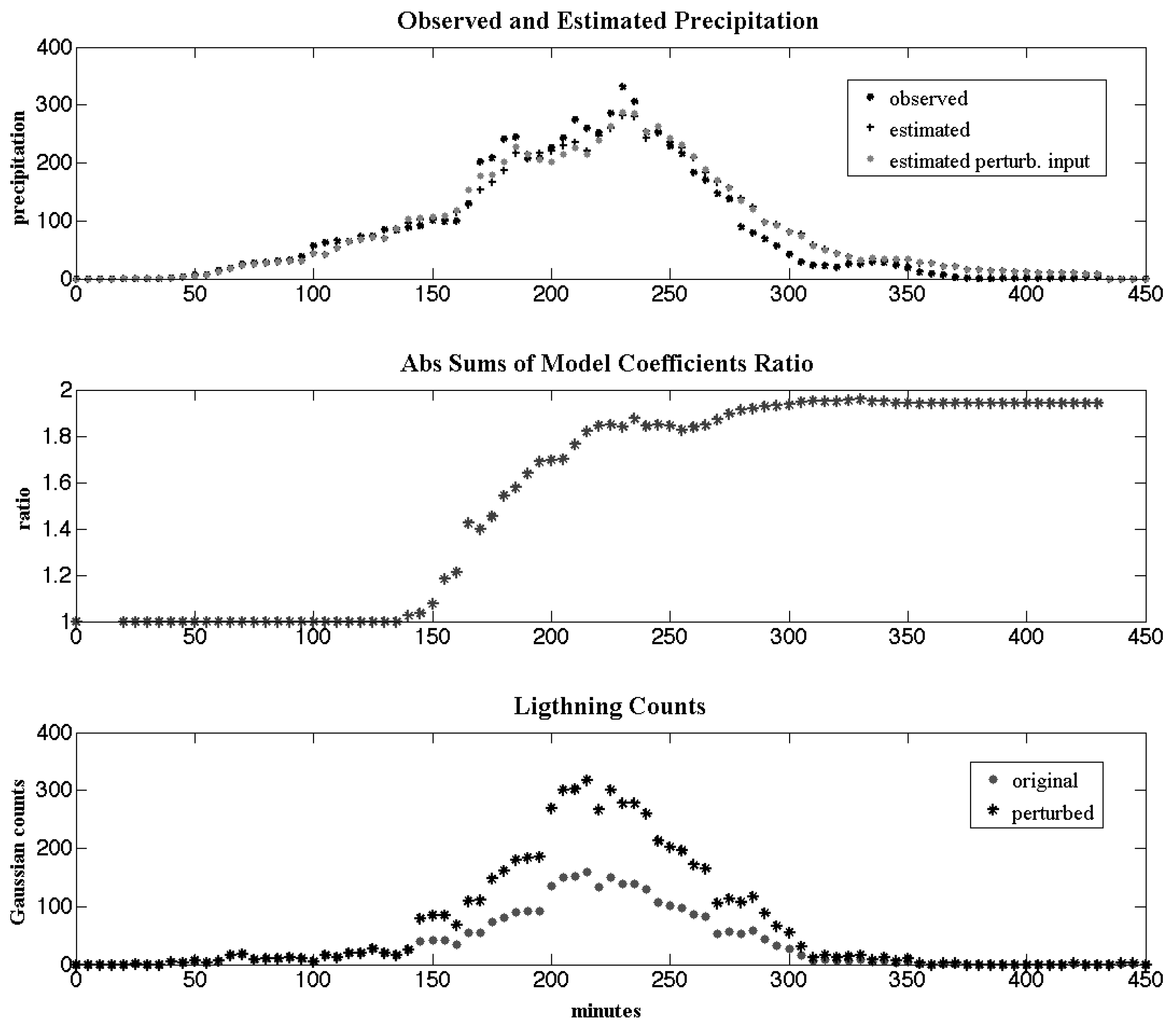
3.2. Kalman Filter Testing Model Robustness

Overall, one of the factors that must be considered for a Kalman filter is the sensitivity to noise and model errors. In general, a robust model that does not track the high frequency variations in the Kalman error ( E ( t ) above) is required.
For this study, a test of model robustness was performed. This test consisted of running the Kalman filter using real lightning observations as input, but scaled up by 2, starting at a specific point in time (shown in the top panel of Figure 3 below). It is expected that with the appropriate parameters in the correlation matrixes R and Q, this division will cause the Kalman filter to smoothly reduce the sum of the filter coefficients by a factor of 2 (after some time steps).
Early attempts at this analysis found that the absence of persistent, excitation of the Kalman filter (few or no lightning input) can affect this testing, so Gaussian noise was added to the input in order to have all temporal values different to zero. Figure 3 shows a panel with the steps of this test for the event at the Texas site for the 150th day of 2009. The top plot shows Gaussian counts time series, the middle panel shows the ratio for the total parameter sum and, at the bottom panel, the time series of P ^ per each lightning entry is presented.
Figure 3 shows disagreement between the P ^ from the scaled input with that of the true input once the lightning strikes are degraded at around minute 150. It is clear that the parameters slowly adjust themselves to compensate for this “step” change in input, and when the ratio converges to 2 the estimated precipitation converge for both conditions (estimated from degraded input and another). This demonstrates that the selected Kalman parameters are appropriate for our use.

4. Discussion

In this article, the details of the methodology for estimating precipitation through use of cloud-to-ground lightning occurrences was presented. A linear model was developed for this purpose, spatial and time neighbors were used as a static filter which initiates the Kalman filter. A study of what was the optimal space and time neighboring was performed obtaining that the relation cost-benefit in terms of correlation and computational cost was 2 space and 5 time neighbors. As stated in [23]; this neighbor configuration provides better results, in general, for the season and individual convective storms in Texas and Arizona.
As presented, we intend for this methodology to be used as a new precipitation estimator which can also be integrated to the other techniques for calculating QPE, especially, but not exclusively for, those areas of strong convective precipitation and poor sensor coverage (e.g., southern Arizona). Finally, it should be clearly stated that this methodology just estimates convective precipitation associated or explained by lightning (as [22,23] defined) and thus does not estimate stratiform precipitation. This is one weaknesses of this method. Given that some authors have pointed out that current multi-sensor products still miss some strong convective events [24,41], our lightning-derived precipitation methodology can be utilized as another source of estimation for precisely these convective events and, hence, integrated as another source of Muli-sensor derived precipitation.

Author Contributions

Conceptualization, C.M.-S. and J.W.; Formal analysis, C.M.-S.; Funding acquisition, C.M.-S.; Investigation, C.M.-S.; Methodology, C.M.-S., J.W., C.L.C. and D.A.; Software, C.M.-S. and J.W.; Supervision, J.W. and C.L.C.; Validation, C.M.-S.; Visualization, C.M.-S.; Writing—original draft, C.M.-S.; Writing—review & editing, C.L.C. and D.A.

Funding

This work was supported by CONACYT project Fellowship 187242, The University of Arizona through Graduate Incentives for Growth Award (GIGA) Fellowship and Vaisala Inc.

Acknowledgments

We thank NSSL staff; in particular Ken Howard, Carrie Langstone and Jian Zhang for providing, and giving advice on, the NMQ precipitation data. We also thank Ken Cummins for all his advice and guidance in this research.

Conflicts of Interest

The authors declare no conflict of interest. The funders had no role in the design of the study; in the collection, analyses, or interpretation of data; in the writing of the manuscript, or in the decision to publish the results.

References

  1. Adam, J.C.; Lettenmaier, D.P. Adjustment of global gridded precipitation for systematic bias. J. Geophys. Res. Atmos. 2003, 108. [Google Scholar] [CrossRef] [Green Version]
  2. Yang, B.; Qin, C.; Wang, J.; He, M.; Melvin, T.M.; Osborn, T.J.; Briffa, K.R. A 3500-year tree-ring record of annual precipitation on the northeastern Tibetan Plateau. Proc. Natl. Acad. Sci. USA 2014, 111, 2903–2908. [Google Scholar] [CrossRef]
  3. Grecu, M.; Krajewski, W. A large-sample investigation of statistical procedures for radar-based short-term quantitative precipitation forecasting. J. Hydrol. 2000, 239, 69–84. [Google Scholar] [CrossRef]
  4. Todd, M.C.; Kidd, C.; Kniveton, D.; Bellerby, T.J. A combined satellite infrared and passive microwave technique for estimation of small-scale rainfall. J. Atmos. Ocean. Technol. 2001, 18, 742–755. [Google Scholar] [CrossRef]
  5. Krajewski, W.; Smith, J. Radar hydrology: Rainfall estimation. Adv. Water Resour. 2002, 25, 1387–1394. [Google Scholar] [CrossRef]
  6. Bauer, P.; Thorpe, A.; Brunet, G. The quiet revolution of numerical weather prediction. Nature 2015, 525, 47. [Google Scholar] [CrossRef]
  7. Sorooshian, S.; Lawford, R.; Try, P.; Rossow, W.; Roads, J.; Polcher, J.; Sommeria, G.; Schiffer, R. Water and energy cycles: Investigating the links. World Meteorol. Organ. Bull. 2005, 54, 58–64. [Google Scholar]
  8. Herrera, S.; Gutiérrez, J.M.; Ancell, R.; Pons, M.; Frías, M.; Fernández, J. Development and analysis of a 50-year high-resolution daily gridded precipitation dataset over Spain (Spain02). Int. J. Climatol. 2012, 32, 74–85. [Google Scholar] [CrossRef]
  9. Brandes, E.A.; Vivekanandan, J.; Wilson, J.W. A comparison of radar reflectivity estimates of rainfall from collocated radars. J. Atmos. Ocean. Technol. 1999, 16, 1264–1272. [Google Scholar] [CrossRef]
  10. Habib, E.; Krajewski, W. Uncertainty analysis of the TRMM ground-validation radar-rainfall products: Application to the TEFLUN-B field campaign. J. Appl. Meteorol. 2002, 41. [Google Scholar] [CrossRef]
  11. Morin, E.; Gabella, M. Radar-based quantitative precipitation estimation over Mediterranean and dry climate regimes. J. Geophys. Res. Atmos. 2007, 112. [Google Scholar] [CrossRef] [Green Version]
  12. Villarini, G.; Mandapaka, P.V.; Krajewski, W.F.; Moore, R.J. Rainfall and sampling uncertainties: A rain gauge perspective. J. Geophys. Res. Atmos. 2008, 113. [Google Scholar] [CrossRef] [Green Version]
  13. Doswell, C.A., III; Brooks, H.E.; Maddox, R.A. Flash flood forecasting: An ingredients-based methodology. Weather Forecast. 1996, 11, 560–581. [Google Scholar] [CrossRef]
  14. Morin, E.; Maddox, R.A.; Goodrich, D.C.; Sorooshian, S. Radar Z–R relationship for summer monsoon storms in Arizona. Weather Forecast. 2005, 20, 672–679. [Google Scholar] [CrossRef]
  15. Crosson, W.L.; Duchon, C.E.; Raghavan, R.; Goodman, S.J. Assessment of rainfall estimates using a standard ZR relationship and the probability matching method applied to composite radar data in central Florida. J. Appl. Meteorol. 1996, 35, 1203–1219. [Google Scholar] [CrossRef]
  16. Fulton, R.A. Sensitivity of WSR-88D rainfall estimates to the rain-rate threshold and rain gauge adjustment: A flash flood case study. Weather Forecast. 1999, 14, 604–624. [Google Scholar] [CrossRef]
  17. Stellman, K.M.; Fuelberg, H.E.; Garza, R.; Mullusky, M. An examination of radar and rain gauge–derived mean areal precipitation over Georgia watersheds. Weather Forecast. 2001, 16, 133–144. [Google Scholar] [CrossRef]
  18. Xie, P.; Arkin, P.A. An intercomparison of gauge observations and satellite estimates of monthly precipitation. J. Appl. Meteorol. 1995, 34, 1143–1160. [Google Scholar] [CrossRef]
  19. Kursinski, A.L.; Zeng, X. Areal estimation of intensity and frequency of summertime precipitation over a midlatitude region. Geophys. Res. Lett. 2006, 33. [Google Scholar] [CrossRef] [Green Version]
  20. Kitzmiller, D.; Miller, D.; Fulton, R.; Ding, F. Radar and multisensor precipitation estimation techniques in National Weather Service hydrologic operations. J. Hydrol. Eng. 2013, 18, 133–142. [Google Scholar] [CrossRef]
  21. Zhang, J.; Qi, Y.; Langston, C.; Kaney, B.; Howard, K. A real-time algorithm for merging radar QPEs with rain gauge observations and orographic precipitation climatology. J. Hydrometeorol. 2014, 15, 1794–1809. [Google Scholar] [CrossRef]
  22. Minjarez-Sosa, C.; Castro, C.L.; Cummins, K.L.; Krider, E.P.; Waissman, J. Improved QPE in complex terrain using cloud-toground lightning data: A case study for the 2005 monsoon in southern Arizona. J. Hydrometeorol. 2012, 13, 1855–1873. [Google Scholar] [CrossRef]
  23. Minjarez-Sosa, C.M.; Castro, C.L.; Cummins, K.L.; Waissman, J.; Adams, D.K. An improved QPE over complex terrain employing cloud-to-ground lightning occurrences. J. Appl. Meteorol. Climatol. 2017, 56, 2489–2507. [Google Scholar] [CrossRef]
  24. Mehran, A.; AghaKouchak, A.A. Capabilities of satellite precipitation datasets to estimate heavy precipitation rates at different temporal accumulations. Hydrol. Process. 2014, 28, 2262–2270. [Google Scholar] [CrossRef]
  25. Hsu, K.l.; Gao, X.; Sorooshian, S.; Gupta, H.V. Precipitation estimation from remotely sensed information using artificial neural networks. J. Appl. Meteorol. 1997, 36, 1176–1190. [Google Scholar] [CrossRef]
  26. Joyce, R.J.; Janowiak, J.E.; Arkin, P.A.; Xie, P. CMORPH: A method that produces global precipitation estimates from passive microwave and infrared data at high spatial and temporal resolution. J. Hydrometeorol. 2004, 5, 487–503. [Google Scholar] [CrossRef]
  27. Huffman, G.J.; Bolvin, D.T.; Nelkin, E.J.; Wolff, D.B.; Adler, R.F.; Gu, G.; Hong, Y.; Bowman, K.P.; Stocker, E.F. The TRMM multisatellite precipitation analysis (TMPA): Quasi-global, multiyear, combined-sensor precipitation estimates at fine scales. J. Hydrometeorol. 2007, 8, 38–55. [Google Scholar] [CrossRef]
  28. Zahraei, A.; Hsu, K.L.; Sorooshian, S.; Gourley, J.J.; Hong, Y.; Behrangi, A. Short-term quantitative precipitation forecasting using an object-based approach. J. Hydrol. 2013, 483, 1–15. [Google Scholar] [CrossRef]
  29. Workman, E.; Reynolds, S.; Byers, H. Structure and electrification. Thunderst. Electr. 1953, 139–149. [Google Scholar]
  30. Battan, L. Some factors governing precipitation and lightning from convective clouds. J. Atmos. Sci. 1965, 22, 79–85. [Google Scholar] [CrossRef]
  31. Piepgrass, M.; Krider, E.; Moore, C. Lightning and surface rainfall during florida thunderstorms. J. Geophys. Res. 1992, 87, 11195–11201. [Google Scholar] [CrossRef]
  32. Tapia, A.; Smith, J.; Dixon, M. Estimation of convective rainfall from lightning observations. Appl. Meteorol. 1998, 37, 1497–1509. [Google Scholar] [CrossRef]
  33. Petersen, W.; Rutledge, S. On the relationship between cloud-to-ground lightning and convective rainfall. Geophys. Res. 1998, 103, 14025–14040. [Google Scholar] [CrossRef] [Green Version]
  34. Gungle, B.; Krider, E. Cloud-to-ground lightning and surface rainfall in warm-season Florida thunderstorms. Geophys. Res. 2006, 111. [Google Scholar] [CrossRef]
  35. Soula, S.; Chauzy, S. Some aspects of the correlation between lightning and rain activities in thunderstorms. Atmos. Res. 2001, 56, 355–373. [Google Scholar] [CrossRef]
  36. Soula, S.; van der Velde, O.; Montanyà, J.; Neubert, T.; Chanrion, O.; Ganot, M. Analysis of thunderstorm and lightning activity associated with sprites observed during the EuroSprite campaigns: Two case studies. Atmos. Res. 2009, 91, 514–528. [Google Scholar] [CrossRef]
  37. Alpuim, T.; Barbosa, S. The Kalman filter in the estimation of area precipitation. Environ. Off. J. Int. Environ. Soc. 1999, 10, 377–394. [Google Scholar] [CrossRef]
  38. Ushio, T.; Sasashige, K.; Kubota, T.; Shige, S.; Okamoto, K.I.; Aonashi, K.; Inoue, T.; Takahashi, N.; Iguchi, T.; Kachi, M.; et al. A Kalman filter approach to the Global Satellite Mapping of Precipitation (GSMaP) from combined passive microwave and infrared radiometric data. J. Meteorol. Soc. Jpn. 2009, 87, 137–151. [Google Scholar] [CrossRef]
  39. Godard, D. Channel Equalization Using a Kalman Filter for Fast Data Transmission. IBM J. Res. Dev. 1974, 18, 267–273. [Google Scholar] [CrossRef]
  40. Rutledge, S.A.; MacGorman, D.R. Cloud-to-ground lightning activity in the 10–11 June 1985 mesoscale convective system observed during the Oklahoma–Kansas PRE-STORM project. Mon. Weather Rev. 1988, 116, 1393–1408. [Google Scholar] [CrossRef]
  41. Kouchak, A.A.; Behrangi, A.; Sorooshian, S.; Hsu, K.; Amitai, E. Evaluation of satellite-retrieved extreme precipitation rates across the central United States. J. Geophys. Res. 2011, 116. [Google Scholar] [CrossRef]
Figure 1. Kalman algorithm diagram.
Atmosphere 10 00085 g001
Figure 2. Space and time neighboring evaluation; top two panels, Southern Arizona region 2009 (left) and 2010 (right). Bottom panels, Midland, Texas region, 2009 (left) 2010 (right). The blue line represents zero SN, Green line 1 SN, red 2 SN and Blue 3 SN.
Atmosphere 10 00085 g002
Figure 3. KMAF 2009 event on the 150th day of the year. Lightning time series (top panel), parameters ratio (middle panel) and estimated precipitation (bottom panel).
Atmosphere 10 00085 g003

