Abstract
To improve the landfalling tropical cyclone (TC) forecasting, the pseudo inner-core observations derived from the optimal-member forecast (OPT) and its probability-matched mean (OPTPM) of a mesoscale ensemble prediction system, namely TREPS, were assimilated in a partial-cycle data assimilation (DA) system based on the three-dimensional variational method. The impact of assimilating the derived data on the 12-h TC forecasting was evaluated over 17 TCs making landfall on Southern China during 2014–2016, based on the convection-permitting Global/Regional Assimilation and Prediction System (GRAPES) model with the horizontal resolution of 0.03°. The positive impacts of assimilating the OPT-derived data were found in predicting some variables, such as the TC intensity, lighter rainfall, and stronger surface wind, with statistically significant impacts at partial lead times. Compared with assimilation of the OPT-derived data, assimilation of the OPTPM-derived data generally brought improvements in the forecasts of TC track, intensity, lighter rainfall, and weaker surface wind. When the data with higher accuracy was assimilated, the positive impacts of assimilating the OPTPM-derived data on the forecasts of heavier rainfall and stronger surface wind were more evident. The improved representation of initial TC circulation due to assimilating the derived data improved the TC forecasting, which was intuitively illustrated in the case study of Mujigae.
1. Introduction
The operational forecasting of tropical cyclone (TC) tracks has been significantly improved in the last two decades [1,2,3]. However, the progress in the TC intensity and structure forecasting is still modest [4,5,6]. TCs can cause hazardous disasters, such as strong wind, heavy rainfall, and storm surge, which are strongly related to the TC intensity and structure [7,8]. Thus, in order to reduce losses caused by these disasters in terms of human life and economic interests, which are especially serious in Southern China [9,10], it is very important and urgent to improve the forecasts of TC intensity and the related rainfall and wind.
Developing high-resolution numerical weather prediction (NWP) models is an essential way to better predict the TC intensity and structure [2,11,12,13], because the TC intensity is primarily determined by small-scale dynamics and moist processes. Besides, improving the representation of TC intensity and structure in the initial condition (IC) by assimilating inner-core observations, such as bogus vortex [14], dropsondes [15], and airborne Doppler radars [16], is an effective means for improving the TC intensity and structure forecasting [17]. Therefore, in order to improve the forecasting skill of TC intensity (as well as wind and rainfall), developing data assimilation (DA) techniques for inner-core observations in convection-permitting forecasts is necessary.
In the bogus DA (BDA; [14,18]), the synthetic vortex is generated based on an assumed idealized distribution of sea level pressure (SLP) and/or three dimensional (3D) wind structure. These idealized or empirical distributions are not necessarily valid at convective scales [19], which may limit the use of BDA in the convection-permitting DA. Although the assimilation of dropsondes or airborne radars has demonstrated some success in TC forecasting, the availability of dropsondes or airborne radars near the TC core is limited because the corresponding routine missions are only occasionally conducted for targeted TCs especially in Atlantic basin.
Since TCs often spend most of their times over the ocean, assimilation of satellite observations, such as the Atmospheric Infrared Sounder (AIRS) [20] and Cross-track Infrared Sounder (CrIS) [21], can provide an important way to improve TC forecasting. Recently, assimilation of various satellite observations, such as microwave radiances and humidity sounders from polar-orbiting satellites [22,23,24,25], and atmospheric motion vectors and infrared radiances from geostationary satellites [26,27,28,29,30], has been demonstrated to be useful to improve the TC intensity and structure forecasting in regional NWP models. Based on these encouraging results and the rapid development of satellite detection techniques, assimilation of satellite observations will undoubtedly play a crucial role in future TC forecasting. Currently, however, satellite data are still underutilized in convection-permitting NWP models, due to the limitations in current model physics (especially for cloud and precipitation) and radiative transfer models, as well as limited capabilities in effective quality control (QC), bias correction, and data thinning [28,31,32,33,34].
The Global/Regional Assimilation and Prediction System (GRAPES: [35,36]) has been used widely in Southern China, especially for the forecasts of TC and heavy rainfall [37,38]. A convection-permitting regional NWP model based on GRAPES, which is named GRAPES-MARS3KM ([39]; hereafter [Z16]), was developed recently for short-term (12-h) forecasting over Southern China and has been used in operation since July 2014. However, there is still no inner-core observations (especially satellite data) assimilated in ICs of GRAPES-MARS3KM currently, which greatly limits the forecasts of landfalling TCs, especially their intensity and related rainfall and wind.
Aiming to improve the deterministic/probabilistic short-range (12-h) TC forecasting, especially for TCs making landfall on Southern China, a mesoscale ensemble prediction system (EPS), namely TREPS, have been established recently and is quasi-operational at present ([40]; hereinafter [Z18]). One of the deterministic products from TREPS is the optimal-member forecast (OPT, hereafter), which is developed to estimate the true atmospheric state as accurately as possible. OPT is proposed to address the issue that some traditional deterministic products, i.e., ensemble-mean (EM) and probability-matched-mean (PM) forecasts, tend to become physically unrealistic during model integration as a result of nonlinearity at both synoptic and convective scales [41,42]. In [Z18], OPT was determined according to the closeness of the perturbed ensemble members’ forecasts to both EM forecasts (for both track and intensity) and latest observations of the official real-time warning information (WARNING, hereafter) from the China Meteorological Administration (CMA). Based on the verification of 19 TCs making landfall on mainland China during 2014–2016, OPT was demonstrated to be superior to PM for predicting rainfall and surface wind with smaller thresholds, which were closely related to the TC circulation [Z18]. Thus, OPT seems to have some capabilities in representing the TC structure to some extent.
Can OPT be treated as the “pseudo observations”, which is similar to the “bogused observations” used in BDA, and then be assimilated by the three-dimensional variational (3D-Var) framework to improve ICs of the convection-permitting NWP models? This question is motivated by the partial capabilities of OPT in representing the TC structure and explored in this study. Unlike the bogused observations in BDA, the pseudo observations derived from OPT can include not only SLP and wind but also other 3D variables (e.g., temperature and specific humidity), and both 3D distributions of OPT-derived variables and interactive relationships between them are constrained by the forecast models.
In this paper, the performance of assimilating OPT-derived observations for landfalling TC forecasting based on GRAPES-MARS3KM, was evaluated to examine the effectiveness. To this end, a batch experiment covering 17 TCs making landfall on Southern China during 2014–2016, as well as a super typhoon case study, were carried out. Section 2 introduces the NWP model, DA system, and experimental design, along with an overview of the 17 TCs studied here. The OPT-derived data and preprocessing procedures are described in Section 3. Results of the batch experiment and case study are presented in Section 4 and Section 5, respectively. Section 6 concludes the paper and provides further discussion.
2. Design of Experiments
2.1. Forecast Model
The NWP model used in TREPS is TRAMS9KM [43], including 385 × 305 horizontal grid points with horizontal resolutions of 0.09° × 0.09°. There are 55 vertical layers with an upper boundary of 35 km. The center of the model domain is located at the position of the TC center, which is determined in WARNING. TREPS issues 60-h forecasts twice per day at 0000/1200 UTC for 30 perturbed ensemble members. Both the high-resolution deterministic (HRES) and ensemble forecasts of the European Centre for Medium-range Forecasts (ECMWF) (http://apps.ecmwf.int/archive-catalogue) are used to construct TREPS. The control (deterministic or unperturbed) forecasts of TREPS (DETER, hereafter) are cold started, with the 0.125° × 0.125° HRES analyses and forecasts used as ICs and lateral boundary conditions (LBCs), respectively. [Z18] can be referred to for more details of DETER.
The convection-permitting regional model used here is GRAPES-MARS3KM [Z16], which is a nonhydrostatic model and adopts a semi-implicit, semi-Lagrangian scheme for temporal integration. The horizontal grid of the model is set on a longitude–latitude mesh with the Arakawa C-grid staggering. The GRAPES-MARS3KM domain covers Southern China and the northern South China Sea (SCS) (Figure 1), comprising 634 × 434 horizontal grid points with horizontal resolutions of 0.03° × 0.03° and 55 vertical layers up to 28 km. Its vertical coordinate is terrain-following with the Charney–Phillips vertical layer skipping. The main forecast variables are zonal and meridional velocity (U, V), Exner pressure (Π), potential temperature (θ), and specific humidity (Q). The WRF Single-Moment 6-class microphysics scheme [44], the five-layer thermal diffusion land surface model, the medium-range forecast PBL scheme [45], the rapid radiative transfer model longwave radiation scheme, and the Dudhia shortwave radiation scheme are used in the physics parameterization. 12-h forecasts are issued by GRAPES-MARS3KM based on ICs from the partial-cycle DA system (see below).
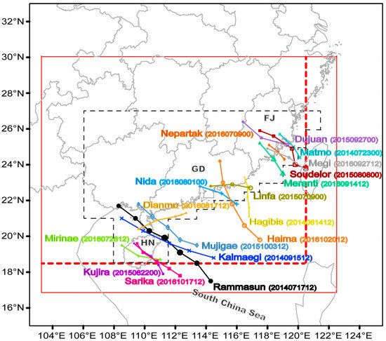
Figure 1.
Tracks of the 17 tropical cyclones (TCs) examined in this study from the CMA best-track analysis. Here, the TC position at the first forecast initialization time is used as the beginning of the track. The sizes of the TC symbols represent the TC intensities, with larger sizes corresponding to stronger TCs; the number in parentheses is the first forecast initialization time (UTC) for the TC; the thin red solid rectangle indicates the domain for GRAPES-MARS3KM, with the thick red dashed lines outlining the “inner range” of GRAPES-MARS3KM; the dashed black rectangle indicates the verification area. ‘FJ’, ‘GD’, and ‘HN’ indicate the ‘Fujian’, ‘Guangdong’, and ‘Hainan’ provinces, respectively.
Both the Lateral Boundary Conditions (LBCs) for GRAPES-MARS3KM and the first background field for DA are determined from DETER. However, due to the limited range of TREPS, both the LBCs and the first background field provided by the DETER cannot adequately cover the domain of GRAPES-MARS3KM for some TC cases. In such cases, the HRES forecasts are used.
2.2. Partial-Cycle DA System
The DA system used here is GRAPES-CHAF3KM [Z16], which is based on the GRAPES 3D-Var framework [35,46] along with the multigrid technique [47] and the partial cycling strategy [48].
The GRAPES 3D-Var framework uses the incremental 3D-Var analysis scheme [49], which is similar to that used with the Weather Research and Forecasting model [50]. The cost function is as follows:
where and denote the analysis and background fields, respectively, and denotes the observation vector; denotes the observation operator; the background and observation error covariance matrices are denoted by and , respectively. Stream function, velocity potential, unbalanced Exner pressure, and pseudo–relative humidity are used as control variables in this system. In GRAPES 3D-Var, a linear balance equation which contains the curvature function is used to improve the balance between the wind and pressure in TCs. The background error covariances are estimated by the innovation vector method [51] and then tuned to meet the needs of assimilation for the convection-permitting model.
Recently, the multi-grid technique was proposed to assimilate the multi-scale information of observations on grids with different resolutions [47]. The cost function used in the multi-grid technique is as follows:
where n denotes the grid level with the total grid levels equaling N. The final analysis is the sum of the incremental analyses at all grid levels:
where denotes the solution of the minimization at the nth grid level. In the current GRAPES 3D-Var, only two grid levels (i.e., N = 2) are used. Based on the multigrid technique, a two-step 3D-Var analysis is conducted. First, the large-scale background fields are generated by projecting the model grid onto a coarse grid containing half the number of domain grid points, then the corresponding large-scale analyses are produced by 3D-Var analysis with the large-scale background error covariances with larger-scale length scales. Second, the large-scale analyses are interpolated onto the model grid to create the new small-scale background fields, then the corresponding small-scale analyses are produced via 3D-Var analysis with the small-scale background error covariances with smaller-scale length scales and adopted as the final analyses. Currently, this multi-grid GRAPES 3D-Var scheme has been applied in both the heavy rainfall [39] and TC [52] forecasting in Southern China. The 6-h partial cycling strategy is implemented as follows. A cold start of multi-grid 3D-Var analysis is activated 6 h prior to the initial time of the 12-h forecasts, with the forecasts of DETER or ECMWF HRES as the background fields. Subsequent assimilation cycles are run at an interval of 3 h, with the 3-h forecasts of GRAPES-MARS3KM issued from the previous analysis as the background fields.
2.3. Experimental Design
Analysis-forecast cycles based on GRAPES-CHAF3KM and GRAPES-MARS3KM were carried out, with the focus on the TCs making landfall on Southern China during 2014–2016. The configuration of these analysis-forecast cycles is shown in Figure 2. According to the TC track forecasting from TREPS EM, if the target TC is predicted to land in 24–36 h, the 6-h DA cycling with GRAPES-CHAF3KM and the subsequent 12-h forecasts with GRAPES-MARS3KM initiate per 12 h unless the target TC has made landfall before the initial time. Note that, if the target TC is predicted by TREPS EM to be located outside the “inner range” of GRAPES-MARS3KM (Figure 1) at the time when the cold start of GRAPES-CHAF3KM initiates, the corresponding analysis-forecast cycles are not conducted, because the TC circulation is not well covered by the domain of GRAPES-MARS3KM. Here, if the range from the target TC center to the half of the surface-wind radius of 17.2 m s−1 (gale_radius, hereafter), which is reported in WARNING, is completely outside the inner range of GRAPES-MARS3KM, the TC is defined outside the inner range. During the experimental period, 17 TC cases (Figure 1) with 28 12-h forecasts were collected.
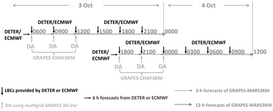
Figure 2.
Schematic configuration of the analysis-forecasts cycles using GRAPES-CHAF3KM and GRAPES-MARS3KM. The analysis-forecasts cycles for TC Mujigae are shown as an example. ECMWF: European Centre for Medium-range Forecasts (HRES); DETER: control (deterministic or unperturbed) forecasts of TREPS; GRAPES: Global/Regional Assimilation and Prediction System.
Two experiments, namely control (CTL) and assimilation of OPT-derived observations (AOPT) respectively, were conducted to investigate the impacts of assimilating OPT-derived observations on TC forecasting of GRAPES-MARS3KM. Data from four types of observation (see Figure 1a of [Z16] for the distributions), i.e., radiosonde, surface station, ship, and wind-profiling radar, were assimilated in CTL. AOPT was identical to CTL except that OPT-derived observations were also assimilated. The impact of assimilating OPT-derived observations was thus evaluated by comparing the skill scores, which are introduced below, between CTL and AOPT.
2.4. Forecast Verification
Similar to [Z18], the TC center in this study is defined as the minimum of the geopotential height at 850 hPa (For all the TC cases examined in this study, the comparison between the TC center based on the minimum of the 850-hPa geopotential height and the center of the 850-hPa TC circulation showed small departures between each other), while the lowest SLP within 100 km of the TC center is used to define the minimum central pressure, viz. Pmin, and the highest 10-m wind speed within 250 km of the TC center is used to define the maximum sustained wind speed, viz. Vmax. The CMA best-track dataset ([53]; http://tcdata.typhoon.gov.cn) was used to calculate the absolute track, Pmin and Vmax error over the set of 28 forecasts. To ensure a fair comparison, a homogeneous sample of TC cases with observed or predicted Vmax larger than 10 m s−1 was used.
Forecasts of 1-h accumulated rainfall and 10-m wind were verified against hourly rainfall and 10-m wind observations respectively, from the automatic weather stations (AWSs) densely distributed over Southern China (see Figure 1b of [Z16] for the distributions). Both rainfall and 10-m wind observations were interpolated to the NWP model grids with Cressman interpolation to calculate skill scores. Fraction skill score (FSS; [54]) was computed for the 1-h accumulated rainfall and 10-m wind in consideration of the more significant “double penalties” due to the displacement error in the verification of high-resolution forecasts [55]. In calculating FSS, “neighborhood length” was defined as the length of area over which the fractions were computed. FSS was calculated for varying precipitation thresholds over different neighborhood lengths. However, only the 50-km-length FSS was compared between various forecasts here, as in [56], because the conclusions based on the comparison of FSS with other neighborhood lengths are nearly the same. FSS ranges from 0 to 1, with higher values corresponding to higher skills.
The skill scores, i.e., absolute track/intensity error and FSS, were computed by averaging over the 28 forecasts and the verification area (Figure 1). For the comparison of these skill scores, statistical significances of the differences between different forecasts, e.g., CTL and AOPT, were assessed using a bootstrap resampling procedure. Specifically, random samples of skill scores were generated with replacement, and then the differences of skill scores were calculated. This procedure was repeated 1000 times and bootstrapping was performed on the score differences between the paired samples. The rank at which the resampled score differences crossed zero was used as the significance level [11] to represent the probability that two skill scores were distinct. Here, a 90% significance level indicates a 90% probability that two skill scores differ.
2.5. Cases Overview
Most of the 17 TCs moved northwestward from the Western North Pacific or SCS to the southeast coast of China and mainly made landfall on the Fujian (FJ), Guangdong (GD), and Hainan (HN) provinces. For TCs evolved around the northeast of the model domain, the description of steering flows from the subtropical ridge in GRAPES-MARS3KM is generally insufficient, because the subtropical ridge only covers the limited area of the model domain. In order to quantitatively identify such TCs, the distances between the observed TC center, which is reported in WARNING, and the northern and eastern lateral boundaries are respectively calculated and averaged over all the analysis times. For a given TC case, if the sum of these two distances is smaller than 10.5°, it is classified as “northeast TC”. Among the 17 TCs, northeast TCs include Matmo, Soudelor, Dujuan, Meranti, and Megi. For such TC cases, the forecast performances of track based on OPT are overall poorer than those for the other TC cases (not shown), which are classified as “non-northeast TCs”.
Mujigae, the strongest TC making landfall on GD in October since 1949, landed on GD at around 0600 UTC 4 Oct 2015 with Pmin of 935 hPa and Vmax of 52 m s−1. Accompanied by several TC-spawned tornadoes, Mujigae had caused great damage in GD [57,58]. Mujigae entered SCS at 0200 UTC 2 October and strengthened rapidly with Vmax increasing from 28 (at 0600 UTC 3 Oct) to 50 (at 0600 UTC 4 Oct) m s−1. In view of the serious nature of the resulting disaster and its rapid intensification (RI), which is difficult to be skillfully predicted currently [17], Mujigae was selected as the case study.
3. OPT-Derived Data and Preprocessing
3.1. Construction of OPT
TREPS comprises one unperturbed and 30 perturbed forecasts ranging up to 60 h at 0.09° horizontal resolution. The 30 60-h perturbed forecasts are used to construct OPT, which provide 60-h deterministic forecasts. Specifically, a single member was selected to be OPT based on the closeness of the perturbed ensemble members’ forecasts to both EM forecasts (for both track and intensity) and the latest observations of WARNING. OPT was determined by minimizing a cost function as follows:
The first term on the right-hand side of Equation (4) measures the closeness to the latest observations, where , , and denote absolute errors of the track, Pmin, and Vmax, respectively, against WARNING observations for member at lead time ; is the weighting factor depending on the Pmin observation at lead time . The second term on the right-hand side measures the closeness to EM forecasts, where , , and denote absolute differences of the track, Pmin, and Vmax, respectively, compared with EM forecasts for member at lead time . , , and denote the standard deviation of the TC track (15 km), Pmin (4 hPa), and Vmax (1 m s−1), respectively, which are used to normalize the various variables to maintain their mutual balance. If more than one member had a minimum cost function, OPT were produced by averaging over these members.
3.2. Data Derived from OPT
For each grid point in OPT, if its distance from the observed TC center reported in WARNING was smaller than the gale_radius, the corresponding variables located at this grid point were selected to be derived. Considering that OPT is a type of forecast product, the variables derived from OPT are probably characterized by spatial correlations in the forecast error. Thus, when OPT-derived data were used as the pseudo observations, these observations may be horizontally correlated, implying that there are probably correlations in the “observation error”. In order to reduce the impacts of correlated observation errors on DA, data thinning has been widely used [59,60,61]. Consequently, the grid points of OPT were selected at an interval of 5. Because the horizontal resolution of TREPS is 0.09° × 0.09°, the horizontal resolution of OPT-derived data is about 45 km (Figure 3a).
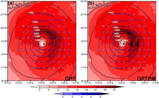
Figure 3.
Horizontal distributions of 850-hPa geopotential height (contours with interval of 20 gpm) and 10-m wind speed (shaded, unit: m s−1) at 0600 UTC 3 Oct 2015 from OPT (a) and OPTPM (b). The dots indicate the grid points used to construct the OPT- and OPTPM-derived data, with different colors representing different ensemble spreads of 10-m wind speed (unit: m s−1), which are calculated as the square root of the sum of the squared 10-m-U and 10-m-V ensemble spreads. The green plus indicates the location of the TC center reported in WARNING.
U, V, geopotential height, temperature (T), and relative humidity (RH), which were derived from OPT at 1000, 925, 850, 700, 600, 500, 400, 300, 250, 200, 150, and 100 hPa, were used in a similar way to radiosonde observations. The surface variables from OPT, including SLP, 10-m U, 10-m V, 2-m T, and 2-m RH, were used to construct the OPT-derived data in a similar way to surface observations.
3.3. Data Derived from OPTPM
As illustrated in [Z18], when OPT was used, there were some mixed results with some degradations in strong and extremely strong wind in TREPS forecasts. These degradations were caused by the excessive smoothing in OPT fields, due to simple averaging over the ensemble members with nearly the same minimum cost function, which was used to determine the optimal members. Thus, underestimations were probably present in the OPT-derived data, especially for strong wind. For Mujigae, the observed Vmax at 0600 UTC 3 Oct 2015 was 33 m s−1. However, in OPT fields, which were produced by averaging two ensemble members, the area around predicted TC center with Vmax exceeding 27 m s−1 was very limited (Figure 3a), indicating insufficient ability of OPT to describe strong TCs.
In order to cope with the issue of simply averaging all ensemble members, PM was proposed by [62] by blending the spatial pattern of EM fields with the frequency distribution of the whole EPS. Thus, it seems that the PM technique could be used to partially address the underestimations in OPT. In this study, a new TREPS product based on both the OPT and PM techniques, namely OPTPM, was constructed in three steps. First, the frequency distribution was formed by pooling predicted fields (e.g., 10-m U) from N ensemble members of TREPS, which were all selected to construct OPT, at each grid point in the domain of the OPT-derived data, ranking them from largest to smallest and keeping every Nth value. Second, OPT fields in the domain of the OPT-derived data were also ranked from largest to smallest. Third, the grid point corresponding to the largest OPT fields was assigned the largest value in the frequency distribution, and so on. An example of the OPTPM-derived data is shown in Figure 3b. Compared with OPT fields (Figure 3a), OPTPM fields described a stronger TC with higher 10-m wind speed and lower SLP (Figure 3b). The differences in magnitude between OPT and OPTPM fields were more evident around the predicted TC center, where the excessive smoothing in OPT fields was more serious. Note that, because the patterns of OPT fields were the same as those of OPTPM fields, the locations of the TC center and thus the TC tracks did not differ between OPT and OPTPM.
The third experiment, namely AOPM, was thus conducted to investigate the impacts of assimilating OPTPM-derived observations on TC forecasting. AOPM was identical to AOPT except that the OPTPM-derived data instead of the OPT-derived data were assimilated.
3.4. Data Accuracy
In order to examine the accuracy of the derived data, the forecast errors of track and Vmax for both the OPT- and OPTPM-derived data were calculated (Figure 4).
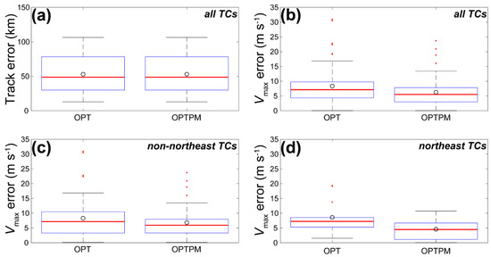
Figure 4.
Box-and-whisker plots for absolute errors of the TC track (a) and Vmax (b–d) with best-track data as the truth over all optimal-member forecast (OPT)- and its probability-matched mean (OPTPM)-derived data used in the analysis for forecasts of all TCs (a,b), non-northeast TCs (c), and northeast TCs (d). The red thick line in the box indicates the median value, the circle represents the mean value, the box shows the interquartile range (i.e., the 25th and 75th percentiles), the horizontal line outside the box (i.e., whiskers) marks the percentiles of 1.5 times the interquartile range, and points outside the whisker are outliers.
As illustrated above, the tracks were the same between OPT- and OPTPM-derived data, thus, the absolute track errors were the same between these two data (Figure 4a). Overall, the absolute track errors of the derived data were smaller than 100 km, with mean track errors around 50 km.
With a few exceptions, the absolute errors of Vmax for the OPT-derived data were generally below 20 m s−1 (Figure 4b). Actually, the larger Vmax errors, e.g., 30 m s−1, were attributed to the stronger TCs, e.g., Rammasun, whose peak maximum Vmax reached 72 m s−1 (Figure 12c of [Z18]). For the OPTPM-derived data, the absolute errors of Vmax were generally below 15 m s−1 (Figure 4b). Thus, compared with the OPT-derived data, the OPTPM-derived data showed some improvements in estimating the TC intensity, with the mean Vmax errors reduced from 8 m s−1 to 6 m s−1. Moreover, the improvements in estimating the TC intensity of the OPTPM-derived data over the OPT-derived data were more evident for northeast TCs (Figure 4d) than for non-northeast TCs (Figure 4c).
Compared with the track (Vmax) uncertainties of some TC best-track data [63], the track (Vmax) errors of the derived data were generally similar although a bit larger, especially for the OPTPM-derived data. Thus, the accuracy of the derived data should be generally acceptable, at least in terms of the TC track and intensity.
3.5. Observation Errors
Both OPT and OPTPM fields are the deterministic products of TREPS, which aim to estimate the true atmospheric state. Thus, the observation errors of the OPT- and OPTPM-derived data are closely related to the forecast uncertainties or errors of OPT and OPTPM fields. It is well known that the ensemble spread provided by EPSs can be used to estimate the forecast uncertainty or error [64]. Therefore, the ensemble spreads from TREPS for various variables, which have been used in the OPT- and OPTPM-derived data, were used to simply estimate their standard deviations of observation errors.
As an example, Figure 3 shows the horizontal distribution of the ensemble spreads from TREPS for 10-m wind speed. These ensemble spreads increased evidently when approaching the predicted TC center of OPT- or OPTPM-derived data, illustrating larger forecast errors around the predicted TC center. This result is not surprising, because divergence of predicted TC locations between ensemble members often leads to the most evident divergence of predicted surface wind occurring around the ensemble-mean TC center. Additionally, the regions with strong surface wind especially in the northeast quadrant, which are often characterized by large forecast errors (e.g., [19,65]), corresponded well with those with large ensemble spreads (Figure 3). This indicated that the ensemble spread provided by TREPS can estimate the observation error of the derived data to some extent.
However, as shown in Figure 3, the ensemble spread generally ranged from 2 to 6 m s−1, which was evidently larger than the standard deviation of observation errors for some conventional observations, e.g., radiosonde [66]. Consequently, the analysis increments due to assimilating the derived data would be evidently smaller than those due to assimilating conventional observations, if the ensemble spread was directly used as the estimation of observation errors. To increase the impacts of assimilating the derived data on the analyses, 50% of the ensemble spread was used as the standard deviation of observation errors for both the OPT- and OPTPM-derived data. Actually, some sensitivity experiments, in which the ensemble spread was scaled as 25%, 50%, 75%, and 100% of the original estimate, were conducted for two typical TC cases, which were Mujigae and Soudelor. Among these sensitivity experiments, those with 50% of the ensemble spread as the standard deviation of observation errors showed the best performance in both the TC track and TC intensity forecasting. Especially, 40% of the ensemble spread was used for the OPTPM-derived data in the northeast TC cases, considering the obvious improvements of OPTPM over OPT in estimating the TC intensity for northeast TCs (Figure 4d). Note that, observation errors of the OPT- and OPTPM-derived data were probably underestimated here. In order to avoid the excessive impacts of the derived data (especially those with poor qualities) on DA, the derived data must be further quality controlled (see the below section).
3.6. Quality Control
The quality control (QC) is essential for the derived data, given that such data are in fact based on forecasts of NWP models and are thus characterized by inevitable forecast errors. QC applied here followed two steps.
Firstly, with the TC track and Vmax reported in WARNING as the truth, the Vmax bias, track error, and Vmax error of TC in OPT fields were calculated and averaged over all the analysis times during the 6-h DA cycle. If one of the three situations occurred, that is, the Vmax bias, track error, and Vmax error were larger than 5 m s−1, 100 km, and 20 m s−1, respectively, both the OPT- and OPTPM-derived data were treated as erroneous data and thus not used in DA. In this case, both AOPT and AOPM were the same as CTL. Actually, the 28 forecasts corresponding to the 17 TC cases (Figure 1) were determined after implementing such QC. Note that, the derived data with large overestimations of TC Vmax were excluded, because assimilation of such data tended to aggravate the intensity overestimation for weaker TCs in GRAPES-MARS3KM (not shown). After removing the above data, the distributions of the TC Vmax bias, track error, and Vmax error for the OPT-derived data used in this study are shown in Figure 5b–d.
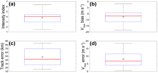
Figure 5.
Box-and-whisker plots for the intensity index (a), which was calculated as the ratio of Vmax to Pmin, and then inflated 100 times and averaged over all the analysis times (unit: m s−1 hPa−1), and the Vmax bias (b), track error (c), and Vmax error (d) with official real-time warning information from CMA (WARNING) as the truth over all OPT-derived data used in the analysis for all the 28 forecasts. The red thick line in the box indicates the median value, the circle represents the mean value, the box shows the interquartile range (i.e., the 25th and 75th percentiles), the horizontal line outside the box (i.e., whiskers) marks the percentiles of 1.5 times the interquartile range, and points outside the whisker are outliers.
Secondly, observations of the derived data were further quality controlled by comparing the innovations, which were the differences between observations and background fields, with the standard deviation of observation errors. In GRAPES 3D-Var, if the innovations exceed qc times the standard deviation, the observations are assumed to be erroneous and thus not assimilated. Therefore, the value of qc determined how many observations can be assimilated. Considering that there were different characteristics in terms of forecast errors between different TCs for both OPT and OPTPM fields (Figure 4), different values of qc were set for different TCs as follows.
(1) Since TCs with different intensities show different characteristics of forecast or estimation errors [13,63], intensity index was defined here to divide all the 17 TCs into three groups. Specifically, intensity index was calculated as the ratio of Vmax to Pmin, which were both reported in WARNING, and then inflated 100 times and averaged over all analysis times. As shown in Figure 5a, intensity index for TCs investigated here ranged from 1 to 7 m s−1 hPa−1, with mean of roughly 4 m s−1 hPa−1. The TC cases with intensity index below 4 m s−1 hPa−1 were defined as “weak TCs”, those above 5 m s−1 hPa−1 were defined as “strong TCs”, while those ranging from 4 to 5 m s−1 hPa−1 were defined as “moderate TCs”. As illustrated in some literatures (e.g., [67,68,69]), lower horizontal resolutions of NWP models probably cannot well represent the intensity of stronger TCs. So, when the derived data, which were based on OPT and OPTPM fields with resolution of roughly 9 km, were used in the DA system with resolution of roughly 3 km, the representative error of the derived data should be larger for stronger TCs. For this reason, values of qc, namely qc1, were set to 5.0, 4.0, and 3.0 for weak, moderate, and strong TCs, respectively.
(2) The track error of OPT fields ranged from 10 to 90 km, with the mean around 50 km (Figure 5c). So, if such track error exceeded 50 km, the corresponding derived data was considered to be characterized by evident track errors. In this case, the value of qc, namely qc2, were set to qc1 − 1 to exclude observations with large innovations in a more rigorous way.
(3) For OPT fields, the ratio of the track error to the gale_radius, which was reported in WARNING, was also calculated and averaged over all the analysis times. If such ratio was larger, the risk that the TC circulation of OPT fields obviously deviated from the observed TC circulation was also larger. Thus, if such ratio exceeded 0.6, the corresponding derived data was thought to probably have detrimental impacts on DA and the value of qc, namely qc3, were set to qc2 − 1.
(4) As illustrated in Section 2.5, OPT fields on average showed better performance in describing the TC track for non-northeast TCs than for northeast TCs. Thus, the value of qc, namely qc4, were set to qc3 − 1 for northeast TCs.
After the above four-step QC, the value of qc can be finally determined. Additionally, the minimum value of qc was restricted to be 1.0. Note that, the above QC used the TC-dependent although somewhat ad hoc qc rather than the fixed or static qc, which is commonly used for real observations. Actually, some sensitivity experiments were carried out for two TC cases, i.e., Mujigae and Kujira, which were representative of TCs with different intensities. These sensitivity experiments showed the superiority of the TC-dependent qc over the fixed qc in TC forecasting (not shown).
4. Results of the Batch Experiment
4.1. Forecasts of TC Track and Intensity
For all the 28 forecasts, there were no statistically significant differences in TC track errors between AOPT or AOPM and CTL at 6-h and 12-h lead times (Figure 6a). However, in terms of the analyzed location of TC center, errors in both AOPT and AOPM were significantly larger than in CTL (Figure 6a). This degeneration of describing initial TC locations of both AOPT and AOPM relative to CTL limited the improvements by assimilating the derived data in the TC track forecasting. Compared with AOPT, AOPM showed some slight improvements in the TC track forecasting, with significant improvements at the 12-h lead times.
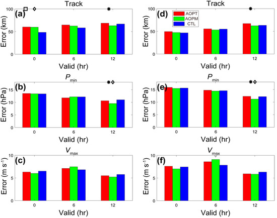
Figure 6.
Absolute errors of the TC track (a,d), Pmin (b,e), and Vmax (c,f) at different lead times, for all the 28 forecasts (a–c) and for the 17 forecasts with the “small-error” derived data assimilated (d–f). Black (gray) squares, diamonds and asterisks indicate the lead times for which the significance level of the absolute error differences is larger than 90% (85%) for the comparisons between assimilation of OPT-derived observations (AOPT) and control (CTL), between assimilation of OPTPM-derived observations (AOPM) and CTL, and between AOPT and AOPM, respectively. The legend in (d) identifies the three experiments shown in these panels.
On average, both AOPT and AOPM showed slightly smaller errors in analyzing and predicting the TC intensity (i.e., Pmin and Vmax) than CTL, especially for Pmin in the later period of the 12-h forecasts (Figure 6b). The degeneration of TC Vmax forecasting of both AOPT and AOPM over CTL at the 6-h lead times is likely the result of the poor spinup process due to assimilating the derived data. The TC intensity errors, with respect to both Pmin and Vmax, were generally similar between AOPT and AOPM, with smaller errors at the 12-h lead times in the latter than in the former (Figure 6b,c).
In summary, assimilating the derived data led to some degenerations (improvements) in analyzing and predicting the TC track (intensity). Recall from Figure 5c,d that there were a few evident deviations of the derived data from WARNING in terms of both track and intensity, with track (Vmax) errors exceeding 50 km (5 m s−1). Obviously, such derived data were characterized by larger errors or worse qualities relative to WARNING than other derived data. The differences in quality between different derived data would potentially lead to differences in the contributions to forecast performance. Did the forecasts with these “large-error” derived data assimilated contribute to the degenerations due to assimilation of the derived data in the analysis and forecast of TC track? It is important to answer this question for further revealing the deficiency of the proposed derived-data assimilation technique. For this purpose, the TC track and intensity errors were recalculated based on the 17 forecasts with the “small-error” derived data assimilated (Figure 6d–f). Here, for both the OPT- and OPTPM-derived data, if their track errors (Figure 5c) were below 50 km or Vmax errors (Figure 5d) were below 5 m s−1, the corresponding data were defined as “small-error” derived data; otherwise, “large-error” derived data were used to identify the corresponding data. The criterions (i.e., 50-km track errors and 5-ms−1 Vmax errors), used to separate the derived data between the “large-error” and the “small-error” ones, were nearly the mean or median values of errors for all TC cases (Figure 5c,d). Besides, there were 17 (11) forecasts with the “small-error” (“large-error”) derived data assimilated, suggesting that the samples were generally comparable between forecasts with “small-error” derived data assimilated and those without. Thus, the comparison between forecasts with derived data of different qualities assimilated should be generally fair.
As shown in Figure 6d, the TC track errors in both AOPT and AOPM became close to those in CTL, after removing the forecasts with the “large-error” derived data assimilated. In this case, assimilating the derived data did not significantly influence the analysis and forecast of TC track. However, for the analysis and forecast of TC intensity, removing the forecasts with the “large-error” derived data assimilated did not further increase but even reduce the advantage of AOPT or AOPM over CTL (Figure 6e,f). The error of initial TC location in CTL was below 50 km over all the 28 forecasts (Figure 6a). Therefore, including the information of some “large-error” derived data would probably degrade the analysis and thus the forecast performance of TC track. However, the case was different for TC intensity. Because the error of initial TC Vmax in CTL was evidently larger than 5 m s−1, additionally assimilating some “large-error” derived data could still improve the analysis and thus the forecast performance of TC intensity.
4.2. Forecasts of Precipitation
Similar to [56], rainfall with precipitation rates greater than 0.1, 10, 20, and 40 mm h−1 is defined as light, moderate, heavy, and extremely heavy rainfall, respectively, in this study.
Compared with CTL, both AOPT and AOPM significantly improved the forecasts of light rainfall during the whole 12-h forecasts (Figure 7a). Moreover, AOPM outperformed AOPT in predicting light rainfall, although the differences were not statistically significant (Figure 7a). However, the advantages of AOPT or AOPM over CTL in predicting light rainfall were not significant for the forecasts with “small-error” derived data assimilated (Figure 7b), which implies that assimilation of “large-error” derived data still benefits the forecasts of rainfall with smaller threshold. As illustrated previously (Figure 6), assimilation of “large-error” derived data led to some improvements (degenerations) in predicting the TC intensity (track). Probably, such degenerations in predicting the TC location do not necessarily cause degenerations in predicting the whole TC circulation, which is closely related to the distribution of light rainfall, because the differences of TC track errors between all the 28 forecasts and the forecasts with “small-error” derived data assimilated were below 15 km (comparing Figure 6a,d), which are evidently smaller than the size of TC circulation. On the contrary, improvements in predicting the TC intensity due to assimilation of “large-error” derived data can improve the forecasts of TC circulation and thus light rainfall, especially for AOPM (comparing Figure 7a,b).
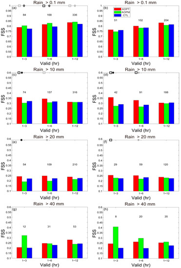
Figure 7.
Fraction skill score (FSS) for forecasts of 1-h accumulated precipitation with thresholds of 0.1 (a,b), 10 (c,d), 20 (e,f), and 40 (g,h) mm and a neighborhood length of 50 km averaged over lead times from 1 to 3 h, 1 to 6 h, and 1 to 12 h, respectively, for all the 28 forecasts (left column) and for the 17 forecasts with the “small-error” derived data assimilated. Black numbers in the top of bars represent the numbers of FSS samples used to calculate the averaged FSS during different lead times. Black (gray) squares, diamonds and asterisks indicate the lead times for which the significance level of the absolute error differences is larger than 90% (85%) for the comparisons between AOPT and CTL, between AOPM and CTL, and between AOPT and AOPM, respectively. The legend in (e) identifies the three experiments shown in these panels.
For the forecasts of moderate rainfall, AOPT showed significantly improvements over both AOPM and CTL in the first few hours (Figure 7c). However, for the performance during the whole 12-h forecasts, assimilating the OPT- or OPTPM-derived data did not bring significant improvements (Figure 7c). These conclusions are valid for all the forecasts, regardless of whether “large-error” or “small-error” derived data were assimilated (Figure 7c,d). Considering that the distribution of moderate rainfall should be closer to the TC center than that of light rainfall, degenerations caused by assimilating “large-error” derived data in the TC location forecasting are likely more evident for predicting moderate rainfall than light rainfall. Consequently, such degenerations in predicting the TC location might compensate for the improvements in predicting the TC intensity and thus result in marginal impacts of excluding “large-error” derived data on DA.
Comparison between AOPT and CTL showed that, assimilation of the OPT-derived data resulted in consistent improvements in predicting heavy rainfall during the whole 12-h forecasts (Figure 7e). Assimilating the OPTPM-derived data seemed to degrade the forecasts of heavy rainfall, although the degradations were not statistically significant (Figure 7e). If only “small-error” OPT- or OPTPM-derived data were assimilated, the forecasts of heavy rainfall can be slightly improved, especially for the former (latter) during the first (last) few hours (Figure 7f). Obviously, improvements in predicting the TC intensity due to assimilating “large-error” derived data were overwhelmed by degenerations in predicting the TC location, which were highly related to the forecasts of heavy rainfall.
Due to limited observations or forecast samples for extremely heavy rainfall, the forecast differences among CTL, AOPT, and AOPM were not statistically significant; although the positive impacts of assimilating the derived data were still observed in some lead times (Figure 7g). Similar to heavy rainfall, excluding “large-error” derived data in DA increased the positive impacts of the derived data assimilation on the forecasts of extremely heavy rainfall, especially for AOPM (Figure 7h).
In summary, assimilation of the OPT-derived data was beneficial to the TC precipitation forecasting at some thresholds, with significant impacts on lighter rainfall. Significant positive impacts of assimilating the OPTPM-derived data were limited to the forecasts of light rainfall. The forecast differences of precipitation between AOPT and AOPM, especially for moderate and heavy rainfall, are attributed to the forecast differences of TC intensity, because both of the predicted precipitation (Figure 7a,c,e) and TC intensity (Figure 6b,c) were better (worse) during the last (first) few hours in AOPM than in AOPT. To improve the forecasts of heavier rainfall, it is better to assimilate “small-error” instead of “large-error” derived data, especially for the OPTPM-derived data.
In order to further investigate the impact of assimilating “small-error” derived data on heavy rainfall, the 25-km FSS was also compared between different experiments (Figure 8a). The improvements in predicting heavy rainfall of AOPM over AOPT and CTL progressed when the neighborhood length of FSS decreased, illustrating that the advantage of AOPM over AOPT and CTL was more evident for heavy rainfall with more local scales.

Figure 8.
FSS for forecasts of 1-h accumulated precipitation larger than 20 mm (a) and 10-m wind speed larger than 24.5 m s−1 (b), with neighborhood lengths of 50 (open bars with gray thick borders) and 25 (full bars with black thin borders) km averaged over lead times from 1 to 3 h, 1 to 6 h, and 1 to 12 h, respectively, for the 17 forecasts with the “small-error” derived data assimilated. Percentages in the top of bars represent the relative improvements in FSS of AOPT over CTL (red), AOPM over CTL (green), and AOPM over AOPT (black) during different lead times. The bold (italic) percentages corresponds to the comparison of FSS with neighborhood length of 25 (50) km. The legend in (a) identifies the three experiments shown in these panels.
4.3. Forecasts of Surface Wind
In this study, 10-m wind speed greater than 8.0, 17.2, 24.5, and 32.7 m s−1 is defined as weak, moderate, strong, and extremely strong wind, respectively.
During the whole 12-h forecasts, both AOPT and AOPM significantly underperformed CTL for predicting weak wind (Figure 9a). This result held even if only “small-error” derived data were assimilated (Figure 9b). However, the positive impacts of assimilating the OPTPM-derived data increased when only “small-error” derived data were assimilated, especially in the first few hours (Figure 9b). Furthermore, AOPM showed evident improvements over AOPT in predicting weak wind, especially in the forecasts with “small-error” derived data assimilated.
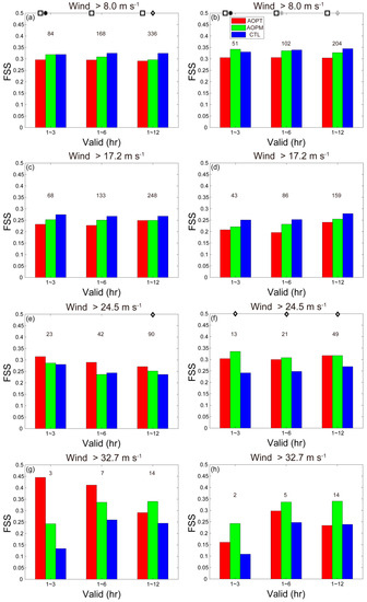
Figure 9.
As in Figure 7, but for 10-m wind speed with thresholds of 8.0 (a,b), 17.2 (c,d), 24.5 (e,f), and 32.7 (g,h) m s−1.
The conclusion for the comparison among AOPT, AOPM, and CTL in the forecasts of moderate wind was roughly similar to that for the forecasts of weak wind, except that the forecast differences among the three experiments were statistically insignificant (Figure 9c,d).
For the forecasts of strong wind during the whole 12-h forecasts, both AOPT and AOPM outperformed CTL, with significant improvements of AOPM over CTL during the last few hours (Figure 9e). Although AOPT showed better performance in predicting strong wind than AOPM, the differences between them were not statistically significant. The positive impacts of assimilating the derived data, especially the OPTPM-derived data, were more evident in the forecasts with “small-error” derived data assimilated than those with “large-error” one assimilated (Figure 9f).
There were no statistically significant differences among CTL, AOPT, and AOPM, because of limited observations or forecast samples for extremely strong wind (Figure 9g). Thus, the positive impacts of assimilating the derived data on the forecasts of extremely strong wind (Figure 9g) were the results based on some strong TC cases (e.g., Rammasun). Moreover, assimilation of the “small-error” OPTPM-derived data showed more positive impacts than that of the “large-error” one (Figure 9h).
In short, the forecast improvements due to assimilating the derived data were mainly limited to strong wind, especially with significant improvements based on the assimilation of the OPTPM-derived data. Again, similar to precipitation, the forecast differences of surface wind between AOPT and AOPM, especially for strong and extremely strong wind (Figure 9e,g), were closely related to the forecast differences of TC intensity (Figure 6b,c). Besides, the positive impacts of assimilating the “small-error” OPTPM-derived data increased with the predicted intensity of surface wind, which was also found in precipitation forecasting and probably attributed to similar reasons.
The positive impacts of assimilating the derived data (especially the OPT-derived data) on the forecasts of strong wind seemed to be weaker in the case of FSS with smaller neighborhood lengths (Figure 8b), illustrating the difficulties in further improving the forecasts of strong wind with more local scales by assimilating the derived data. This result is different from that of heavy rainfall, which may be related to different predictabilities between strong wind and heavy rainfall. However, assimilation of the OPTPM-derived data was more effective in predicting strong wind with more local scales than assimilation of the OPT-derived data.
5. Results of the Case Study
In the case study, two 12-h forecasts, which were respectively initialized at 1200 UTC 3 and 0000 UTC 4 Oct 2015 (Figure 2), were discussed. Note that, the derived data assimilated in these two forecasts were characterized by the “small-error” data.
5.1. Analyses
In the analyses at 1200 UTC 3 October, which served as IC of the 12-h forecasts, there were evident differences for the TC intensity among CTL, AOPT, and AOPM, although the TC sizes were generally similar (Figure 10). Specifically, the analyzed TC was strongest in AOPM (Figure 10c), followed by AOPT (Figure 10b). Recall from Figure 3, where OPT and OPTPM fields derived 6 h earlier are shown, that stronger surface wind was present in OPTPM fields than in OPT fields, especially in the northeast quadrant. Additionally, at the analysis time 6 h earlier, the TC intensities in both OPT and OPTPM fields were larger than that in the analyses of CTL (not shown). Thus, compared with both CTL and AOPT, the stronger TC in IC of AOPM was attributed to the OPTPM-derived data assimilated during the 6-h DA cycle. Moreover, the area characterized by strong wind in AOPT and AOPM was evidently larger than that in CTL. Compared with AOPT, in AOPM, the TC shape was rounder and the strong wind was more widespread although with smaller area.
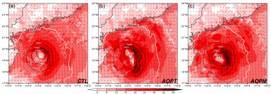
Figure 10.
Analyses for 10-m wind speed (shaded, unit: m s−1) and wind vector (arrows), and geopotential heights at 850 (>1440 gpm; black contours with interval of 40 gpm) and 500 (white contours for values equal to 5880 gpm) hPa at 1200 UTC 3 Oct 2015 from CTL (a), AOPT (b), and AOPM (c).
The initial TC location was also changed, when AOPT or AOPM was compared with CTL. The subtropical ridge, which is indicated by the 5880-gpm contour in Figure 10, located more north in both AOPT and AOPM (Figure 10b,c) than in CTL (Figure 10a). As a result, the TC tracks in both AOPT and AOPM were generally more north than that in CTL during the first 6 h of forecasts (Figure 11).
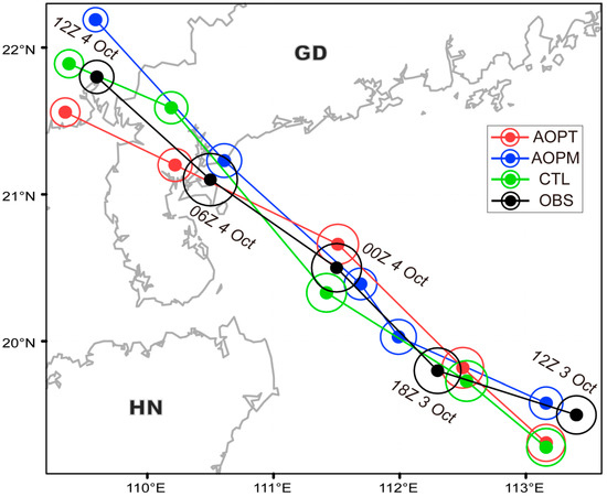
Figure 11.
Observations (black) and forecasts (red, blue, and green) of track (lines), Pmin (dots), and Vmax (circles) for Mujigae from 1200 UTC 3 to 1200 UTC 4 October 2015. The sizes of the dots (circles) represent the TC intensities, with smaller (larger) sizes corresponding to stronger TCs. ‘OBS’ represents the observations from CMA best-track dataset. The start TC location at the lower right corner of the panel indicates the analyses at 1200 UTC 3 October 2015, while the other TC locations indicate the forecasts.
Thus, assimilation of the derived data during the DA cycle can modify not only the TC intensity and structure but also the TC location and steering flow.
5.2. Forecasts
Both AOPT and AOPM did not show consistent advantages over CTL in predicting the TC track, actually with evident advantages mainly in the first 12-h forecasts (Figure 11). Compared with CTL, the underestimation of TC intensity in both AOPT and AOPM was evidently reduced, especially in terms of Vmax (Figure 11). Obviously, these improvements of AOPT or AOPM over CTL in the TC intensity forecasting were closely related to the improved descriptions of TC intensity in the analyses (Figure 10 and Figure 11).
At 1600 UTC 3 October when Mujigae approached HN, moderate wind was observed near the coasts of southwest GD and northeast HN (Figure 12a). Apparently, moderate wind was underestimated in both CTL and AOPT, especially in CTL (Figure 12b,c). Overall, AOPM showed the best performance in predicting moderate wind (Figure 12d), followed by AOPT (Figure 12c). Moreover, strong and even extremely strong wind was observed to occur in the northwest and southwest quadrants of the TC circulation (Figure 12a). Again, AOPM outperformed both AOPT and CTL in predicting the intensity and structure of (extremely) strong wind, although the location error was indeed present (Figure 12d).
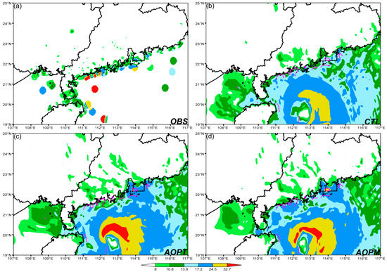
Figure 12.
10-m wind speed (shaded, unit: m s−1) of AWS observation (a) and 4-h forecasts from CTL (b), AOPT (c), and AOPM (d) at 1600 UTC 3 October 2015. The outlines of the observed wind speed are contoured at the 17.2 m s−1 threshold in magenta lines in (b–d).
At 0000 UTC 4 October, i.e., 6 h ahead of the landfall of Mujigae, several rainbands characterized by moderate rainfall occurred in the southwest GD, with heavy and extremely heavy rainfall in some areas (Figure 13a). Among the three experiments, AOPM generally performed best in predicting the observed rainbands in terms of both magnitude and location (Figure 13d). The advantages of AOPT over CTL were limited to predicting the outer rainbands; while for inner rainbands, AOPT behaved worse than CTL (Figure 13b,c).
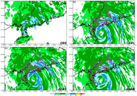
Figure 13.
1-h accumulated rainfall (shaded, unit: mm) of automatic weather station (AWS) observation (a) and 12-h forecasts from CTL (b), AOPT (c), and AOPM (d) at 0000 UTC 4 October 2015. The outlines of the observed rainfall are contoured at the 10 mm threshold in magenta lines in (b–d).
The improvements of AOPM over AOPT and CTL in predicting both the inner and outer rainbands (Figure 13d) were relevant to those in predicting the structure of TC circulation, i.e., wind fields (Figure 12d), because the pattern of TC rainbands was generally similar to that of TC surface wind, especially around the TC inner core. However, the stronger predicted surface wind in AOPM/AOPT than in CTL did not necessarily lead to heavier predicted rainfall. Thus, the underestimation of heavy and extremely heavy rainfall in CTL was not well alleviated in both AOPM and AOPT.
6. Conclusions and Discussion
In order to partially address the difficulty that insufficient inner-core observations have been assimilated in the current convection-permitting NWP model in Southern China, which has severely limited the operational forecast skill of landfalling TCs, assimilation of the pseudo observations derived from some deterministic products of TREPS was implemented in this study.
Both OPT and OPTPM fields from TREPS were used to derive pseudo observations with the horizontal resolution of roughly 45 km. The derived data generally showed acceptable accuracy, compared with the TC track and Vmax uncertainties of some best-track data. And the estimation of TC intensity was more accurate in the OPTPM-derived data than in the OPT-derived data, because the excessive smoothing in OPT fields can be avoided in OPTPM fields. The ensemble spreads from TREPS after some scaling processes were used to simply estimate the standard deviations of observation errors for the derived data. A series of QC steps were carried out to reduce the impacts of inevitable forecast errors present in the derived data on DA.
The impact of assimilating the derived data on the 12-h forecasts of TC track, intensity, precipitation and surface wind was examined by conducting a batch experiment covering 17 TCs making landfall in Southern China during 2014–2016. This batch experiment included 28 analysis-forecast cycles based on the GRAPES-CHAF3KM DA system and GRAPES-MARS3KM model whose horizontal resolution is about 3 km. The control experiment (CTL) without the derived data assimilated was compared with the experiments, namely AOPT and AOPM, with the OPT- and OPTPM-derived data assimilated respectively.
Verification of the TC track forecasting indicated the statistically insignificant impacts of assimilating the derived data, which was due to the degeneration of describing initial TC location caused by the assimilation of derived data. Furthermore, compared with the OPT-derived data, assimilating the OPTPM-derived data slightly improved the TC track forecasting at later lead times. Overall, both the analysis and forecast of TC intensity were slightly improved by assimilating the derived data, especially in the later period of the 12-h forecasts. Similar performances of TC intensity forecasting were found between AOPT and AOPM, although AOPM outperformed AOPT at later lead times. Assimilating the “large-error” derived data, which were characterized by track (Vmax) errors exceeding 50 km (5 m s−1) compared with WARNING, degraded both the analysis and forecast of TC track, but it could still improve the analysis and forecast of TC intensity.
Assimilating the OPT-derived data brought improvements in predicting the TC precipitation at some thresholds, especially the lighter rainfall. Limited benefits of assimilating the OPTPM-derived data were found in the forecasts of light rainfall, besides, the negative impacts, albeit statistically insignificant, on TC Vmax forecasting in the first few hours probably limited the positive impacts on the forecasts of heavier rainfall. Assimilation of the “small-error” derived data, especially the OPTPM-derived data, which were characterized by track errors below 50 km or Vmax errors below 5 m s−1 compared with WARNING, improved the forecasts of heavier rainfall. And this positive impact was more evident for heavy rainfall with more local scales.
The forecasts of strong wind were improved by assimilating the derived data, especially the OPTPM-derived data. Moreover, assimilation of the “small-error” OPTPM-derived data can further improve the forecasts of stronger wind. Although the further improvement in the forecasts of strong wind with more local scales by assimilating the derived data was limited, assimilation of the OPTPM-derived data was more effective to address this difficulty than assimilation of the OPT-derived data.
A case study focused on the TC Mujigae, with the corresponding derived data identified as the “small-error” one, was used to intuitively demonstrate the impacts of assimilating the derived data. For this case, assimilation of the derived data (especially the OPTPM-derived data) during the 6-h DA cycle improved the representation of initial TC circulation by improving the description of TC intensity and structure in the analyses, which thus led to the improvements in the forecasts of TC intensity, surface wind, and precipitation. The initial TC location and steering flow were also modified by assimilating the derived data; however, the TC track forecasting did not be improved consistently.
The above conclusions highlight some values of assimilating the derived data from TREPS in landfalling TC forecasting for some variables, e.g., intensity, heavier rainfall, and stronger wind. However, neutral or negative impacts have been also observed for some variables, e.g., track and weaker wind, which strongly calls for further improvements in the technique of assimilating the derived data. Obviously, the accuracy of derived data highly depends on the forecast performance of deterministic products of EPSs, which definitely benefits from the improvements in EPSs. Thus, developments of EPSs, especially their deterministic guidance, are essential for further improvements in the derived data assimilation. Moreover, there are some ad hoc setups in the preprocessing of derived data, e.g., selecting the grid points, determining the observation errors, and QC, which are of relevance to the information derived from EPSs. Therefore, improvements of these setups in future works will further improve the effectiveness of the derived data assimilation. However, the current ad hoc setups are still excessive and would probably limit the broader applicability of the derived data assimilation. Most of these setups are used to address the deficiency due to the poor quality of the derived data in DA. Hence, improving the quality of the derived data will reduce the requirement of ad hoc setups and thereby widen the applicability of the derived data assimilation. More ground-based observations, especially those located around the coast, such as Doppler radar, should also be assimilated along with the derived data, because both the coverage and accuracy of derived data are still insufficient to fully describe the TC circulation. Consequently, the experiments incorporating the derived data and more observations will be conducted in a future study. Considering less observations and forecast samples (especially for extremely heavy rainfall and extremely strong wind) used in this study, more experiments covering more TC cases are needed to draw general conclusions about the performance of assimilating the derived data in TC forecasting, which is very necessary for prompting the assimilation of EPS-derived data in operation.
Author Contributions
X.Z. developed the methods, designed and performed the experiments, and wrote the manuscript; M.C. provided thorough reviews of the earlier version of the manuscript and revised some of the figures.
Funding
This work was supported by the National Basic Research and Development Project (973 program) of China (2015CB452802), Meteorology Public Welfare Scientific Research Projects (GYHY201506022), National Key R&D Program of China (2017YFC1501603), and Natural Science Foundation of Guangdong Province (2017A030313225, 2016A03031000).
Conflicts of Interest
The authors declare no conflict of interest.
References
- Rappaport, E.N.; Franklin, J.L.; Avila, L.A.; Baig, S.R.; Beven, J.L., II; Blake, E.S.; Burr, C.A.; Jing, J.G.; Juckins, C.A.; Knabb, R.D.; et al. Advances and challenges at the National Hurricane Center. Weather Forecast. 2009, 24, 395–419. [Google Scholar] [CrossRef]
- Goldenberg, S.B.; Gopalakrishnan, S.G.; Tallapragada, V.; Quirino, T.; Marks, F.; Trahan, S.; Zhang, X.; Atlas, R. The 2012 Triply-Nested, High-Resolution Operational Version of the Hurricane Weather Research and Forecasting System (HWRF): Track and Intensity Forecast Verifications. Weather Forecast. 2015, 30, 710–729. [Google Scholar] [CrossRef]
- Gopalakrishnan, S.; Toepfer, F.; Gall, R.; Marks, F.; Rappaport, E.N.; Tallapragada, V.; Forsythe-Newell, S.; Aksoy, A.; Bao, J.W.; Bender, M.; et al. 2015 HFIP R&D Activities Summary: Recent Results and Operational Implementation; HFIP Technical Report: HFIP2016-1; NOAA: Washington, DC, USA, 2016.
- Yu, H.; Chen, P.; Li, Q.; Tang, B. Current Capability of Operational Numerical Models in Predicting Tropical Cyclone Intensity in the Western North Pacific. Weather Forecast. 2013, 28, 353–367. [Google Scholar] [CrossRef]
- DeMaria, M.; Sampson, C.R.; Knaff, J.A.; Musgrave, K.D. Is Tropical Cyclone Intensity Guidance Improving? Bull. Am. Meteorol. Soc. 2014, 95, 387–398. [Google Scholar] [CrossRef]
- Cangialosi, J.P.; Franklin, J.L. National Hurricane Center Forecast Verification Report. 2015 Hurricane Season; Presented at NWS; NOAA: Washington, DC, USA, 2016.
- Nishijima, K.; Maruyama, T.; Graf, M. A preliminary impact assessment of typhoon wind risk of residential buildings in Japan under future climate change. Hydrol. Res. Lett. 2012, 6, 23–28. [Google Scholar] [CrossRef]
- Chen, S.S.; Zhao, W.; Donelan, M.A.; Tolman, H.L. Directional Wind–Wave Coupling in Fully Coupled Atmosphere–Wave–Ocean Models: Results from CBLAST-Hurricane. J. Atmos. Sci. 2013, 70, 3198–3215. [Google Scholar] [CrossRef]
- Shi, X.; Liu, S.; Yang, S.; Liu, Q.; Tan, J.; Guo, Z. Spatial–temporal distribution of storm surge damage in the coastal areas of China. Nat. Hazards 2015, 79, 237–247. [Google Scholar] [CrossRef]
- Wang, Y.; Wen, S.; Li, X.; Thomas, F.; Su, B.; Jiang, T.; Wang, R. Spatiotemporal distributions of influential tropical cyclones and associated economic losses in China in 1984–2015. Nat. Hazards 2016, 84, 2009–2030. [Google Scholar] [CrossRef]
- Davis, C.; Wang, W.; Dudhia, J.; Torn, R. Does Increased Horizontal Resolution Improve Hurricane Wind Forecasts? Weather Forecast. 2010, 25, 1826–1841. [Google Scholar] [CrossRef]
- Gopalakrishnan, S.G.; Goldenberg, S.; Quirino, T.; Zhang, X.; Marks, F.; Yeh, K.-S.; Atlas, R.; Tallapragada, V. Toward Improving High-Resolution Numerical Hurricane Forecasting: Influence of Model Horizontal Grid Resolution, Initialization, and Physics. Weather Forecast. 2012, 27, 647–666. [Google Scholar] [CrossRef]
- Xue, M.; Schleif, J.; Kong, F.; Thomas, K.W.; Wang, Y.; Zhu, K. Track and Intensity Forecasting of Hurricanes: Impact of Convection-Permitting Resolution and Global Ensemble Kalman Filter Analysis on 2010 Atlantic Season Forecasts. Weather Forecast. 2013, 28, 1366–1384. [Google Scholar] [CrossRef]
- Zou, X.; Xiao, Q. Studies on the Initialization and Simulation of a Mature Hurricane Using a Variational Bogus Data Assimilation Scheme. J. Atmos. Sci. 2000, 57, 836–860. [Google Scholar] [CrossRef]
- Torn, R.D.; Hakim, G.J. Ensemble Data Assimilation Applied to RAINEX Observations of Hurricane Katrina (2005). Mon. Weather Rev. 2009, 137, 2817–2829. [Google Scholar] [CrossRef]
- Zhang, F.; Weng, Y.; Gamache, J.F.; Marks, F.D. Performance of convection-permitting hurricane initialization and prediction during 2008-2010 with ensemble data assimilation of inner-core airborne Doppler radar observations. Geophys. Res. Lett. 2011, 38, 15810. [Google Scholar] [CrossRef]
- Rogers, R.; Aberson, S.; Aksoy, A.; Annane, B.; Black, M.; Cione, J.; Dorst, N.; Dunion, J.; Gamache, J.; Goldenberg, S.; et al. NOAA’S Hurricane Intensity Forecasting Experiment: A Progress Report. Bull. Am. Meteorol. Soc. 2013, 94, 859–882. [Google Scholar] [CrossRef]
- Xiao, Q.; Zou, X.; Wang, B. Initialization and Simulation of a Landfalling Hurricane Using a Variational Bogus Data Assimilation Scheme. Mon. Weather Rev. 2000, 128, 2252–2269. [Google Scholar] [CrossRef]
- Weng, Y.; Zhang, F. Assimilating Airborne Doppler Radar Observations with an Ensemble Kalman Filter for Convection-Permitting Hurricane Initialization and Prediction: Katrina (2005). Mon. Weather Rev. 2012, 140, 841–859. [Google Scholar] [CrossRef]
- Lau, W.K.; Susskind, J.; Brin, E.; Riishojgaard, L.P.; Reale, O.; Liu, E.; Fuentes, M.; Rosenberg, R. AIRS impact on the analysis and forecast track of tropical cyclone Nargis in a global data assimilation and forecasting system. Geophys. Res. Lett. 2009, 36. [Google Scholar] [CrossRef]
- Wang, P.; Li, J.; Li, Z.; Lim, A.H.N.; Li, J.; Schmit, T.J.; Goldberg, M.D. The Impact of Cross-track Infrared Sounder (CrIS) Cloud-Cleared Radiances on Hurricane Joaquin (2015) and Matthew (2016) Forecasts. J. Geophys. Res. Atmos. 2017, 122, 13–201. [Google Scholar] [CrossRef]
- Schwartz, C.S.; Liu, Z.; Chen, Y.; Huang, X.-Y. Impact of Assimilating Microwave Radiances with a Limited-Area Ensemble Data Assimilation System on Forecasts of Typhoon Morakot. Weather Forecast. 2012, 27, 424–437. [Google Scholar] [CrossRef]
- Zou, X.; Weng, F.; Zhang, B.; Lin, L.; Qin, Z.; Tallapragada, V. Impacts of assimilation of ATMS data in HWRF on track and intensity forecasts of 2012 four landfall hurricanes. J. Geophys. Res. Atmos. 2013, 118, 11–558. [Google Scholar] [CrossRef]
- Zhang, M.; Zupanski, M.; Kim, M.-J.; Knaff, J.A. Assimilating AMSU-A Radiances in the TC Core Area with NOAA Operational HWRF (2011) and a Hybrid Data Assimilation System: Danielle (2010). Mon. Weather Rev. 2013, 141, 3889–3907. [Google Scholar] [CrossRef]
- Xu, D.; Min, J.; Shen, F.; Ban, J.; Chen, P. Assimilation of MWHS radiance data from the FY-3B satellite with the WRF Hybrid-3DVAR system for the forecasting of binary typhoons. J. Adv. Model. Earth Syst. 2016, 8, 1014–1028. [Google Scholar] [CrossRef]
- Wu, T.-C.; Liu, H.; Majumdar, S.J.; Velden, C.S.; Anderson, J.L. Influence of Assimilating Satellite-Derived Atmospheric Motion Vector Observations on Numerical Analyses and Forecasts of Tropical Cyclone Track and Intensity. Mon. Weather Rev. 2014, 142, 49–71. [Google Scholar] [CrossRef]
- Zou, X.; Qin, Z.; Zheng, Y. Improved Tropical Storm Forecasts withGOES-13/15Imager Radiance Assimilation and Asymmetric Vortex Initialization in HWRF. Mon. Weather Rev. 2015, 143, 2485–2505. [Google Scholar] [CrossRef]
- Zhang, F.; Minamide, M.; Clothiaux, E.E. Potential impacts of assimilating all-sky infrared satellite radiances from GOES-R on convection-permitting analysis and prediction of tropical cyclones. Geophys. Res. Lett. 2016, 43, 2954–2963. [Google Scholar] [CrossRef]
- Honda, T.; Miyoshi, T.; Lien, G.-Y.; Nishizawa, S.; Yoshida, R.; Adachi, S.A.; Terasaki, K.; Okamoto, K.; Tomita, H.; Bessho, K. Assimilating All-Sky Himawari-8 Satellite Infrared Radiances: A Case of Typhoon Soudelor (2015). Mon. Weather Rev. 2018, 146, 213–229. [Google Scholar] [CrossRef]
- Minamide, M.; Zhang, F. Assimilation of All-Sky Infrared Radiances from Himawari-8 and Impacts of Moisture and Hydrometer Initialization on Convection-Permitting Tropical Cyclone Prediction. Mon. Weather Rev. 2018, 146, 3241–3258. [Google Scholar] [CrossRef]
- Han, H.; Li, J.; Sohn, B.-J.; Goldberg, M.; Wang, P.; Li, J.; Li, Z.; Li, J. Microwave sounder cloud detection using a collocated high resolution imager and its impact on radiance assimilation in tropical cyclone forecasts. Mon. Weather Rev. 2016, 144, 3937–3959. [Google Scholar] [CrossRef]
- Sieron, S.B.; Clothiaux, E.E.; Zhang, F.; Lu, Y.; Otkin, J.A. Comparison of using distribution-specific versus effective radius methods for hydrometeor single-scattering properties for all-sky microwave satellite radiance simulations with different microphysics parameterization schemes. J. Geophys. Res. Atmos. 2017, 122, 7027–7046. [Google Scholar] [CrossRef]
- Lin, H.; Weygandt, S.S.; Benjamin, S.G.; Hu, M. Satellite Radiance Data Assimilation within the Hourly Updated Rapid Refresh. Weather Forecast. 2017, 32, 1273–1287. [Google Scholar] [CrossRef]
- Okamoto, K. Evaluation of IR radiance simulation for all-sky assimilation of Himawari-8/AHI in a mesoscale NWP system. Q. J. R. Meteorol. Soc. 2017, 143, 1517–1527. [Google Scholar] [CrossRef]
- Xue, J.; Liu, Y. Numerical weather prediction in China in the new century—Progress, problems and prospects. Adv. Atmos. Sci. 2007, 24, 1099–1108. [Google Scholar] [CrossRef]
- Chen, D.H.; Xue, J.S.; Yang, X.S.; Zhang, H.L.; Shen, X.S.; Hu, J.L.; Wang, Y.; Ji, L.R.; Chen, J.B. New generation of multiscale NWP system (GRAPES): General scientific design. Chin. Sci. Bull. 2008, 53, 3433–3445. [Google Scholar]
- Su, W.; Corbett, J.; Eitzen, Z.; Liang, L. Next-generation angular distribution models for top-of-atmosphere radiative flux calculation from CERES instruments: methodology. Atmos. Meas. Tech. 2015, 8, 611–632. [Google Scholar] [CrossRef]
- Li, H.; Ding, W.; Xue, J.; Chen, Z.; Gao, Y. A study on the application of FY-2E cloud drift wind height reassignment in numerical forecast of typhoon CHANTHU (1003) track. J. Trop. Meteorol. 2015, 21, 34–42. [Google Scholar]
- Zhang, X.; Luo, Y.; Wan, Q.; Ding, W.; Sun, J. Impact of Assimilating Wind Profiling Radar Observations on Convection-permitting Quantitative Precipitation Forecasts during SCMREX. Weather Forecast. 2016, 31, 1271–1292. [Google Scholar] [CrossRef]
- Zhang, X. A GRAPES-based mesoscale ensemble prediction system for tropical cyclone forecasting: Configuration and performance. Q. J. R. Meteorol. Soc. 2018, 144, 478–498. [Google Scholar] [CrossRef]
- Ancell, B.C. Nonlinear Characteristics of Ensemble Perturbation Evolution and Their Application to Forecasting High-Impact Events. Weather Forecast. 2013, 28, 1353–1365. [Google Scholar] [CrossRef]
- Hollan, M.A.; Ancell, B.C. Ensemble Mean Storm-Scale Performance in the Presence of Nonlinearity. Mon. Weather Rev. 2015, 143, 5115–5133. [Google Scholar] [CrossRef]
- Zhang, C.; Zhong, S.; Dai, G.; Xu, D.; Yang, Z.; Chen, Z.; Huang, Y.; Feng, Y. Track of Super Typhoon Haiyan predicted by a typhoon model for the South China Sea. J. Meteorol. Res. 2014, 28, 510–523. [Google Scholar]
- Hong, S.-Y.; Noh, Y.; Dudhia, J. A New Vertical Diffusion Package with an Explicit Treatment of Entrainment Processes. Mon. Weather Rev. 2006, 134, 2318–2341. [Google Scholar] [CrossRef]
- Hong, S.-Y.; Pan, H.-L. Nonlocal Boundary Layer Vertical Diffusion in a Medium-Range Forecast Model. Mon. Weather Rev. 1996, 124, 2322–2339. [Google Scholar] [CrossRef]
- Xue, J.; Zhuang, S.; Zhu, G.; Zhang, H.; Liu, Z.; Liu, Y.; Zhuang, Z. Scientific design and preliminary results of three-dimensional variational data assimilation system of GRAPES. Chin. Sci. Bull. 2008, 53, 3446–3457. [Google Scholar] [CrossRef]
- Xie, Y.; Koch, S.; McGinley, J.; Albers, S.; Bieringer, P.E.; Wolfson, M.; Chan, M. A Space–Time Multiscale Analysis System: A Sequential Variational Analysis Approach. Mon. Weather Rev. 2011, 139, 1224–1240. [Google Scholar] [CrossRef]
- Hsiao, L.-F.; Chen, D.-S.; Kuo, Y.-H.; Guo, Y.-R.; Yeh, T.-C.; Hong, J.-S.; Fong, C.-T.; Lee, C.-S. Application of WRF 3DVAR to Operational Typhoon Prediction in Taiwan: Impact of Outer Loop and Partial Cycling Approaches. Weather Forecast. 2012, 27, 1249–1263. [Google Scholar] [CrossRef]
- Courtier, P.; Thepaut, J.; Hollingsworth, A. A strategy for operational implementation of 4D-Var, using an incremental approach. Q. J. R. Meteorol. Soc. 1994, 120, 1367–1387. [Google Scholar] [CrossRef]
- Barker, D.M.; Huang, W.; Guo, Y.-R.; Bourgeois, A.J.; Xiao, Q.N. A Three-Dimensional Variational Data Assimilation System for MM5: Implementation and Initial Results. Mon. Weather Rev. 2004, 132, 897–914. [Google Scholar] [CrossRef]
- Hollingsworth, A.; Lönnberg, P. The statistical structure of short-range forecast errors as determined from radiosonde data. Part I: The wind field. Tellus A 1986, 38A, 111–136. [Google Scholar] [CrossRef]
- Gao, Y.; Xiao, H.; Chan, P.W.; Hon, K.K.; Wan, Q.; Ding, W. Application of the multigrid 3D variation method to a combination of aircraft observations and bogus data for Typhoon Nida (2016). Meteorol. Appl. 2019. [Google Scholar] [CrossRef]
- Ying, M.; Zhang, W.; Yu, H.; Lu, X.; Feng, J.; Fan, Y.; Zhu, Y.; Chen, D. An Overview of the China Meteorological Administration Tropical Cyclone Database. J. Atmos. Ocean. Technol. 2014, 31, 287–301. [Google Scholar] [CrossRef]
- Roberts, N.M.; Lean, H.W. Scale-Selective Verification of Rainfall Accumulations from High-Resolution Forecasts of Convective Events. Mon. Weather Rev. 2008, 136, 78–97. [Google Scholar] [CrossRef]
- Ebert, E.E. Fuzzy verification of high-resolution gridded forecasts: A review and proposed framework. Meteorol. Appl. 2008, 15, 51–64. [Google Scholar] [CrossRef]
- Zhang, X. Application of a convection-permitting ensemble prediction system to quantitative precipitation forecasts over southern China: Preliminary results during SCMREX. Q. J. R. Meteorol. Soc. 2018, 144, 2842–2862. [Google Scholar] [CrossRef]
- Zhao, K.; Wang, M.; Xue, M.; Fu, P.; Yang, Z.; Chen, X.; Zhang, Y.; Lee, W.-C.; Zhang, F.; Lin, Q.; et al. Doppler Radar Analysis of a Tornadic Miniature Supercell during the Landfall of Typhoon Mujigae (2015) in South China. Bull. Am. Meteorol. Soc. 2017, 98, 1821–1831. [Google Scholar] [CrossRef]
- Bai, L.; Meng, Z.; Huang, L.; Yan, L.; Li, Z.; Mai, X.; Huang, Y.; Yao, D.; Wang, X. An Integrated Damage, Visual, and Radar Analysis of the 2015 Foshan, Guangdong EF3 Tornado in China Produced by the Landfalling Typhoon Mujigae (2015). Bull. Am. Meteorol. Soc. 2017, 98, 2619–2640. [Google Scholar] [CrossRef]
- Järvinen, H.; Undén, P. Observation screening and first guess quality control in the ECMWF 3D-VAR data assimilation system. Presented at Reading: ECMWF. 1997. Available online: https://www.ecmwf.int/en/elibrary/ (accessed on 11 January 2019).
- Buehner, M. Error Statistics in Data Assimilation: Estimation and Modelling; Springer Nature: Berlin, Germany, 2010; pp. 93–112. [Google Scholar]
- Simonin, D.; Ballard, S.P.; Li, Z. Doppler radar radial wind assimilation using an hourly cycling 3D-Var with a 1.5 km resolution version of the Met Office Unified Model for nowcasting. Q. J. R. Meteorol. Soc. 2014, 140, 2298–2314. [Google Scholar] [CrossRef]
- Smith, D.H.; Sulaiman, A.; Naughton, M. Multiscale verification calculations for regional ensemble forecasts. ANZIAM J. 2011, 52, 882. [Google Scholar] [CrossRef]
- Torn, R.D.; Snyder, C. Uncertainty of Tropical Cyclone Best-Track Information. Weather Forecast. 2012, 27, 715–729. [Google Scholar] [CrossRef]
- Tracton, M.S.; Kalnay, E. Operational Ensemble Prediction at the National Meteorological Center: Practical Aspects. Weather Forecast. 1993, 8, 379–398. [Google Scholar] [CrossRef]
- Zhang, F.; Weng, Y.; Sippel, J.A.; Meng, Z.; Bishop, C.H. Cloud-Resolving Hurricane Initialization and Prediction through Assimilation of Doppler Radar Observations with an Ensemble Kalman Filter. Mon. Weather Rev. 2009, 137, 2105–2125. [Google Scholar] [CrossRef]
- Wang, X.; Barker, D.M.; Snyder, C.; Hamill, T.M. A hybrid ETKF–3DVARdata assimilation scheme for the WRF model. Part I: Observing system simulation experiment. Mon. Weather Rev. 2008, 136, 5116–5131. [Google Scholar] [CrossRef]
- Gentry, M.S.; Lackmann, G.M. Sensitivity of Simulated Tropical Cyclone Structure and Intensity to Horizontal Resolution. Mon. Weather Rev. 2010, 138, 688–704. [Google Scholar] [CrossRef]
- Jin, H.; Peng, M.S.; Jin, Y.; Doyle, J.D. An Evaluation of the Impact of Horizontal Resolution on Tropical Cyclone Predictions Using COAMPS-TC. Weather Forecast. 2014, 29, 252–270. [Google Scholar] [CrossRef]
- Short, C.J.; Petch, J. How Well Can the Met Office Unified Model Forecast Tropical Cyclones in the Western North Pacific? Weather Forecast. 2018, 33, 185–201. [Google Scholar] [CrossRef]
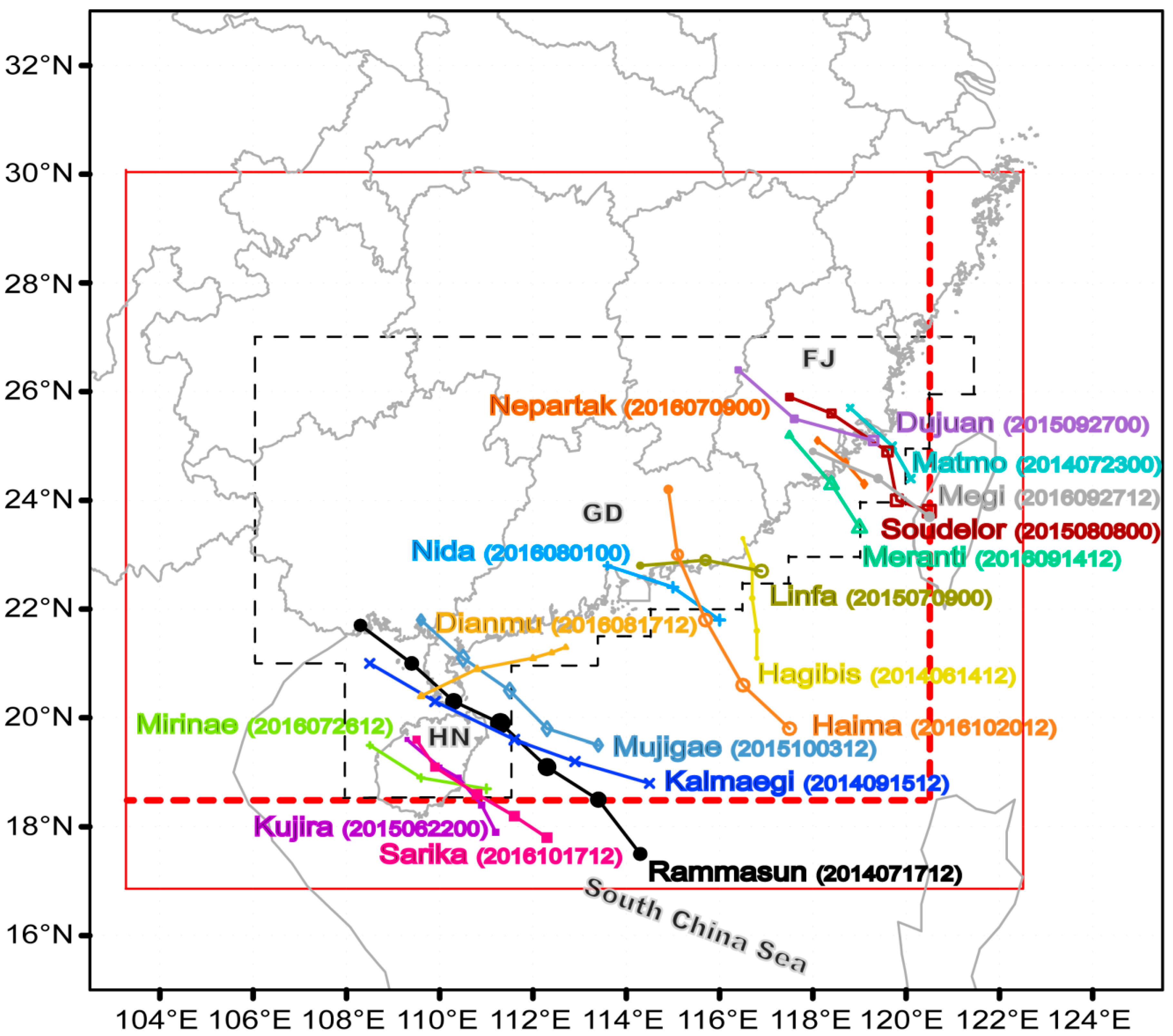
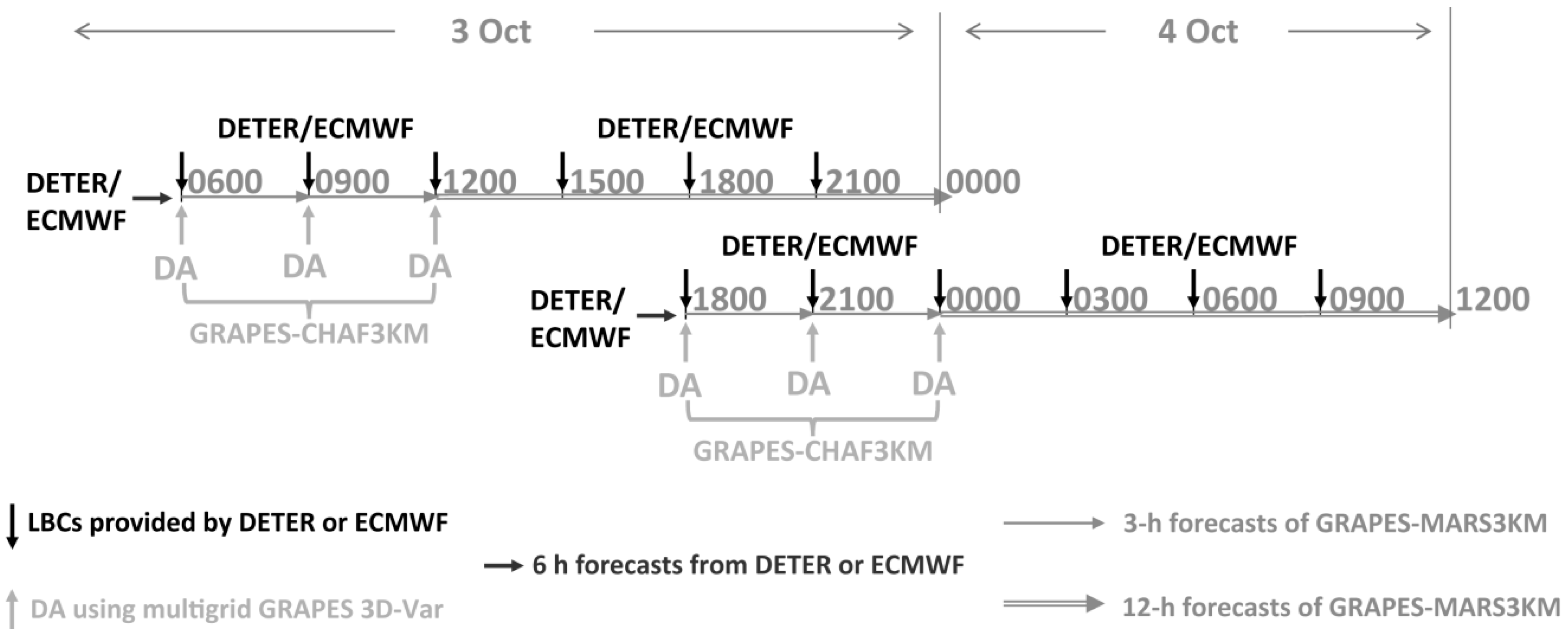

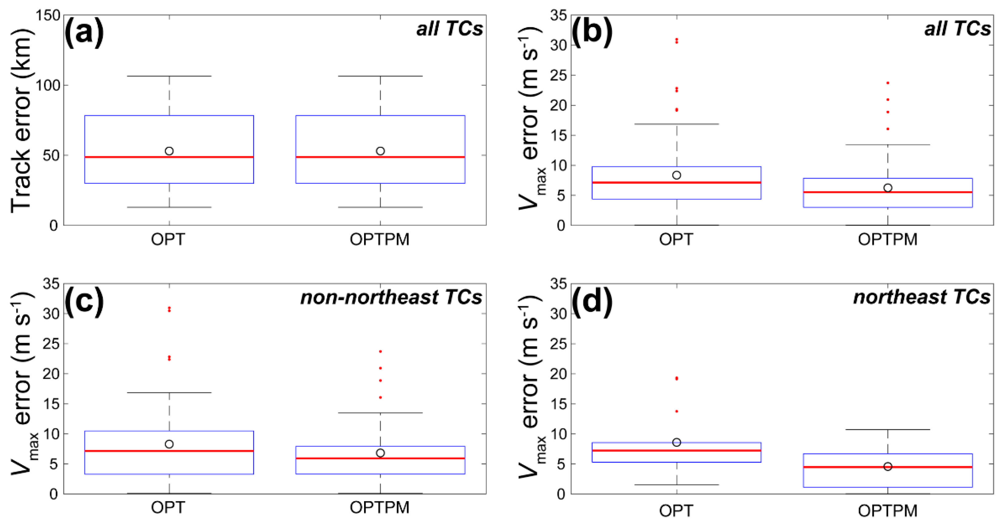
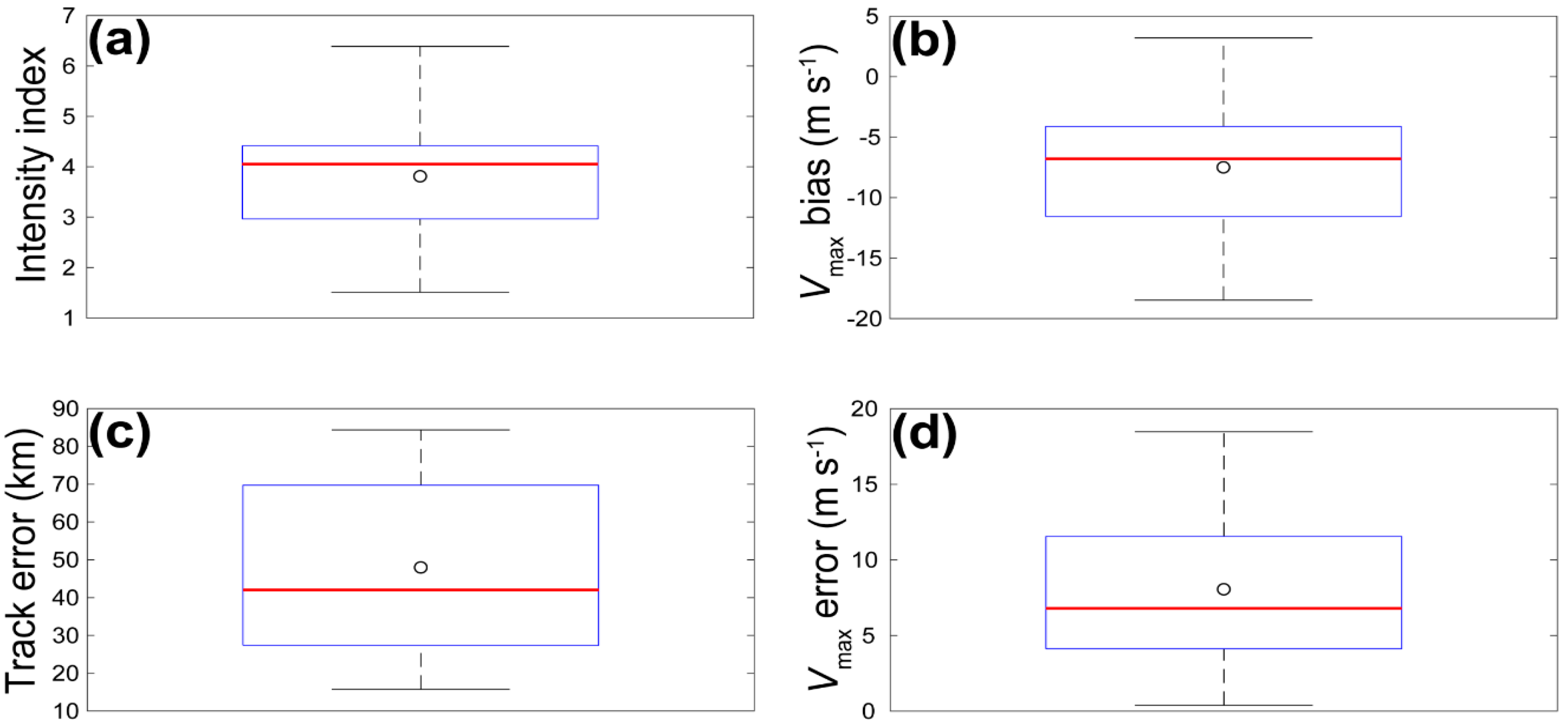
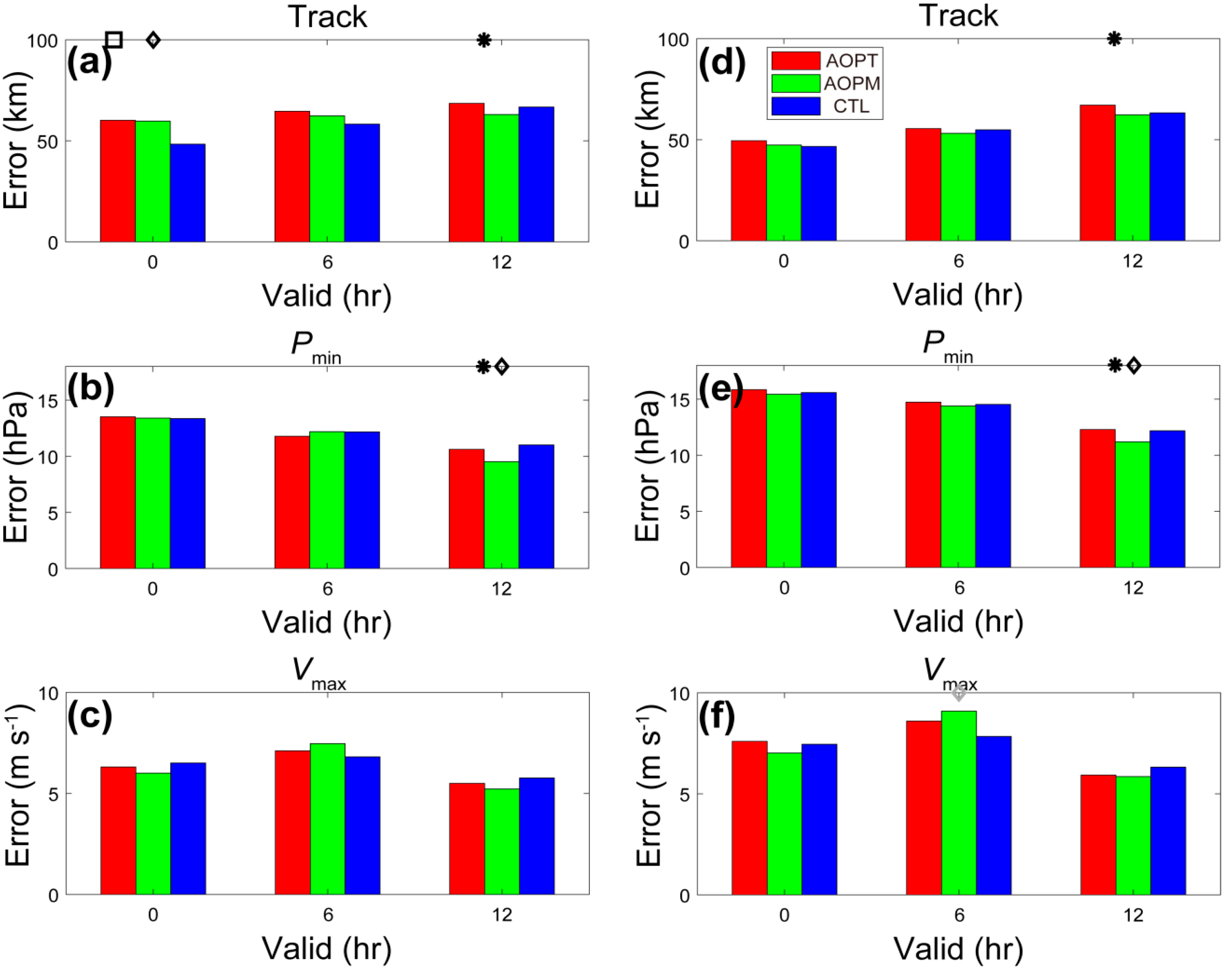
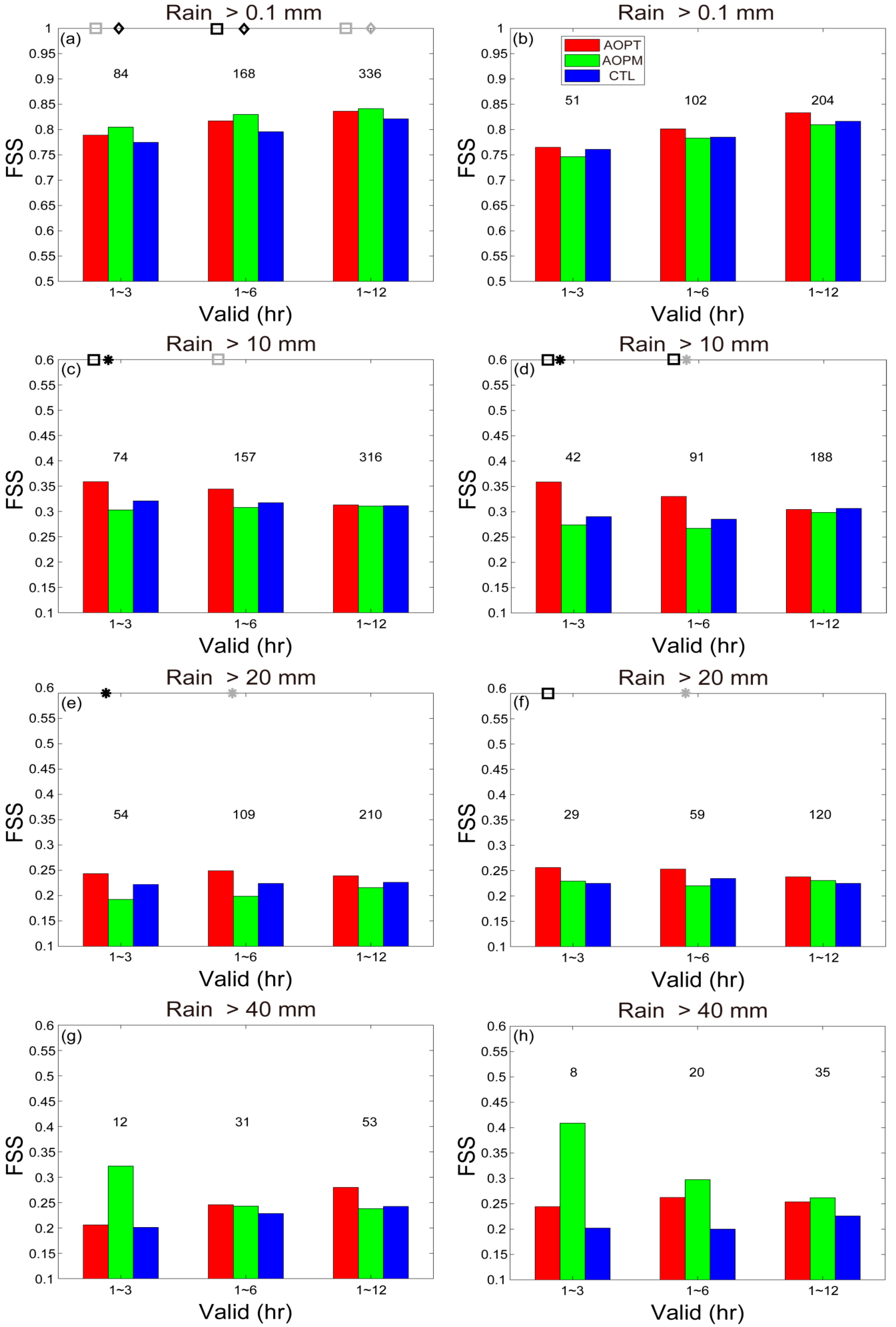
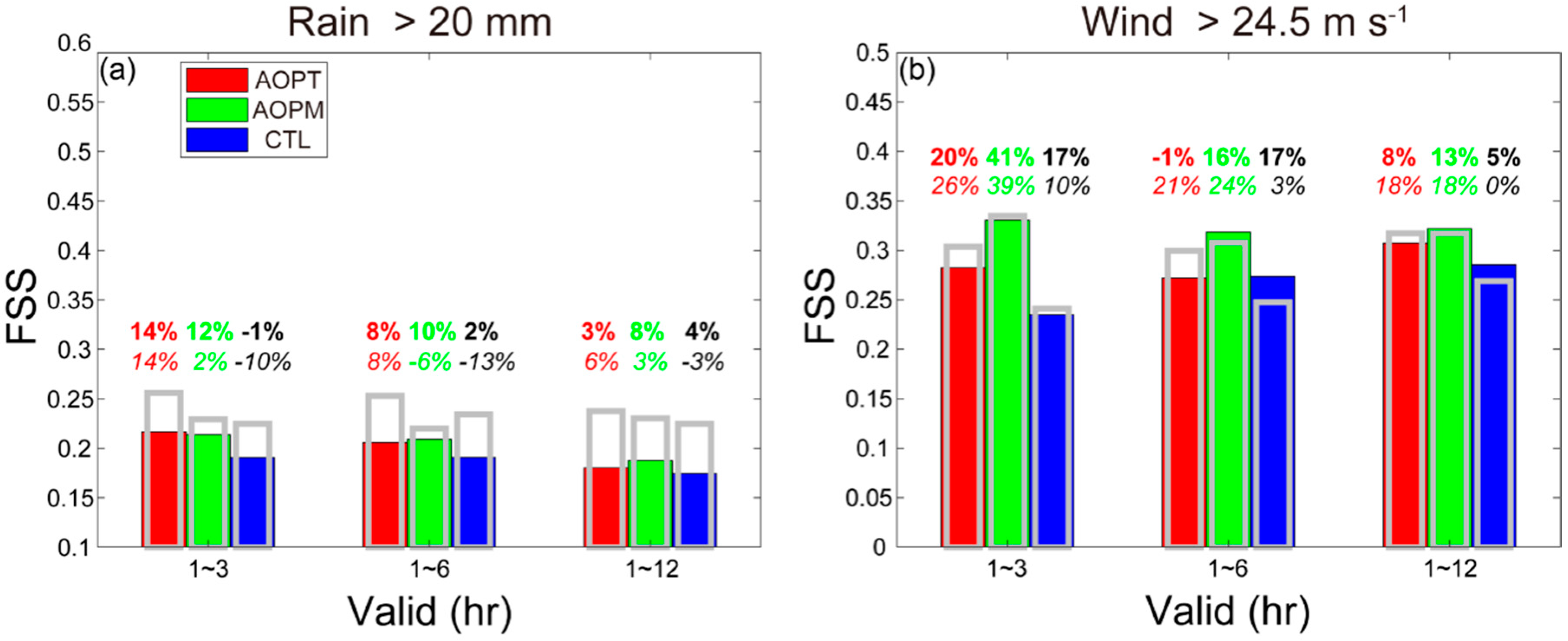
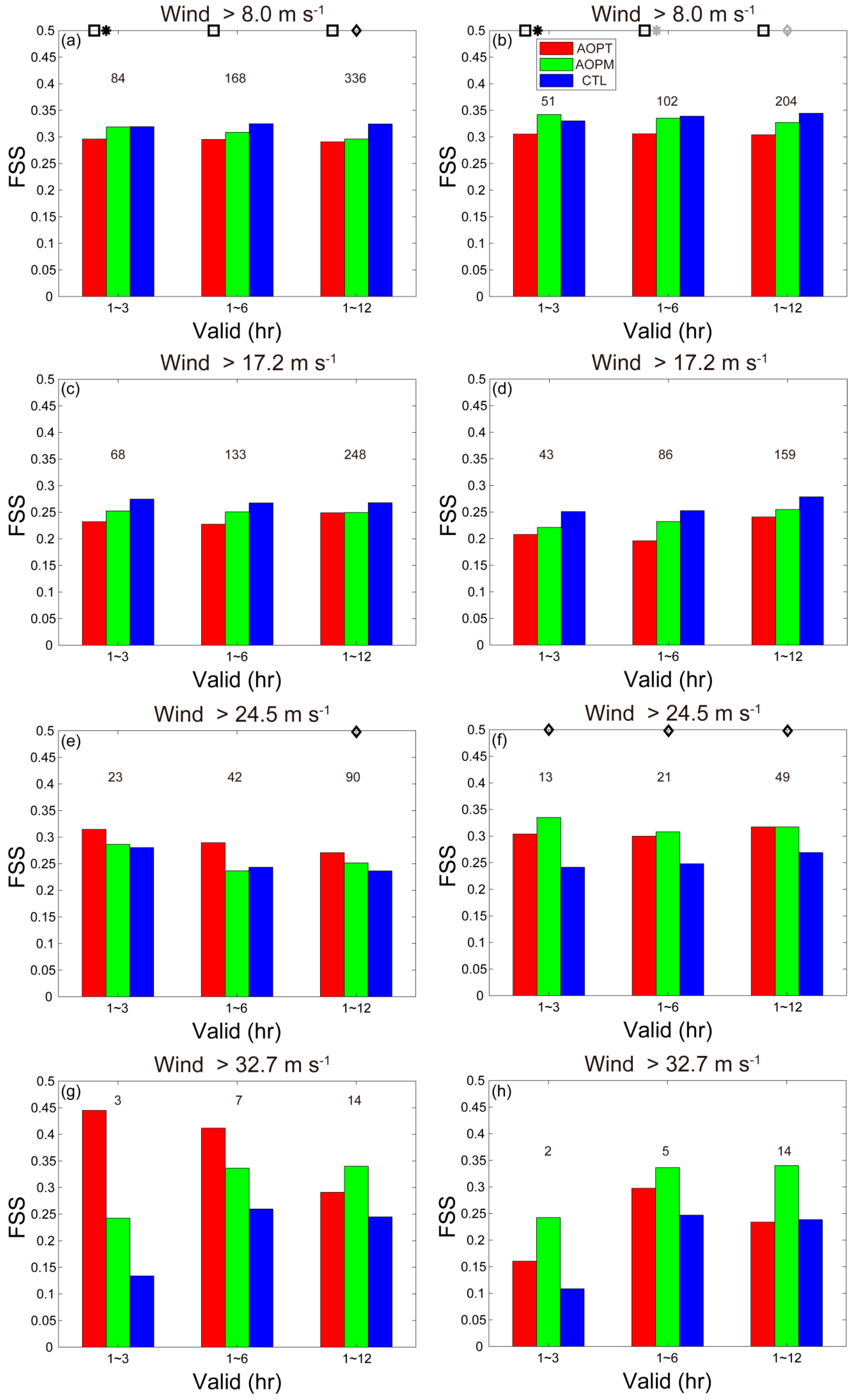
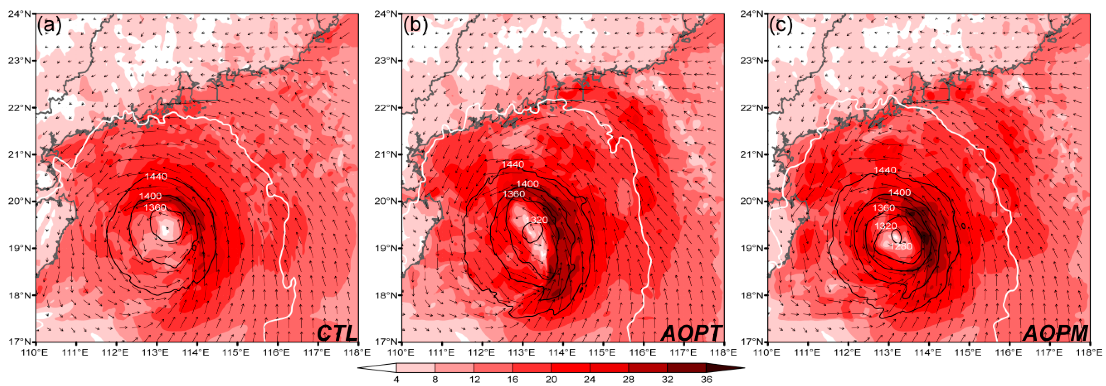
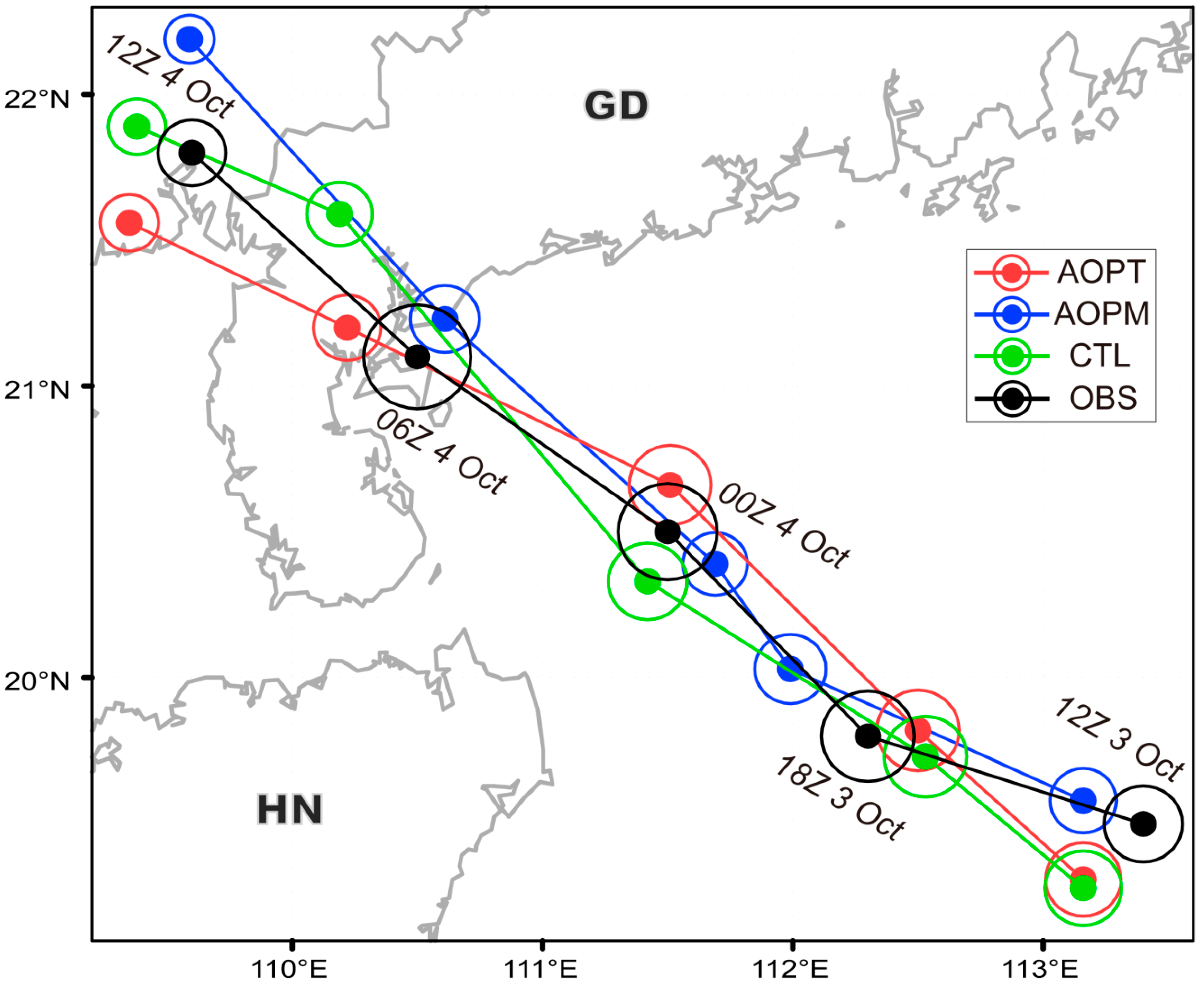

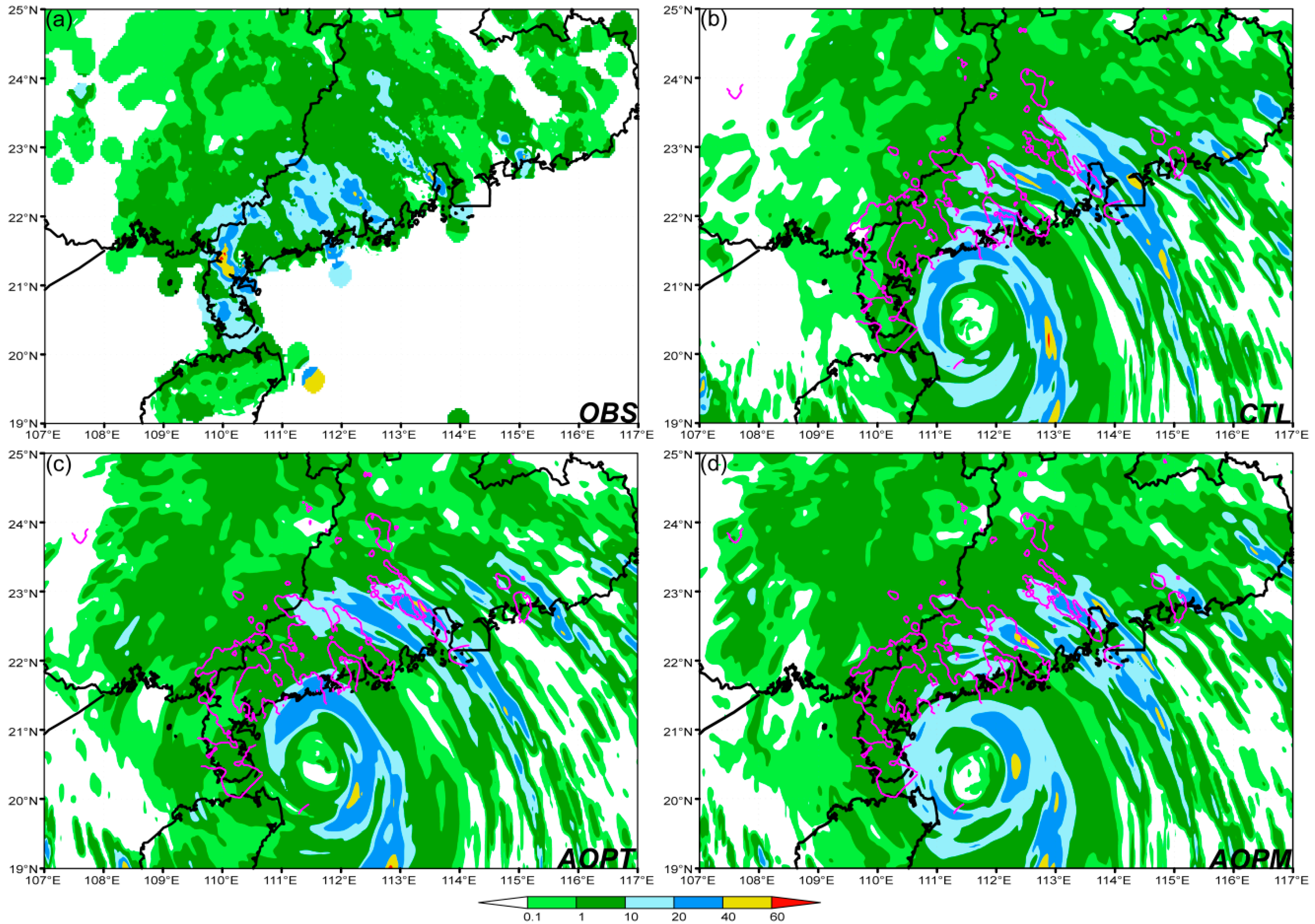
© 2019 by the authors. Licensee MDPI, Basel, Switzerland. This article is an open access article distributed under the terms and conditions of the Creative Commons Attribution (CC BY) license (http://creativecommons.org/licenses/by/4.0/).