Artificial Intelligence Based Ensemble Modeling for Multi-Station Prediction of Precipitation


1
Department of Water Resources Engineering, Faculty of Civil Engineering, University of Tabriz, Tabriz 51666, Iran
2
Faculty of Civil and Environmental Engineering, Near East University, Lefkoşa 99138, North Cyprus
3
Department of Computer Engineering, Faculty of Engineering, Near East University, Lefkoşa 99138, North Cyprus
4
Department of Electrical &Electronic Eng., Faculty of Engineering, Near East University, Lefkoşa 99138, North Cyprus
*
Author to whom correspondence should be addressed.
Atmosphere 2019, 10(2), 80; https://doi.org/10.3390/atmos10020080
Submission received: 3 January 2019
/
Revised: 31 January 2019
/
Accepted: 1 February 2019
/
Published: 15 February 2019
(This article belongs to the Special Issue Application of Machine Learning in Atmospheric Sciences and Climate Physics)
Abstract
:The aim of ensemble precipitation prediction in this paper was to achieve the best performance via artificial intelligence (AI) based modeling. In this way, ensemble AI based modeling was proposed for prediction of monthly precipitation with three different AI models (feed forward neural network-FFNN, adaptive neural fuzzy inference system-ANFIS and least square support vector machine-LSSVM) for the seven stations located in the Turkish Republic of Northern Cyprus (TRNC). Two scenarios were examined each having specific inputs set. The scenario 1 was developed for predicting each station’s precipitation through its own data at previous time steps while in scenario 2, the central station’s data were imposed into the models, in addition to each station’s data, as exogenous input. Afterwards, the ensemble modeling was generated to improve the performance of the precipitation predictions. To end this aim, two linear and one non-linear ensemble techniques were used and then the obtained outcomes were compared. In terms of efficiency measures, the averaging methods employing scenario 2 and non-linear ensemble method revealed higher prediction efficiency. Also, in terms of Skill score, non-linear neural ensemble method could enhance predicting efficiency up to 44% in the verification step.
1. Introduction
Precipitation is the most important component of the hydrological cycle and accurate prediction of precipitation plays critical roles in the design, planning and management of water resources and hydraulic structures. However, due to the complex, non-linear and stochastic nature of precipitation time series, its prediction is a quite difficult task.
The models for prediction of hydro-climate parameters (e.g., precipitation) are usually classified to 2 classes: physically based and black box models. The physically based model uses physical rules for modeling all of the proper physical processes involved in the precipitation procedure. On the other hand, black box models use historically observed data to make further estimations. Such black box methods are particularly developed on the basis of statistical and computational intelligence approaches. Although conceptual approaches are dependable methods to analyze the physics of the phenomena, they may show restrictions such as complexity, being time-consuming, and there being a lack of enough data for modeling; the physically-based models in comparison to black box models in comparison to black box models, deliver somewhat inaccurate results when there are not sufficient distributed information and data within the system. [1,2]. So, once the accurate estimations for the process are more crucial than the physical interpretations, utilizing data driven (black box) methods will be better alternative [2]. Recently, artificial intelligence (AI) methods as such black box methods showed great efficiency in modeling the dynamic precipitation process in the presence of the non-linearity, uncertainty, and irregularity of data. Comparative researches have shown that the AI-based models may generate reliable results in precipitation predictions with regard to the physically-based models [3,4]. It should be mentioned that the more accurate and sufficient data (long-term recorded data in terms of quantity and accurate recorded data in terms of quality) are available for calibrating the model, the obtained results will be more accurate and reliable in the long run. But due to the magnifying the prediction error over the next time steps of forecasting such data driven (AI-based) models are more accurate in short term forecasting issues. One of the most commonly used AI methods for the precipitation modeling is feed forward neural network (FFNN) which is a common type of artificial neural network (ANN). In the recent decades, FFNN has acquired increasing popularity due to its flexibility and robustness to detect involved patterns in the various range of data. For example, Guhathakurta [5] employed ANN for prediction of the monthly precipitation over 36 meteorological stations of India to estimate the monsoon precipitation of upcoming years. The model could catch non-linear interactions among input and output data and estimate the seasonal rainfall. Hung et al. [6] employed ANN for real time precipitation predicting and flood management in Bangkok, Thailand. It was found out that the most dominant input in modeling is rainfall at previous time steps (as a Markovian process). Likewise, Abbot and Marohasy [3] predicted monthly and seasonal precipitations up to 3 months in advance over Queensland, Australia, by using dynamic, recurrent and time-delay ANNs. More recently, Khalili et al. [7] employed the Hurst rescaled range statistical analysis to evaluate the predictability of the available data for monthly precipitation prediction for Mashhad City, Iran. Devi et al. [8] applied ANNs for forecasting the rainfall time series using the temporal and spatial rainfall intensity data and proved wavelet Elman models as the best model for rainfall forecasting. Mehdizadeh et al. [9] introduced two novel hybrid models of artificial neural networks-autoregressive conditional heteroscedasticity (ANN-ARCH) and gene expression programming-autoregressive conditional heteroscedasticity (GEP-ARCH) for forecasting monthly rainfall time series. They indicated that GEP-ARCH and ANN-ARCH methods could lead to reliable outcomes for the studied regions with different climatic conditions. They also revealed that ANN-ARCH method can present more reliable results with regard to GEP-ARCH method.
As another type of AI model, the least square support vector machine (LSSVM), first proposed by Ye and Xiong [10], is one of the most effective predicting methods as an alternative method of ANN. The LSSVM has been used for non-linear classification problems [11] and, function and density estimations [12]. The LSSVM is a machine learning algorithm to claim a model dealing with complicated classification problems. The LSSVM is capable of predicting non-linear, non-stationary, and stochastic processes [13]. The LSSVM has been successfully used for the prediction of precipitation in the last decade [14,15]. Lu and Wang [16] forecasted the monthly precipitation over a state in China employing LSSVM method using several kernel functions. Using the available observed data of 2 different stations from Turkey, Kisi and Cimen [17] employed the LSSVM with and without a wavelet-based data pre-processing technique for prediction of precipitation time series. Du et al. [18] employed an SVM-based precipitation forecasting method and reported the promising and effective results in the field of precipitation prediction. More recently, Danandeh Mehr et al. [19] developed a hybrid regression method on the basis of the support vector regression (SVR) and firefly algorithm (FFA) for precipitation prediction of rain gauges in Iran with promising accuracy. The outcomes revealed that the proposed combined method can significantly outperform the single SVR and GEP methods.
In addition to the ANN and LSSVM methods, the adaptive neural fuzzy inference system (ANFIS) model, which incorporates both the ANN learning power and fuzzy logic knowledge representation, has been considered as a robust model for precipitation prediction because of fuzzy concept ability in handling the uncertainty involved in the study processes [20]. ANFIS is a Takagi–Sugeno–Kang (TSK) fuzzy based mapping algorithm which provides less overshoot, oscillation and minimal training time [21]. The ANFIS can analyze the relationship involved in the input and output data sets via a training scheme to optimize the parameters of a given fuzzy inference system (FIS) [22]. The ANFIS training can use alternative algorithms to decrease the training error. Some previous investigations indicated that ANFIS can be used as an efficient tool for precipitation modeling (e.g., see, [23,24,25,26]). Yaseen et al. [27] employed a hybrid ANFIS-FFA model to forecast one month ahead precipitation value and compared the results with the classic ANFIS model. The results showed that, the proposed ANFIS-FFA method could perform more accurate than the classic ANFIS method, so that the efficiency of the ANFIS-FFA and ANFIS methods were strongly governed by size of the inputs set.
With the recent developments in the AI techniques, although ANN, ANFIS and LSSVM have been reliably employed to model time series of various hydro-climatic variables (including precipitation), it is obvious that for a particular problem, different outcomes may be obtained from different models over different spans of the time series. As such, Zhang [28] used a hybrid model of ANN and auto regressive integrated moving average (ARIMA) models for time series prediction, and suggested that the combination of the models is an effective way to increase prediction accuracy. Li and Sankarasubramanian [29] presented a new dynamic approach for combining multiple hydrological models evaluating the performance during prediction and also a weighted averaging method to reduce the modeling uncertainty in monthly streamflow prediction. Yamashkin et al. [30] confirmed that reliability, objectivity, and accuracy of the analysis are increased by the use of ensemble systems. Sharghi et al. [31] indicated that performance of the seepage modeling can be enhanced by the ensemble method up to 20%.
The ensemble precipitation prediction is a set of predictions that presents the range of rainfall prediction possibilities with a minimized error. The uncertainty associated with any prediction indicates that different scenarios are possible and the prediction must reflect them. By providing a range of possible outputs, the model shows how likely various scenarios come true in the months ahead, and which methods are useful and for how long they are useful for the future forecasts.
The main aim of this study is to utilize the models ensemble concept for precipitation prediction employing data from seven stations located in Turkish Republic of Northern Cyprus. The proposed ensemble techniques are formed using the outputs of the ANN, ANFIS, and LSSVM methods to improve the efficiency of single modeling. The three techniques of ensembling, which are simple, weighted and non-linear neural averaging, are applied in this way. Furthermore, two input combinations as scenarios 1 and 2, are considered for modeling with different input combinations. Although the ensemble approaches have been focused during the last decades at different engineering fields [28,32,33], to the best knowledge of the authors, this paper presents the first AI-based ensemble approach for precipitation prediction.
2. Experiments
2.1. Used Data and Efficiency Criteria
Cyprus is located at approximately 35° N and 33° E, in the east end of the Mediterranean Sea, and is ~224 km WSW to ENE, and ~97 km NNW–SSE with a land area of approximately 9250 km2 (Figure 1). The island has two mountain ranges—the Troodos Massif (maximum elevation 1951 m) in the southwest and the Pentadaktylos (Girne) range (maximum height 1000 m) along the northern coast, which give Cyprus high topographical variability [34].
The climate of North Cyprus is typical Mediterranean with hot dry summers where the average temperature can reach up to 40° C. In cool winter months the lowest temperature tends to be around 10° C.
Data from seven main stations (automatic sensors are usually used to measure the precipitation data in TRNC) were used in this study to predict the precipitation (see Figure 1). (1) Ercan International Airport; at this station, the summers are hot, arid, and clear and the winters are cold, windy, and mostly clear. Over the course of the year, the temperature typically varies from 4 °C to 35 °C and is rarely below 0 °C or above 37 °C; (2) Gazimağusa’s climate is classified as warm and temperate. In winter, there is much more rainfall in Gazimağusa than in summer. The average temperature in Gazimağusa is 19.3 °C and the average rainfall is 407 mm; (3) The prevailing climate in Geçitkale is known as a local steppe climate. During the year, there is little rainfall in Geçitkale and the average annual temperature is 19.1 °C; (4) Girne station’s climate is warm and temperate and the average annual rainfall is 382 mm. The winters are rainier than the summers. In Girne, the average annual temperature is 19.6 °C. Precipitation has an average of 449 mm; (5) Guzelyurt has a local steppe climate. There is little rainfall throughout the year. In Guzelyurt, the average annual values of temperature and precipitation are respectively 18.5 °C and 363 mm; (6) Lefkoşa has a hot semi-arid climate due to its low annual precipitation and annual temperature range. The city experiences long, hot, dry summers, and cool to mild winters, with most of the rainfall occurring in winter. The winter precipitation is occasionally accompanied by sleet and rarely by snow. The accumulation of snow is particularly rare (last events occurred in 1950, 1974, 1997, and 2015). There is occasionally light frost during the winter nights. The temperature reached 44.7 °C on 2 July 2017 in Lefkoşa; (7) Yeni Erenkoy’s climate is classified as warm and temperate. There is more rainfall in the winter than in the summer in Yeni Erenkoy. The average temperature in Yeni Erenkoy is 18.7 °C and about 520 mm of precipitation falls annually.
It should be mentioned that Automatic sensors are usually used to measure the precipitation data in TRNC which work with solar energy and battery system and precipitation is loaded into the data loggers and then data is collected with GPRS in every 15 minutes. Also the fine adjustment and calibration of the sensors are handled based on the international standards. The sensors’ accuracy and sensitivity are ±2% and 0.2 mm, respectively. Figure 2 shows the situation of rain gauge with the installation equipment. Also specifications of the rain gauges are tabulated in Table 1.
For training and validation of the models, the monthly data were obtained from these 7 meteorological stations for ten years, from 1 January 2007, to 31 December 2016. The characteristics of the stations and also the statistics of the data from stations are tabulated in Table 2.
Usually, as a conventional method, linear correlation coefficient (CC) is computed between potential inputs and output to select most dominant input variables for the AI methods such as FFNN [35]. However, implementation of CC for dominant input selection has been already criticized (e.g., see, [36]) since for modeling a non-linear process by a non-linear approach like FFNN, it will be more feasible to employ a non-linear criterion (e.g., mutual information (MI)) since in spite of a weak linear relation, strong non-linear relationships may be existing among input and output parameters. The MI value between random variables of X and Y can be written in the form of [37]:
where x and y are the probability distributions of variables X and Y; H(x) and H(y) show respectively the entropies of distributions x and y, and H(x,y) is their joint entropy as:
where PXY(x,y) is the joint distribution. The MI values between the observed precipitation time series of all seven stations relative to each other were calculated and tabulated in Table 3. As it can be seen from Table 3, overall, Ercan’s precipitation data are more non-linearly correlated with the precipitation time series of other stations, maybe due to its central position with regard to the others.
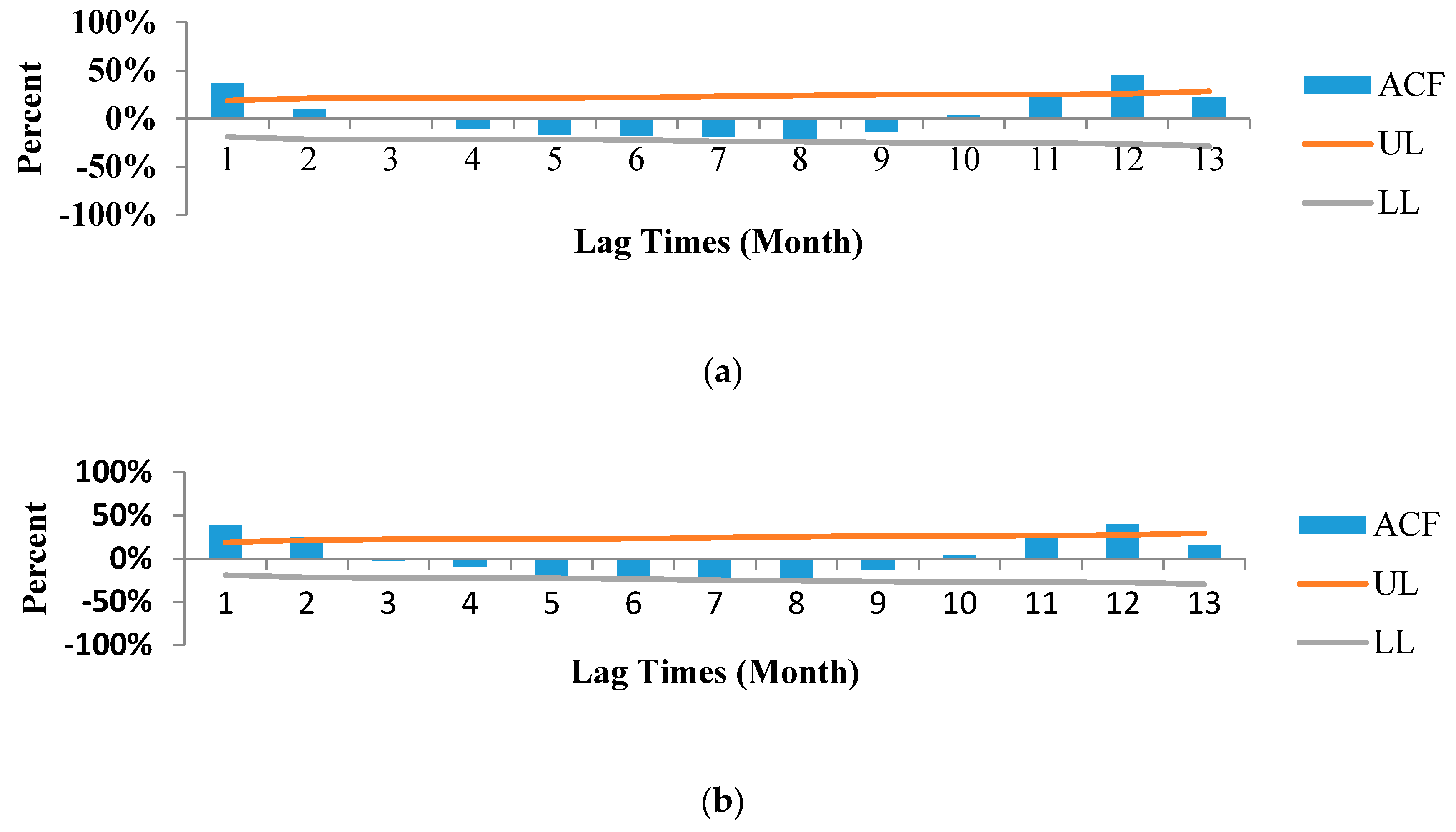
For instance, the auto-correlation function (ACF) plots (Correlogram) of Ercan and Lefkoşa precipitation time series are presented in Figure 3. As it can be seen from Figure 3, the precipitation time series of some stations such as Ercan station are more auto-correlated with 1 and 12-month lags, whereas the precipitation time series of some other stations such as Lefkoşa station are more auto-correlated with 1, 2, and 12-month lags. As noticed previously, CC is unable to recognize the non-linear relation between time series. Therefore, in continue the MI was employed to determine the non-linear relation between precipitation time series and their lag times. So, it was recognized that the precipitation time series are mostly correlated non-linearly with 1 and 12 month lags in all stations which denotes to both auto-regressive (Markovian) and seasonality of the process.
Beside computing auto-correlation function, for testing the normality of data, Kolmogorov Smirnov test [38] was used and results indicated that the data of all 7 stations are non-normal; so non-parametric tests should be applied to these datasets. Next, the Run test [39,40] was employed for testing randomness of precipitation time series of each station. Results of Run test at 95% confidence level indicated that precipitation of all stations are not random so that the precipitation of all stations are predictable. Also to check data homogeneity, Pettitt’s test [41], Standard normal homogeneity test (SNHT) [42], Buishand’s test [43] and Chi-square test [44] were applied to data of all stations which probed that data of stations are homogenous.
Prior to the modeling, the monthly average precipitation data were first normalized by [45]:
where Pnorm is the normalized value of the P(t); Pmax(t) and Pmin(t) are the max and min values of the observed data, respectively. For training and verifying purposes, the data were divided to 2 sub-sets. About 70% of whole data were used for calibration and the rest 30% of data were used for verifying the trained methods.
The “root mean square error (RMSE)” and “determination coefficient (DC)” were used to evaluate the prediction efficiency of the models as [46]:
where n is the data number, Pobsi is the observed data, and Pcomi is the predicted (computed) data. DC ranges from −∞ to 1 with a perfect score of 1 and RMSE ranges from 0 to +∞ with the perfect value of 0. Legates and McCabe [47] showed that any hydro-environmental method may be adequately evaluated by DC and RMSE criteria.
Also the “Skill” of the proposed methodology was calculated as [48]:
where A is the measure of accuracy (such as RMSE or DC), Aref is the set of reference predictions and Aperf is a perfect prediction (what actually happened). Skill scores have a range of (∞,1], where a score of 1 presents perfect model performance, a score of 0 means the model is as accurate as the reference model, and a negative score means the model is less accurate than the reference.
2.2. Proposed Methodology
In this study, firstly, the monthly precipitation data were normalized by Equation (3). Three different black box models, ANN (a commonly used AI method), ANFIS (an AI method which serves Fuzzy tools to handle the uncertainties involved in the process) and LSSVM (more recently developed AI model), were separately created on the basis of two different scenarios. Then, outputs of the single models were ensembled using 3 ensemble techniques as linear simple and weighted averaging and non-linear neural ensemble methods. The inputs of the ensemble unit were outputs of the single models. The modeling was done via two scenarios. In scenario 1, each station’s own data at previous time steps were used for predicting the same station’s precipitation at current time step, while in scenario 2, another station’s data in addition to each station’s data were used for modeling to enhance the prediction performance.
2.2.1. First Scenario
For modeling via the first scenario, the aim was to predict precipitation value using its values at previous time steps. So, the prediction of the precipitation could be patterned as:
i denotes to the station name (as Ercan, Gazimağusa, Geçitkale, Girne, Guzelyurt, Lefkoşa and Yeni Erenkoy stations) and are the precipitation values of ith station corresponding to time steps t−1 and t−12 (or 1 and 12 months ago).
The conceptual model of the ensemble system for scenario 1 involving ANN, ANFIS and LSSVM single models is shown by Figure 4.
P(t−1) and P(t−12) are previous monthly precipitation values corresponding to 1 and 12 months ago; PFFNN(t), PANFIS(t) and PLSSVM(t) are results of predictions (in current month) by different models. The argumentation of using P(t−1) and P(t−12) as inputs for prediction of P(t) is supported by the following:
(a) As shown by some previous studies [3,6,27] in modeling precipitation, as a Markovian (auto-regression) process, P(t) is more correlated with precipitation values at prior time steps as P(t−1) and so on. For this reason, it is feasible to select previous time steps values as inputs for the AI models. According to Figure 3a,b, and also employing MI, as a non-linear correlating identifier, the lag times of 1 was selected as the dominant input in scenario 1 for all stations.
(b) Selection of input P(t−12) is related to the seasonality of the precipitation phenomenon. It means that due to the seasonality of the process (i.e., periodicity), the precipitation value of the current month has a strong relation (similarity) with the precipitation level in the same month at previous year. As it can be seen in Figure 3a,b, the precipitation is much correlated with the precipitation values with the values obtained 12 months ago. It should be noted that the CC could determine the linear correlation between two time series and it is unable to recognize the non-linear relation. Hence, MI was used to confirm the selection of dominant inputs for the modeling.
2.2.2. Second Scenario
In scenario 2, the prediction formula (7) was modified by introducing precipitation value from Ercan station as exogenous input. So, the following equation could be considered to formulate this scenario:
In scenario 2, it was tried to use the data from another station as exogenous inputs to enhance the modeling efficiency. In this way, the data from Ercan station were also considered as input data for modeling all other stations. This was due to the fact that the position of Ercan station is central in comparison to the other stations and therefore has more non-linear correlation with other stations (see Table 3). Also, the location of this station is of vital importance as it is the main airport of TRNC, so the data obtained from here may be more accurate and complete. Thus, the data obtained from the Ercan station were considered as exogenous input in the modeling via scenario 2.
Employing scenario 2 can be more helpful for predicting the precipitation of stations when they get out of service (due to technical problems) using their available past observations as well as data from Ercan station.
2.3. Feed Forward Neural Network (FFNN) Concept
The artificial neural network as an AI-based model is a mathematical model aiming to handle non-linear relationship of input-output data set [49]. ANN has proved to be effective with regards to complex function in various fields, including prediction, pattern recognition, classification, forecasting, control system and simulation [50,51]. Among the different ANN algorithms, FFNN with back propagation (BP) training is widely applied and is the most common class of ANNs. In FFNN-BP, the network is trained by processing the input data through the network and it is transferred to the output layer, and the generated error propagated back to the network until the desired output is archived. The primarily strategy of FFNN-BP is to reduce the error, so that the ANN is trained by the training data set and can predict the correct output [52]. FFNN includes 3 layers of input, hidden and output.
In this study, the input layer consisted of combinations of P(t−1), P(t−12) and the target was P(t) as shown in Figure 5. Both the architecture (the number of neurons, number of layers, transfer function) and learning rate is usually determined using the trial-and error process. The sigmoid activation function was employed for input and hidden layers while in the output layer, a linear function was applied in the used FFNN models [53]. The developed ANN structure is illustrated by Figure 5.
2.4. Adaptive Neural Fuzzy Inference System (ANFIS) concept
The conjunction of ANN and fuzzy system presents a robust hybrid system which is capable of solving complex nature of the relationships [21,54]. ANFIS is a multi-layer feed-forward (MLFF) neural network that is capable of integrating the knowledge of ANN and fuzzy logic algorithms which maps the set of inputs to the outputs [51]. ANFIS as AI-based model employs the hybrid training algorithms which consist of a combination of BP and least squares method [55]. In addition, in terms of learning duration, the ANFIS model is very short in comparison with the ANN model [53]. The schematic of the ANFIS model is depicted by Figure 6.
The developed ANFIS consists of two inputs of P(t−1), P(t−12) and one output of P(t) as shown in Figure 6. Among different FISs used as fuzzy operations, the TSK engine was used in this study. The operation of ANFIS to generate the output function with 2 input vectors of P(t−1), P(t−12) and the first order of TSK applied to 2 fuzzy rules can be expressed as [26]:
Rule (1): if µ(P(t−1)) is B1 and µ(P(t−12)) is C1 then f1=p1(P(t−1)) + q1(P(t−12)) + r1
Rule (2): if µ(P(t−1)) is B2 and µ(P(t−12)) is C2 then f1=p2(P(t−1)) + q2(P(t−12)) + r2
B1, B2, and C1, C2 are membership functions parameters, for inputs P(t−1) and P(t−12) and p1, q1, r1 and p2, q2, r2 are outlet functions’ variables, the structure and formulation of ANFIS follows a five-layer neural network structure. For more explanation of ANFIS, the reader is referred to the studies of [20,25].
2.5. Least Square Support Vector Machine (LSSVM) concept
Learning in the context of SVM was proposed and introduced by [56], which provides a satisfactory approach to the problems of prediction, classification, regression and pattern recognition. SVM is based on the concept of machine learning which consists of data-driven model [56]. The structural risk minimization and statistical learning theory are two useful functions of SVM which make it different from ANN because of its ability to reduce the error, and complexity and increases the generalization performance of the network. Generally, SVM is categorized into linear support vector regression (L-SVM) and non-linear support vector regression (N-SVM) [57]. Therefore, support vector regression (SVM) is a form of SVM based on two basic structural layers; the first layer is kernel function weighting on the input variable while the second function is the weighted sum of kernel outputs [56]. In SVM, firstly a linear function should fit to data and thereafter, the outcomes are passed through a non-linear kernel function to map non-linear patterns involved in data. The least squares formulation of SVM is called LSSVM. Thus, the solution in this method is obtained through solving a linear equations system. Efficient algorithms can be used in LSSVM [58]. In LSSVN modeling a non-linear function can be expressed in the form of [59]:
in which f shows relation among the input and output data, w is an m-dimensional weight vector, ϕ denotes to kernel function mapping input vector x to an m-dimensional feature vector; b stands for the bias [14]. The regression problem can be given as follows [10]:
which has the following constraints:
where γ is the margin parameter and ei is the slack variable for Xi. To solve the optimization problem, the objective function may be achieved by altering the constraint problem to the unconstraint problem, according to the Lagrange multiplier α_i as [60]:
Vector w in Equation (9) should be calculated after solution of the optimization problem in the form of [16]:
Therefore, the ultimate formula for LSSVM could be written in the form of:
where P(x,xi) shows kernel function which performs non-linear mapping to the feature space. The Gaussian radial basis function (RBF) is the most commonly used kernel function in LSSVM based modeling in the form of [23]:
where γ and σ are the parameters of the kernel function. Figure 7 shows the structure of the LSSVM.
2.6. Ensemble Unit
In the case that various models have better results at different parts or intervals or in modeling of peak values, it is supposed that by combining (ensembling) the outputs from several prediction methods, the final accuracy of a predicted time series can be improved. In an ensembling process, the outcomes of various models are used and as so, the final outputs will not be sensitive to selection of the best methods. Therefore, predicts of ensemble method will be more safe and less risky than the results of the single best methods. Various studies at different fields of engineering suggested to ensemble outcomes of several methods as an effective approach to improve the performance of time series predictions [32,61].
An ensemble technique, as a learning algorithm, gathers a set of classifiers to classify new variables by applying weights on the single prediction values. The goal of such ensemble learning technique is to develop an ensemble of the individual methods that are diverse and yet accurate.
In current paper, 3 ensemble techniques were applied to combine of the outputs from the used AI-based models to enhance the overall efficiency of the predictions as:
(a) the simple linear averaging method:
In which shows the outcome of simple ensemble method. N shows the number of used models (in this study, N=3) and stands for the outcome of the ith method (i.e., ANN, ANFIS and LSSVM) in time step t.
(b) the linear weighted averaging method:
where i shows imposed weight on the output of ith method and it may be computed on the basis of the performance measure of ith method as:
where DCi measures the model efficiency (such as coefficient of determination).
(c) the non-linear neural ensemble method:
For the non-linear neural ensemble method another FFNN model is trained by feeding the outputs of single AI models as inputs to the neurons of the input layer (see Figure 8). Number of hidden layer neurons and maximum epoch numbers are defined through trial-error procedure.
3. Results and Discussion
In this section, firstly obtained results of sole models are presented and then the results of the ensemble methods are summarized.
3.1. Results of Single AI Models
At the first step, FFNN, ANFIS, and LSSVM models were separately created via the proposed scenarios 1 and 2. For precipitation prediction of the stations, monthly precipitation values were individually imposed into ANN, ANFIS, and LSSVM models in order to predict one-month-ahead precipitation. For this purpose, the ANN, ANFIS, and LSSVM models’ architectures set depends on the priority of the precipitation process. The monthly precipitation data are described by both Markovian and seasonal properties [13]. For this reason, the current precipitation P(t) is related to its previous time steps, P(t−1), as well as the its value at twelve months ago, P(t−12). Consequently, the input values as P(t−1) and P(t−12) were applied to the FFNN, ANFIS, and LSSVM models to predict precipitation at time step t (P(t)) for scenario 1 (including more lagged precipitation values, i.e., P(t−2) and P(t−3) did not show higher MI with output and could not improve the efficiency of the modeling). For scenario 2, one more input, Ercan’s station precipitation value as exogenous input, was also considered (in addition to the input of scenario 1) as another input neuron to enhance the prediction performance (Ercan station’s precipitation at time step t−1 and t−2 was also examined as exogenous inputs but it couldn’t improve the modeling efficiency remarkably and so, only the value at time step t was used in modeling).
To prevent the FFNNs from overtraining issue, it is important to select optimum number of hidden neurons as well as training iteration (epoch) number. Levenberg Marquardt algorithm [62] as training algorithm and 10–300 training epoch numbers and 1–30 hidden neurons were examined to develop the FFNN models. The best results by FFNN models for precipitation modeling of all stations are shown in Table 4 for both scenarios 1 and 2.
To train the ANFIS models, the Sugeno FIS engine was used in the modeling framework. Each ANFIS should include some rules and membership functions. In this research, Gaussian-shaped and 2 Gaussian combinations MFs, as well as the Triangular-shaped and pi-shaped MFs were found to be appropriate for monthly precipitation modeling. Furthermore, the constant MF was applied in the output layer of the ANFIS models. Not only the number of membership functions but also the number of training epochs were examined to reach to the optimum ANFIS models. The ranges of 5–300 and 2–5 were considered respectively for the numbers of training epoch and membership functions. The best results for the ANFIS models are shown in Table 5 for all stations obtained via both scenarios 1 and 2.
Thereafter, the LSSVM models were created to predict the precipitation time series of the stations using RBF kernel. Several studies have already reported more reliable results of LSSVM model using RBF kernel with regard to using other kernels maybe due to its smoothness assumption [59]. The best results obtained by LSSVM in modeling the precipitation of the stations are shown in Table 6 for both scenarios 1 and 2.
As it is shown by Table 4, Table 5 and Table 6, the results of the methods in scenario 1 show a bit better performance for Ercan and Lefkoşa stations than other stations in the verification phase since these stations are located in central and higher parts of the island in contrast to the other stations which are located in shore lines and are impacted more significantly by the irregular variations of the sea condition such as stormy or calm sea conditions. This can also be confirmed by the standard variation values presented in Table 2 which show lower values for these two stations.
In scenario 2, the models of the Girne station in verification step showed better efficiency than others. This can be due to its proximity to Ercan station. In other words, not only the small distance between Girne and Ercan stations but also the predominant wind direction over the island (which is from northwest to southeast) make the precipitation pattern of both stations more similar with regard to the others. It should be noted that other factors also influence the precipitation pattern but, since Cyprus is a small island and most of the conditions do not vary part to part; so it supposed that the wind may be the main factor. This can also be clearly seen from Table 3 which shows higher MI value between these two stations.
Considering the outcomes of both scenarios, because of using Ercan station’s data as exogenous input (in addition to each station’s own data), the results of scenario 2 were better than scenario 1, showing improvement of modeling efficiency up to 61% via ANFIS model for Gazimağusa station in calibration step and up to 58% via LSSVM model for Güzelyurt station in verification step.
For instance, Figure 9, Figure 10 and Figure 11 illustrate the results of single AI methods for the calibration and verification steps and scatter plots for verification step for Ercan and Girne stations based on scenarios 1 and 2, respectively.
As it can be seen from Table 4, Table 5 and Table 6 and Figure 9, Figure 10 and Figure 11, generally in most cases, the performance of FFNN was better than other models, however in some cases, the ANFIS and in some other cases LSSVM’s performance was better than others. Also, comparison of the outputs obtained by the single AI methods (Figure 9, Figure 10 and Figure 11) shows that in different parts of the time series, some of the models led to over estimations and others down estimations of the observed time series. Figure 9a highlights 2 points (i) and (ii). According to the figure, it is obvious that for the point (i), LSSVM method provided better fitting to the observed value. However, for sample point (ii), the FFNN model led to the minimum error. In addition, in the interval of November- 2009 to March- 2010 and November- 2012 to January- 2013, all models were unable to provide good predictions. Therefore, such different performances of different methods at different sample points and time spans confirm a need to ensemble the results of different methods via the ensemble techniques.
3.2. Results of Ensemble Modeling
In the ensemble modeling, the outputs of three AI based single models were combined to improve the predicting performance. In this step, only the verification dataset was employed to compute the weights of the averaging methods. For the neural averaging method, like the single FFNN model, the Levenberg Marquardt algorithm was used as training algorithm. The ranges of 10–300 and 1–30 respectively for the numbers of training epochs and hidden neurons were examined to obtain the best results. Results of different ensemble methods are shown by Table 7 and Table 8 respectively for scenarios 1 and 2. Also the Skill scores of ensemble methods with regard to classic single AI methods are tabulated in Table 9.
The outputs obtained by the ensemble techniques indicate that almost all three ensemble techniques could produce reliable results in comparison to the single AI methods.
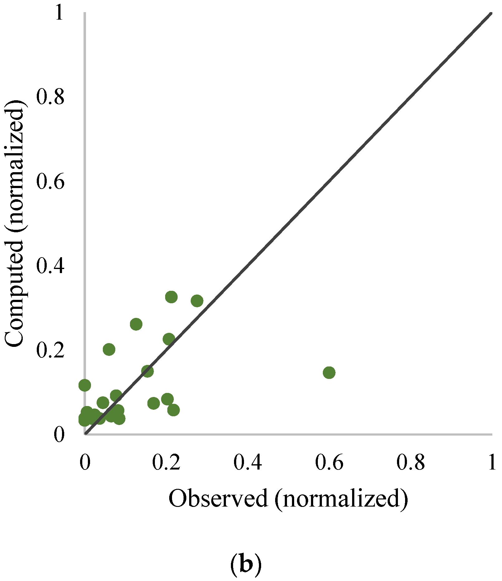
For example, Figure 12 shows the results of precipitation predictions using the ensemble models for both calibration and verification phases and the scatter plot for the verification step by using the neural ensemble method for Girne station based on the second scenario.
As mentioned above, any method has its own benefits and drawbacks. Some models may provide over and some others may provide lower estimates. Also each model could estimate specific intervals more accurate than other models. Thus, by combining outputs of different methods the final estimations may be more accurate in comparison with the results of single models. It should be noticed that since the outputs of the single methods are close together (see Table 4, Table 5 and Table 6), and because the efficiency of simple and weighted averaging ensemble techniques are in the same directs with the single methods, outputs of simple and weighted ensemble techniques are quite same. As it can be seen in Table 7 and Table 8 and Figure 12, the efficiency of neural ensemble is better than the linear ensembling methods in the most cases.
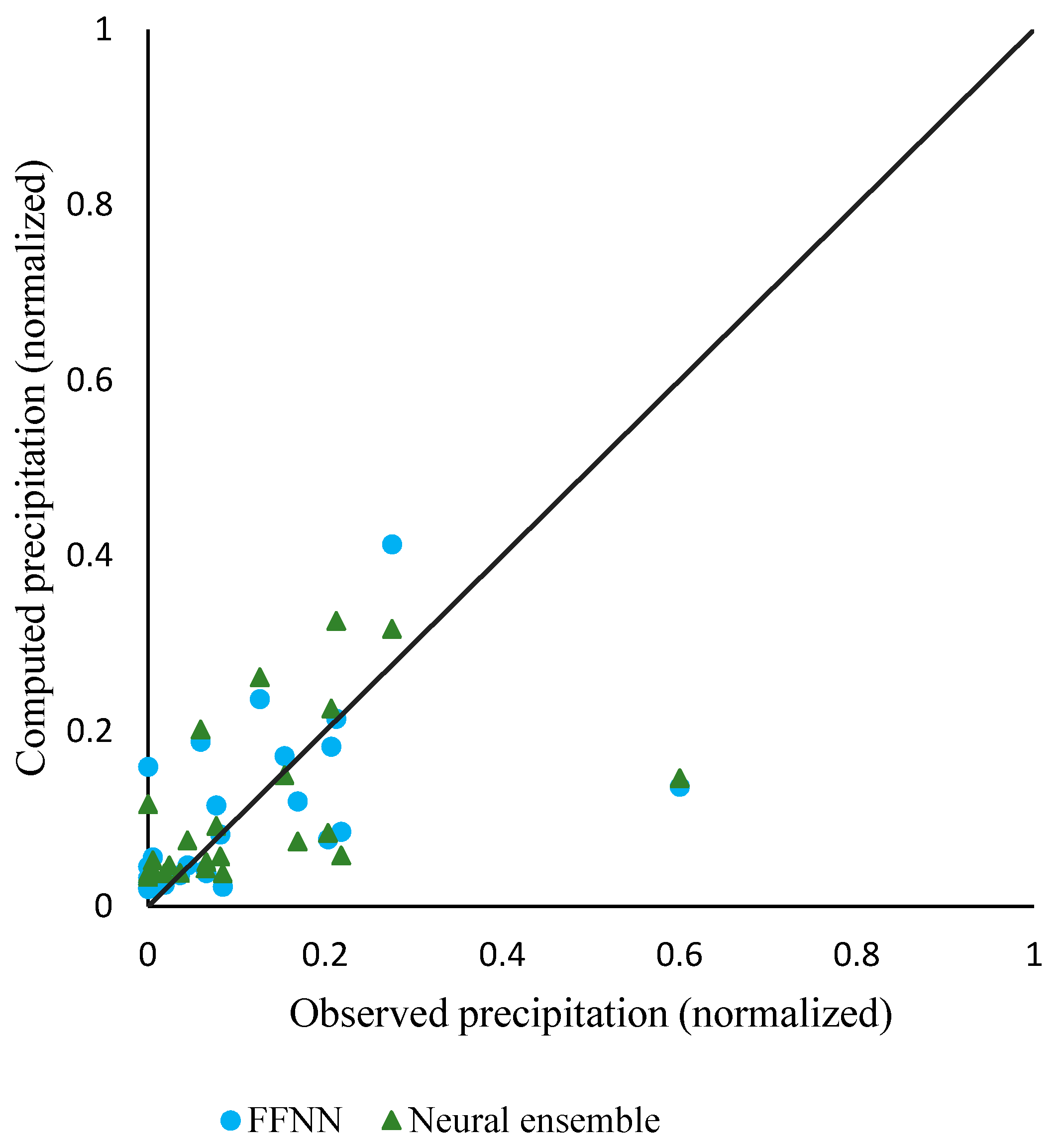
For instance, the scatter plot of FFNN and neural ensemble methods based on scenario 2 for Girne station at verification step is presented by Figure 13.
In terms of computed DC and Skill measures (see Table 4, Table 5, Table 6, Table 7, Table 8 and Table 9), simple linear, weighted linear and neural averaging methods enhanced the predicting performance up to 26.33% in Güzelyurt station relative to ANFIS, 25.33% in Güzelyurt station relative to ANFIS, 47.68% in Ercan station relative to ANFIS and 54.74% in Lefkoşa station relative to FFNN, 50% in Lefkoşa station relative to FFNN, 79.74% in Lefkoşa station relative to FFNN in calibration step for scenarios 1 and 2 and up to 32.3% in Geçitkale station relative to ANFIS, 32.5% in Geçitkale station relative to ANFIS, 36.17% in Geçitkale station relative to ANFIS and 19.06% in Yeni Erenköy station relative to ANFIS, 20.5% in Girne station relative to ANFIS, 44.39% in Yeni Erenköy station relative to ANFIS in verification step for scenarios 1 and 2, respectively. It is obvious that the neural ensemble could lead to better results by 65% on average. Furthermore, the ensembling model could improve the efficiency of precipitation modeling of Yeni Erenköy station more than other stations by 21% on average in the verification step. On the other hand, this method could not improve the modeling efficiency of Gazimağusa station meaningfully.
4. Conclusions
In this paper, AI based ensemble method was used to increase the precision of monthly precipitation prediction. The FFNN, ANFIS, and LSSVM predictors were developed on the precipitation data from seven stations in North Cyprus. Thereafter, the ensemble methods, based on linear (simple and weighted averaging) and non-linear (FFNN based) averaging methods were employed to increase the modeling efficiency.
Two scenarios were considered with different input variables that in scenario 1, each station’s own pervious data were used for modeling while in scenario 2, the central station’s (Ercan station) data were also employed in addition to each station’s own data. The results of two employed scenarios indicated that scenario 2 had better performance and could enhance the modeling efficiency up to 58%, in the verification step because of employing the observed data from the Ercan station as exogenous input in simulating other stations’ precipitation.
Among three single AI models, the FFNN model showed better performance in most cases in the verification step.
Analysis of the results in terms of computed DC, RMSE, and Skill values show that the ensemble methods provide better results with regard to the single AI-based methods. Furthermore, the ensemble model based on the non-linear averaging produced better predictions than the single models and linear ensemble models up to 80% and 44% for calibration and verification steps respectively.
Due to the black box inherit of the proposed methodology in this paper, it is clear that although the method can be similarly applied to other case studies, the models must be again calibrated using the data from the new cases and consequently the modeling may lead to a bit different outcomes. Furthermore, the method was applied to the available data in this study, but due to the flexibility of the method, in the case of obtaining more new data, the results can be easily up-dated. One of the limitations of the considered ensembling methods in this study is that they statically average the outputs of the AI models for all time steps. With this regard, and as a research plan for future, it is useful to further increase the performance of the ensemble model by dynamic and adaptive selection of outputs of single AI-based models in terms of the minimum error of approximations. Also, some other AI based methods may also be used in the ensemble unit in addition or instead of the used methods (i.e., FFNN, ANFIS and LSSVM).
Author Contributions
Formal analysis, S.U.; Project administration, F.S.; Supervision, V.N.; Writing–original draft, N.B.
Funding
This research received no external funding.
Conflicts of Interest
The authors declare no conflict of interest.
Nomenclature
| Symbol | Description |
| A | measure of accuracy |
| B | membership functions parameter |
| b | bias |
| C | membership functions parameter |
| ei | slack variable |
| H(X) | entropy of X |
| H(X,Y) | joint entropy of X and Y |
| N | number of single models |
| n | data number |
| p | outlet function variable |
| Pobs | monthly observed precipitation (mm/month) |
| Pcom | monthly calculated precipitation (mm/month) |
| P(max)t | max value of monthly observed precipitation (mm/month) |
| P(min)t | min value of monthly observed precipitation (mm/month) |
| Pnorm | normalized value of monthly observed precipitation |
| Pi(t) | precipitation of station i at time t (mm/month) |
| P(t-α) | previous monthly precipitation value corresponding to α moth ago (mm/month) |
| PErcan(t) | monthly precipitation of Ercan station at time t (mm/month) |
| P(t) | precipitation monthly data (mm/month) |
| q | outlet function variable |
| r | outlet function variable |
| t | time (month) |
| w | weight |
| α | Lagrange multiplier |
| ɣ | margin parameter |
| λ | kernel parameter |
| ϕ | kernel function |
References
- Nourani, V.; Mano, A. Semi-distributed flood runoff model at the sub continental scale for southwestern Iran. Hydrol. Process. 2007, 21, 3173–3180. [Google Scholar] [CrossRef]
- Clarke, R.T. Statistical Modelling in Hydrology; John Wiley and Sons: Hoboken, NJ, USA, 1994; p. 412. [Google Scholar]
- Abbot, J.; Marohasy, J. Application of artificial neural networks to rainfall forecasting in Queensland, Australia. Adv. Atmos. Sci. 2012, 29, 717–730. [Google Scholar] [CrossRef]
- Jiao, G.; Guo, T.; Ding, Y. A New Hybrid Forecasting Approach Applied to Hydrological Data: A Case Study on Precipitation in Northwestern China. Water 2016, 8, 367. [Google Scholar] [CrossRef]
- Guhathakurta, P. Long lead monsoon rainfall prediction for meteorological sub-divisions of India using deterministic artificial neural network model. Meteorol. Atmos. Phys. 2008, 101, 93–108. [Google Scholar] [CrossRef]
- Hung, N.Q.; Babel, M.S.; Weesakul, S.; Tripathi, N.K. An artificial neural network model for rainfall forecasting in Bangkok, Thailand. Hydrol. Earth Syst. Sci. 2009, 13, 1413–1425. [Google Scholar] [CrossRef]
- Khalili, N.; Khodashenas, S.R.; Davary, K.; Mousavi, B.; Karimaldini, F. Prediction of rainfall using artificial neural networks for synoptic station of Mashhad: A case study. Arab. J. Geosci. 2016, 9, 624. [Google Scholar] [CrossRef]
- Devi, S.R.; Arulmozhivarman, P.; Venkatesh, C. ANN based rainfall prediction—A tool for developing a landslide early warning system. In Proceedings of the Advancing Culture of Living with Landslides—Workshop on World Landslide Forum, Ljubljana, Slovenia, 29 May–2 June 2017; pp. 175–182. [Google Scholar]
- Mehdizadeh, S.; Behmanesh, J.; Khalili, K. New approaches for estimation of monthly rainfall based on GEP-ARCH and ANN-ARCH hybrid models. Water Resour. Manag. 2018, 32, 527–545. [Google Scholar] [CrossRef]
- Ye, J.; Xiong, T. SVM versus Least Squares SVM. In Proceedings of the Eleventh International Conference on Artificial Intelligence and Statistics, San Juan, Puerto Rico, 21–24 March 2007; pp. 644–651. [Google Scholar]
- Guo, J.; Zhou, J.; Qin, H.; Zou, Q.; Li, Q. Monthly streamflow forecasting based on improved support vector machine model. Expert Syst. Appl. 2011, 38, 13073–13081. [Google Scholar] [CrossRef]
- Kumar, M.; Kar, I.N. Non-linear HVAC computations using least square support vector machines. Energy Convers. Manag. 2009, 50, 1411–1418. [Google Scholar] [CrossRef]
- Suykens, J.A.K.; Vandewalle, J. Least square support vector machine classifiers. Neural Process. Lett. 1999, 9, 293–300. [Google Scholar] [CrossRef]
- Ortiz-García, E.G.; Salcedo-Sanz, S.; Casanova-Mateo, C. Accurate precipitation prediction with support vector classifiers: A study including novel predictive variables and observational data. Atmos. Res. 2014, 139, 128–136. [Google Scholar] [CrossRef]
- Sánchez-Monedero, J.; Salcedo-Sanz, S.; Gutierrez, P.A.; Casanova-Mateo, C.; Hervás-Martínez, C. Simultaneous modelling of rainfall occurrence and amount using a hierarchical nominal-ordinal support vector classifier. Eng. Appl. Artif. Intell. 2014, 34, 199–207. [Google Scholar] [CrossRef]
- Lu, K.; Wang, L. A novel nonlinear combination model based on support vector machine for rainfall prediction. In Proceedings of the Fourth International Joint Conference on Computational Sciences and Optimization (CSO), Fourth International Joint Conference, Yunnan, China, 15–19 April 2011; IEEE: Piscataway, NJ, USA, 2011; pp. 1343–1347. [Google Scholar]
- Kisi, O.; Cimen, M. Precipitation forecasting by using wavelet-support vector machine conjunction model. Eng. Appl. Artif. Intell. 2012, 25, 783–792. [Google Scholar] [CrossRef]
- Du, J.; Liu, Y.; Yu, Y.; Yan, W. A Prediction of Precipitation Data Based on Support Vector Machine and Particle Swarm Optimization (PSO-SVM) Algorithms. Algorithms 2017, 10, 57. [Google Scholar] [CrossRef]
- Danandeh Mehr, A.; Nourani, V.; KarimiKhosrowshahi, V.; Ghorbani, M.A. A hybrid support vector regression–firefly model for monthly rainfall forecasting. Int. J. Environ. Sci. Technol. 2018, 1–12. [Google Scholar] [CrossRef]
- Jang, J.S.R.; Sun, C.T.; Mizutani, E. Neuro-Fuzzy and Soft Computing: A Computational Approach to Learning and Machine Intelligence; Prentice-Hall: Upper Saddle River, NJ, USA, 1997. [Google Scholar]
- Akrami, S.A.; Nourani, V.; Hakim, S.J.S. Development of nonlinear model based on wavelet-ANFIS for rainfall forecasting at Klang Gates Dam. Water Resour. Manag. 2014, 28, 2999–3018. [Google Scholar] [CrossRef]
- Solgi, A.; Nourani, V.; Pourhaghi, A. Forecasting daily precipitation using hybrid model of wavelet-artificial neural network and comparison with adaptive neurofuzzy inference system. Adv. Civ. Eng. 2014, 3, 1–12. [Google Scholar]
- Sharifi, S.S.; Delirhasannia, R.; Nourani, V.; Sadraddini, A.A.; Ghorbani, A. Using ANNs and ANFIS for modeling and sensitivity analysis of effective rainfall. In Recent Advances in Continuum Mechanics. Hydrology and Ecology; WSEAS Press: Athens, Greece, 2013; pp. 133–139. [Google Scholar]
- Mokhtarzad, M.; Eskandari, F.; Vanjani, N.J.; Arabasadi, A. Drought forecasting by ANN, ANFIS and SVM and comparison of the models. Environ. Earth Sci. 2017, 76, 729. [Google Scholar] [CrossRef]
- Nourani, V.; Komasi, M. A geomorphology-based ANFIS model for multi-station modeling of rainfall–runoff process. J. Hydrol. 2013, 490, 41–55. [Google Scholar] [CrossRef]
- Sojitra, M.A.; Purohit, R.C.; Pandya, P.A. Comparative study of daily rainfall forecasting models using ANFIS. Curr. World Env. 2015, 10, 529–536. [Google Scholar] [CrossRef]
- Yaseen, Z.M.; Ghareb, M.I.; Ebtehaj, I.; Bonakdari, H.; Siddique, R.; Heddam, S.; Yusif, A.A.; Deo, R. Rainfall pattern forecasting using novel hybrid intelligent model based ANFIS-FFA. Water Resour. Manag. 2018, 32, 105–122. [Google Scholar] [CrossRef]
- Zhang, G.P. Time series forecasting using a hybrid ARIMA and neural network model. Neurocomputing 2003, 50, 159–175. [Google Scholar] [CrossRef]
- Li, W.; Sankarasubramanian, A. Reducing hydrologic model uncertainty in monthly streamflow predictions using multimodel combination. Water Resour. Res. 2012, 48, 1–17. [Google Scholar] [CrossRef]
- Yamashkin, S.; Radovanovic, M.; Yamashkin, A.; Vukovic, D. Using ensemble systems to study natural processes. J. Hydroinf. 2018, 20, 753–765. [Google Scholar] [CrossRef]
- Sharghi, E.; Nourani, V.; Behfar, N. Earthfill dam seepage analysis using ensemble artificial intelligence based modeling. J. Hydroinf. 2018, 20, 1071–1084. [Google Scholar] [CrossRef]
- Kasiviswanathan, K.S.; Cibin, R.; Sudheer, K.P.; Chaubey, I. Constructing prediction interval for artificial neural network rainfall runoff models based on ensemble simulations. J. Hydrol. 2013, 499, 275–288. [Google Scholar] [CrossRef]
- Kourentzes, N.; Barrow, D.K.; Crone, F. Neural network ensemble operators for time series forecasting. Expert Syst. Appl. 2014, 41, 4235–4244. [Google Scholar] [CrossRef]
- Price, C.; Michaelides, S.; Pashiardis, S.; Alperta, P. Long term changes in diurnal temperature range in Cyprus. Atmos. Res. 1999, 51, 85–98. [Google Scholar] [CrossRef]
- Partal, T.; Cigizoglu, H.K. Estimation and forecasting of daily suspended sediment data using wavelet-neural networks. J. Hydrol. 2008, 358, 317–331. [Google Scholar] [CrossRef]
- Nourani, V.; RezapourKhanghah, T.; Hosseini Baghanam, A. Implication of feature extraction methods to improve performance of hybrid Wavelet-ANN rainfall–runoff model. In Case Studies in Intelligent Computing; Issac, B., Israr, N., Eds.; Taylor and Francis Group: New York, NY, USA, 2014; pp. 457–498. [Google Scholar]
- Yang, H.H.; Vuuren, S.V.; Sharma, S.; Hermansky, H. Relevance of timefrequency features for phonetic and speaker-channel classification. Speech Commun. 2000, 31, 35–50. [Google Scholar] [CrossRef]
- Steinskog, D.J.; Tjostheim, D.B.; Kvamsto, N.G. A cautionary note on the use of the Kolmogorov–Smirnov test for normality. Mon. Weather Rev. 2007, 135, 1151–1157. [Google Scholar] [CrossRef]
- Adeloye, A.J.; Montaseri, M. (2002) Preliminary stream flow data analyses prior to water resources planning study. Hydrol. Sci. J. 2002, 47, 679–692. [Google Scholar] [CrossRef]
- Vaheddoost, B.; Aksoy, H. Structural characteristics of annual precipitation in Lake Urmia basin. Theor. Appl. Climatol. 2017, 128, 919–932. [Google Scholar] [CrossRef]
- Pettitt, A.N. A Non-Parametric Approach to the Change-Point Problem. Appl. Stat. 1979, 28, 126–135. [Google Scholar] [CrossRef]
- Alexandersson, H. A homogeneity test applied to precipitation data. J. Climatol. 1986, 6, 661–675. [Google Scholar] [CrossRef]
- Buishand, T.A. Some methods for testing the homogeneity of rainfall records. J. Hydrol. 1982, 58, 11–27. [Google Scholar] [CrossRef]
- Moore, D.S. Chi-Square Tests, in Studies in Statistics; Hogg, R.V., Ed.; Mathematical Association of America: Washington, DC, USA, 1987; Volume 19, pp. 66–106. [Google Scholar]
- Bisht, D.; Joshi, M.C.; Mehta, A. Prediction of monthly rainfall of nainital region using artificial neural network and support vector machine. Int. J. Adv. Res. Innov. Ideas Edu. 2015, 1, 2395–4396. [Google Scholar]
- Nourani, V.; Andalib, G. Daily and monthly suspended sediment load predictions using wavelet-based AI approaches. J. Mt. Sci. 2015, 12, 85–100. [Google Scholar] [CrossRef]
- Legates, D.R.; McCabe Jr, G.J. Evaluating the use of goodness-of-fit measures in hydrologic and hydroclimatic model validation. Water Resour. Res. 1999, 35, 233–241. [Google Scholar] [CrossRef]
- Wilks, D.S. Statistical Methods in the Atmosphere; International Geophysics Series; Academic Press: New York, NY, USA, 1995; p. 467. [Google Scholar]
- Najafi, B.; FaizollahzadehArdabili, S.; Shamshirband, S.; Chau, K.W.; Rabczuk, T. Application of ANNs, ANFIS and RSM to estimating and optimizing the parameters that affect the yield and cost of biodiesel production. Eng. Appl. Comput. Fluid Mech. 2018, 12, 611–624. [Google Scholar] [CrossRef]
- Govindaraju, R.S. Artificial neural networks in hydrology. I: Preliminary concepts. J. Hydrol. Eng. 2000, 5, 115–123. [Google Scholar]
- Solgi, A.; Zarei, H.; Nourani, V.; Bahmani, R. A new approach to flow simulation using hybrid models. Appl. Water Sci. 2017, 7, 3691–3706. [Google Scholar] [CrossRef]
- ASCE Task Committee on Application of Artificial Neural Networks in Hydrology. Artificial neural networks in hydrology. II: Hydrologic applications. J. Hydrol. Eng. 2000, 5, 124–137. [CrossRef]
- Yetilmezsoy, K.; Ozkaya, B.; Cakmakci, M. Artificial intelligence-based prediction models for environmental engineering. Neural Netw. World 2011, 21, 193–218. [Google Scholar] [CrossRef]
- Tan, H.M.; Gouwanda, D.; Poh, P.E. Adaptive neural-fuzzy inference system vs. anaerobic digestion model No. 1 for performance prediction of thermophilic anaerobic digestion of palm oil mill effluent. Proc. Saf. Environ. Prot. 2018, 117, 92–99. [Google Scholar] [CrossRef]
- Parmar, K.S.; Bhardwaj, R. River water prediction modeling using neural networks, fuzzy and wavelet coupled model. Water Res. Manag. 2015, 29, 17–33. [Google Scholar] [CrossRef]
- Cortes, C.; Vapnik, V. Support-vector networks. Mach. Learn. 1995, 20, 273–297. [Google Scholar] [CrossRef]
- Granata, F.; Papirio, S.; Esposito, G.; Gargano, R.; de Marinis, G. Machine learning algorithms for the forecasting of wastewater quality indicators. Water 2017, 9, 105. [Google Scholar] [CrossRef]
- Zhou, T.; Wang, F.; Yang, Z. Comparative analysis of ANN and SVM models combined with wavelet pre-process for groundwater depth prediction. Water 2017, 9, 781. [Google Scholar] [CrossRef]
- Singh, V.K.; Kumar, P.; Singh, B.P.; Malik, A. A comparative study of adaptive neuro fuzzy inference system (ANFIS) and multiple linear regression (MLR) for rainfall-runoff modeling. Int. J. Sci. Nat. 2016, 7, 714–723. [Google Scholar]
- Shu-gang, C.; Yan-bao, L.; Yan-ping, W. A forecasting and forewarning model for methane hazard in working face of coal mine based on LSSVM. J. China Univ. Min. Technol. 2008, 18, 172–176. [Google Scholar]
- Zhang, G.P.; Berardi, V.L. Time series forecasting with neural network ensembles: An application for exchange rate prediction. J. Oper. Res. Soc. 2001, 52, 652–664. [Google Scholar] [CrossRef]
- Hagan, M.T.; Menhaj, M.B. Training feed forward networks with Marquardt algorithm. IEEE Trans. Neural Netw. 1996, 5, 989–992. [Google Scholar] [CrossRef] [PubMed]
Figure 1.
(a) Situation map of study area; (b) Location of stations.


Figure 2.
(a) Lefkosa rain gauge station; (b) Rain gauge with the installation equipment. The following numbers refer to the installation equipment of rain gauge: 1 = Sensor base; 2 = Sensor cable; 3 = Outer tube; 4 = Stand; 5 = Mounting bolts for the stand; 6 = Wedge bolts; 7 = Nut and washers for mounting bolts.
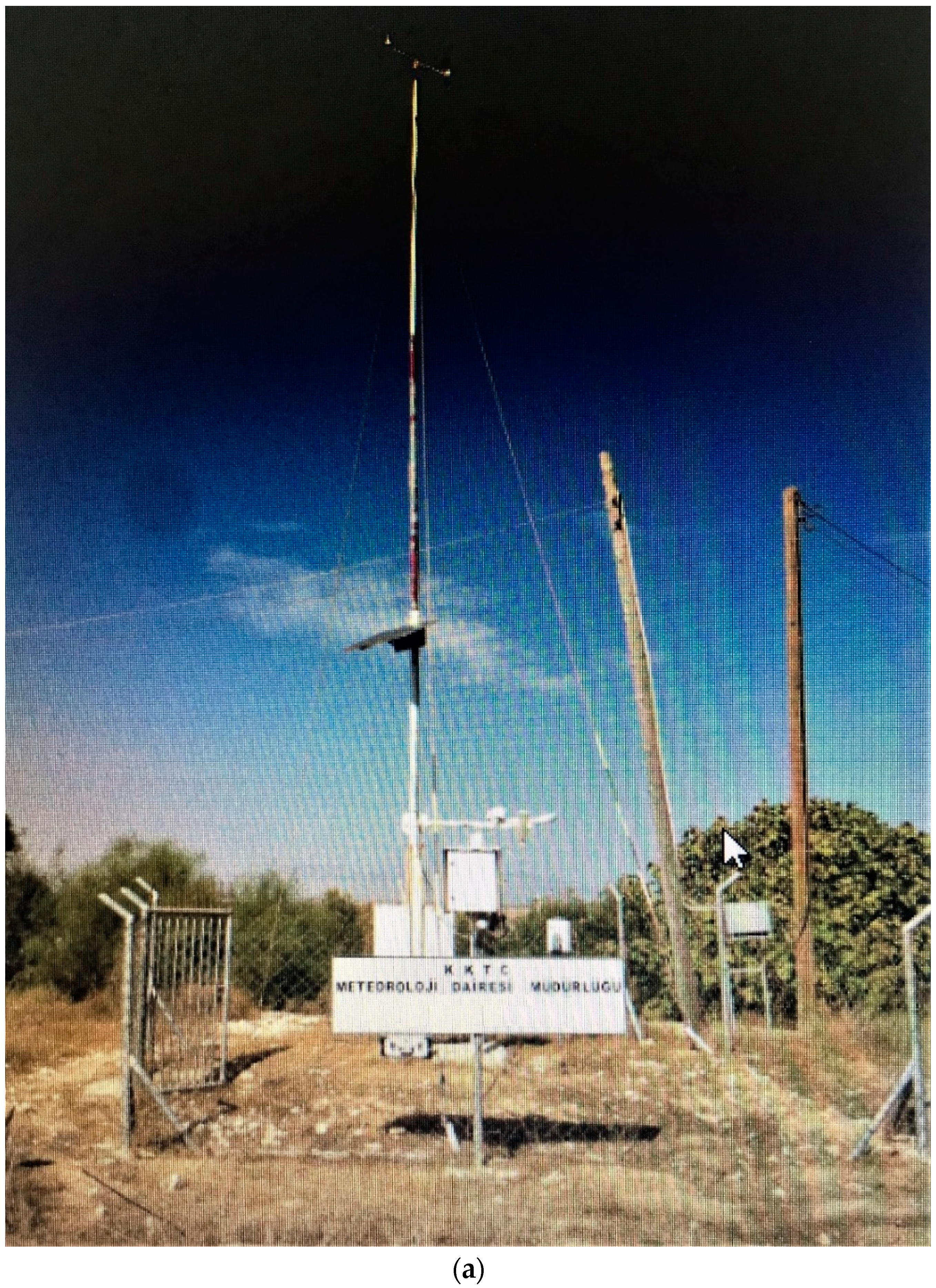
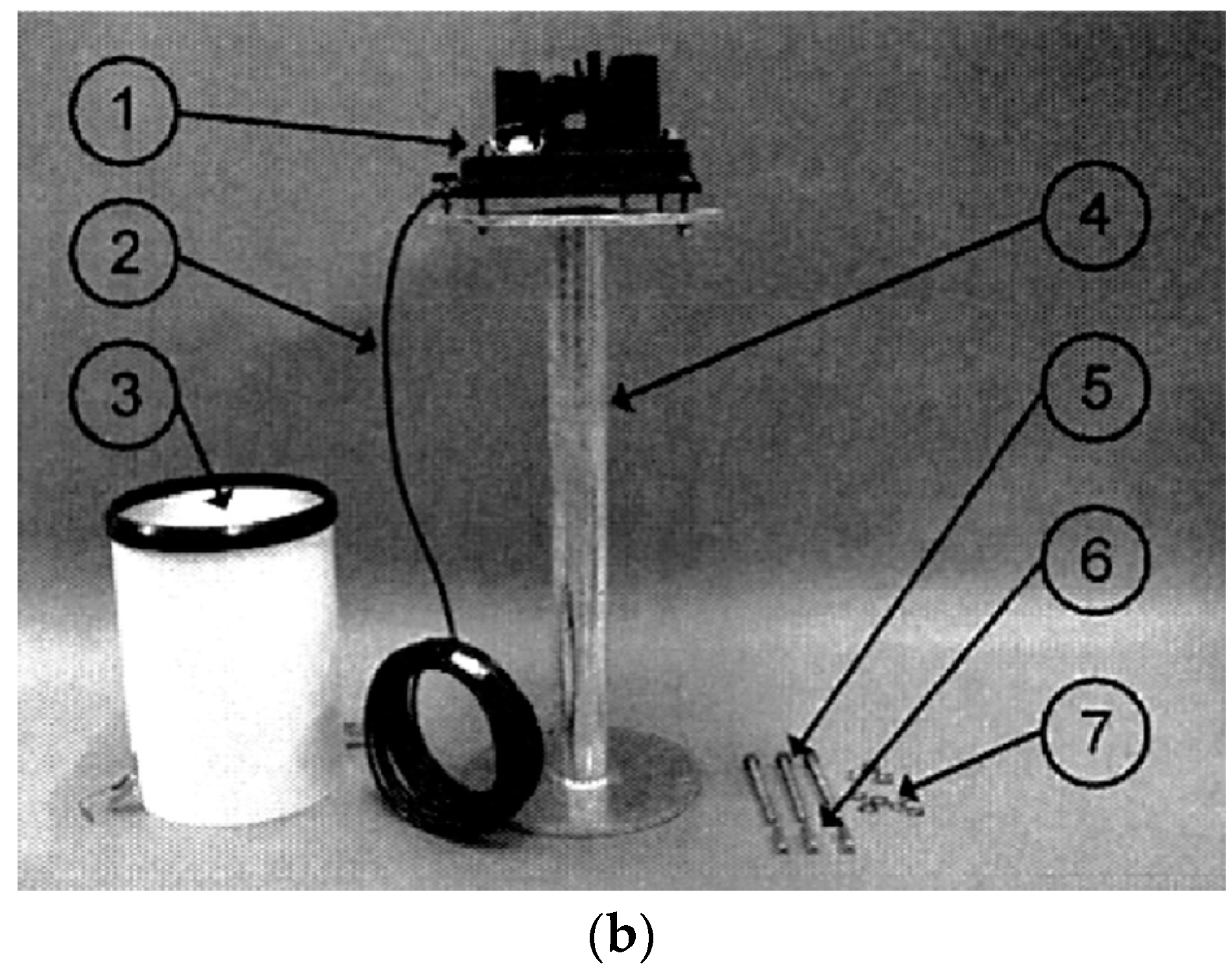
Figure 3.
Correlogram of precipitation time series for (a) Ercan station; (b) Lefkoşa station. UL = Upper Limit; LL = Lower Limit.
Figure 3.
Correlogram of precipitation time series for (a) Ercan station; (b) Lefkoşa station. UL = Upper Limit; LL = Lower Limit.

Figure 4.
Conceptual model of the ensemble system in scenario 1.
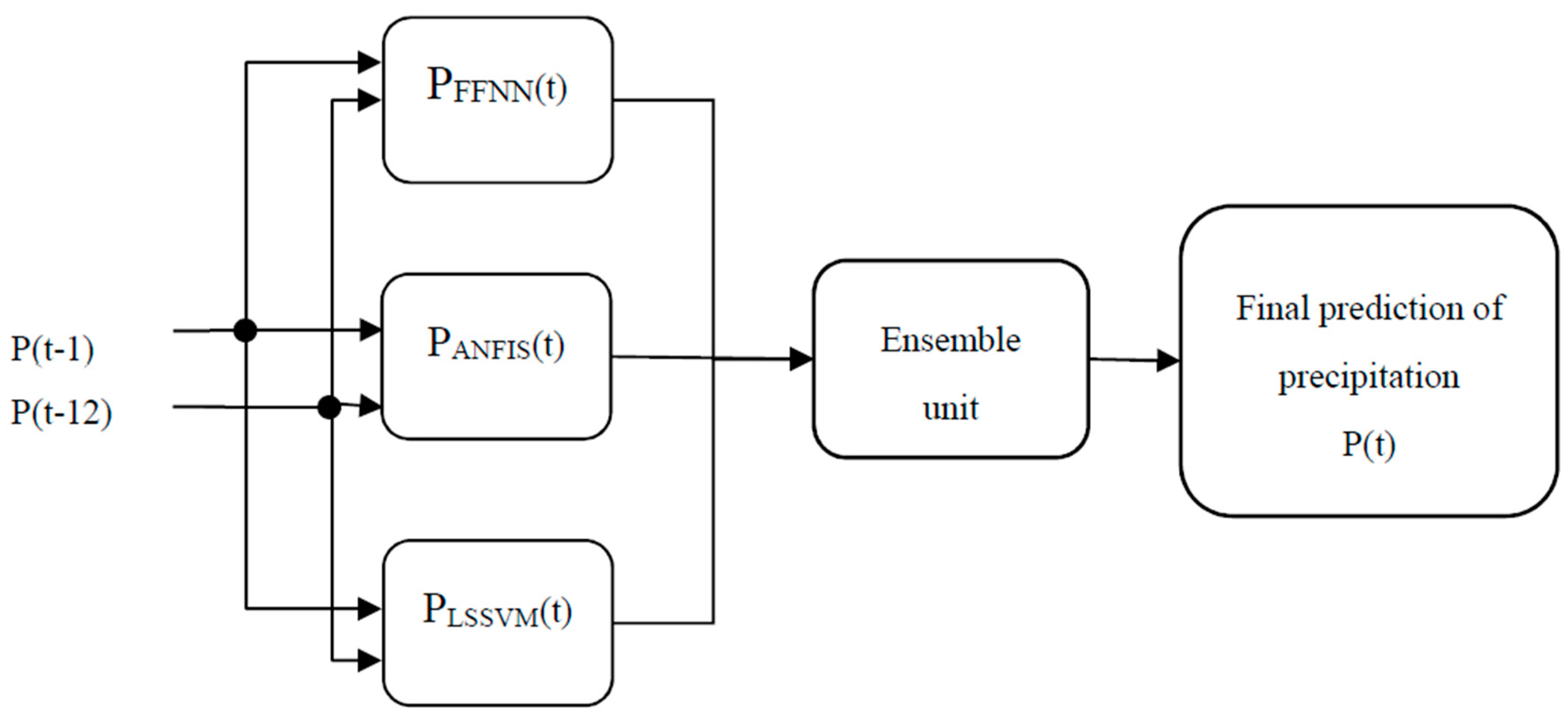
Figure 5.
Structure of a three-layer feed forward neural network (FFNN).
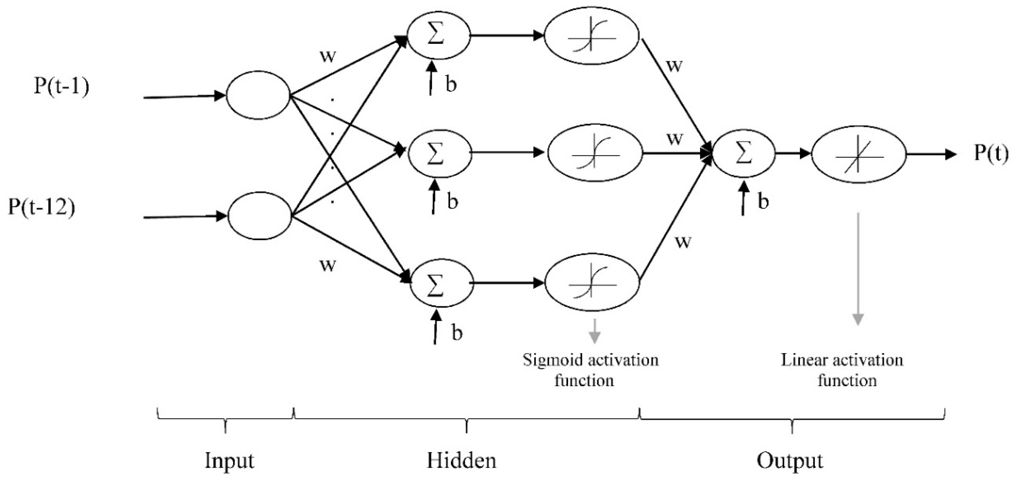
Figure 6.
Adaptive neural fuzzy inference system (ANFIS) structure.
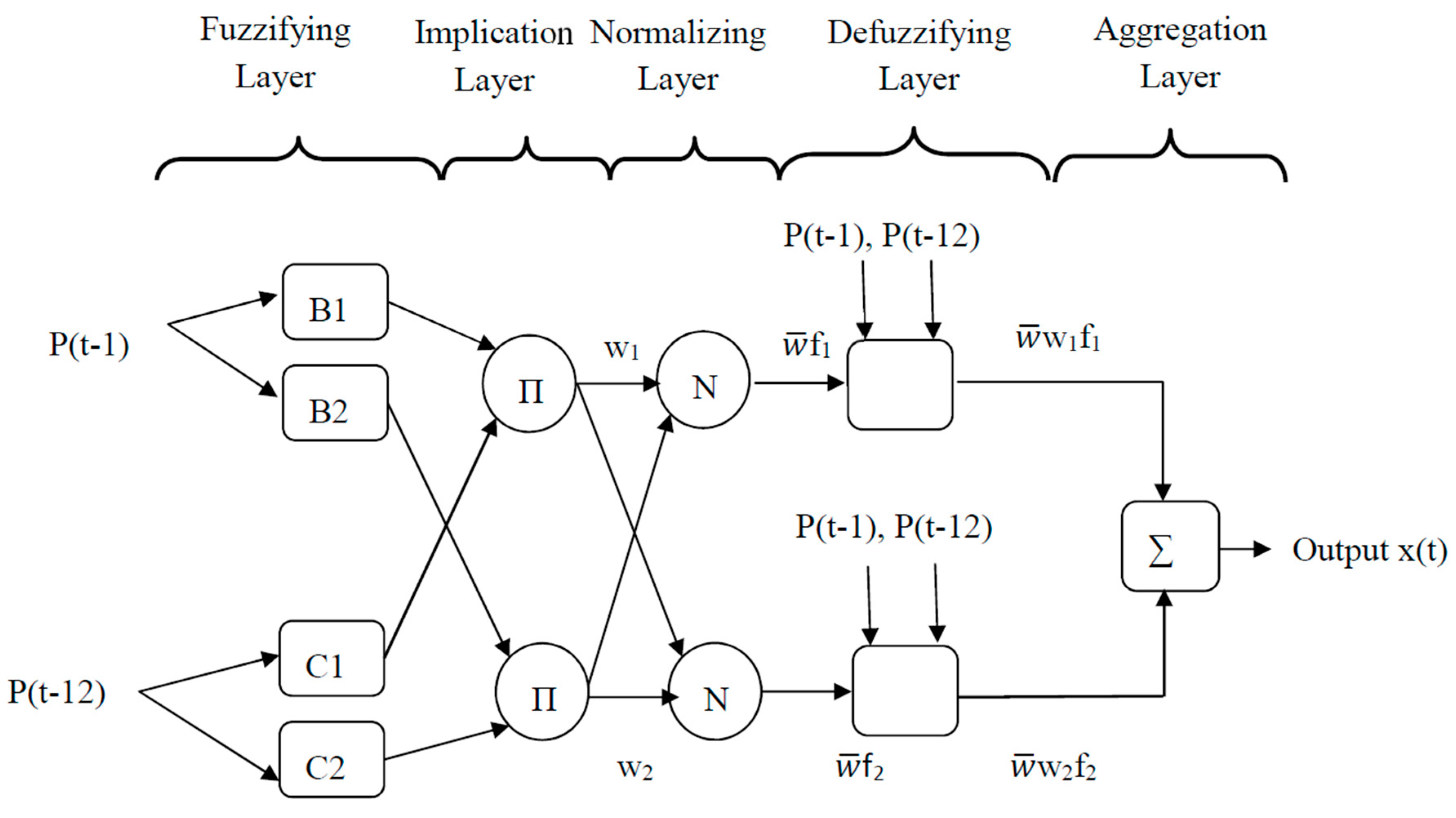
Figure 7.
Structure of least square support vector machine (LSSVM).
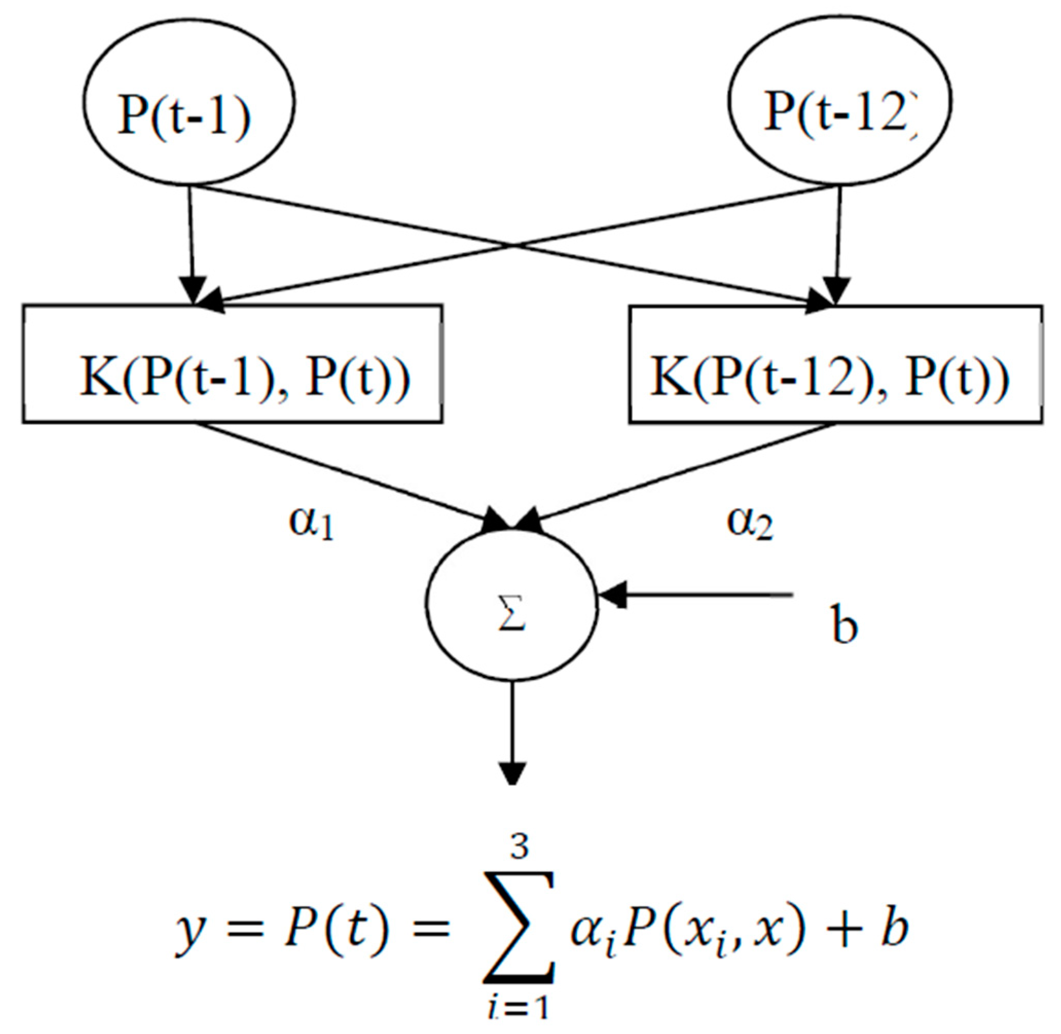
Figure 8.
Schematic of the proposed neural ensemble method. ANN: artificial neural networks.
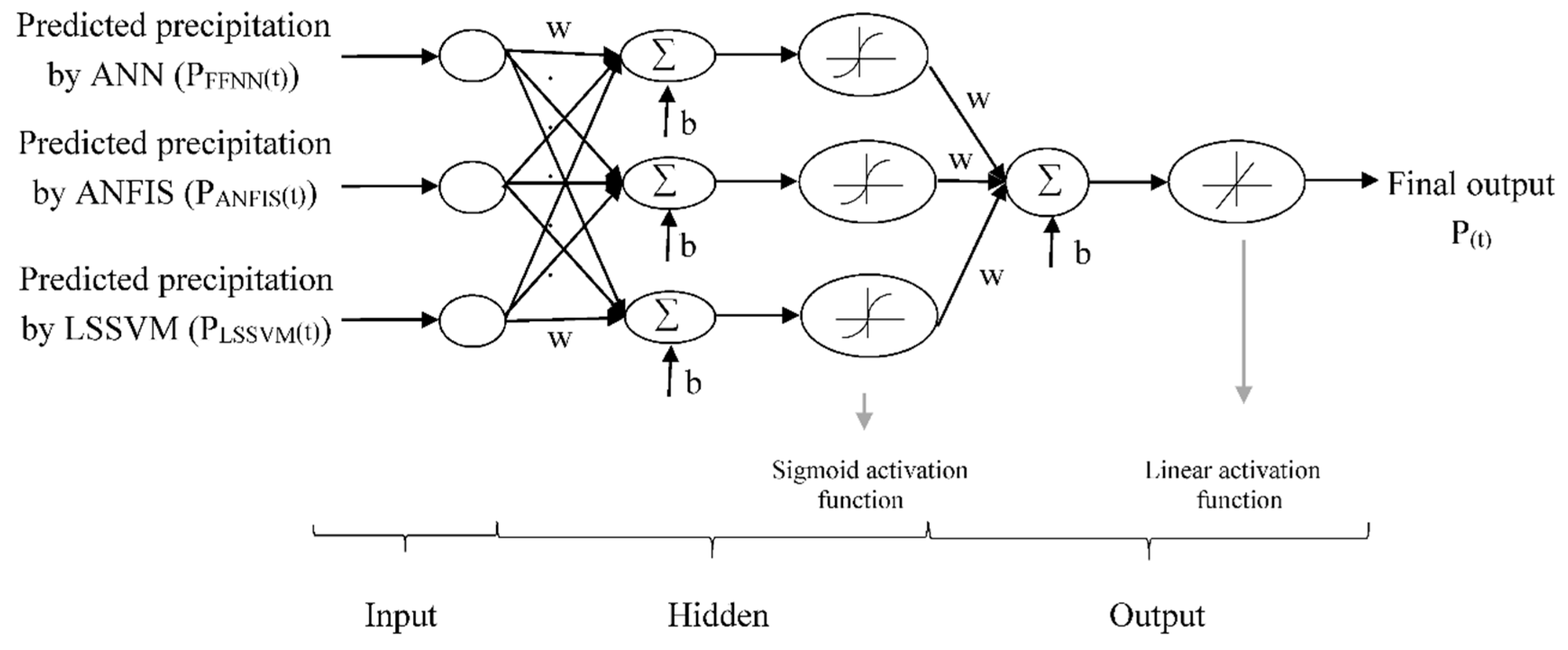
Figure 9.
(a) Observed versus computed precipitation time series by FFNN, ANFIS and LSSVM models. Scatter plots for verification step for (b) FFNN; (c) ANFIS; (d) LSSVM models via scenario 1 for Ercan station.
Figure 9.
(a) Observed versus computed precipitation time series by FFNN, ANFIS and LSSVM models. Scatter plots for verification step for (b) FFNN; (c) ANFIS; (d) LSSVM models via scenario 1 for Ercan station.
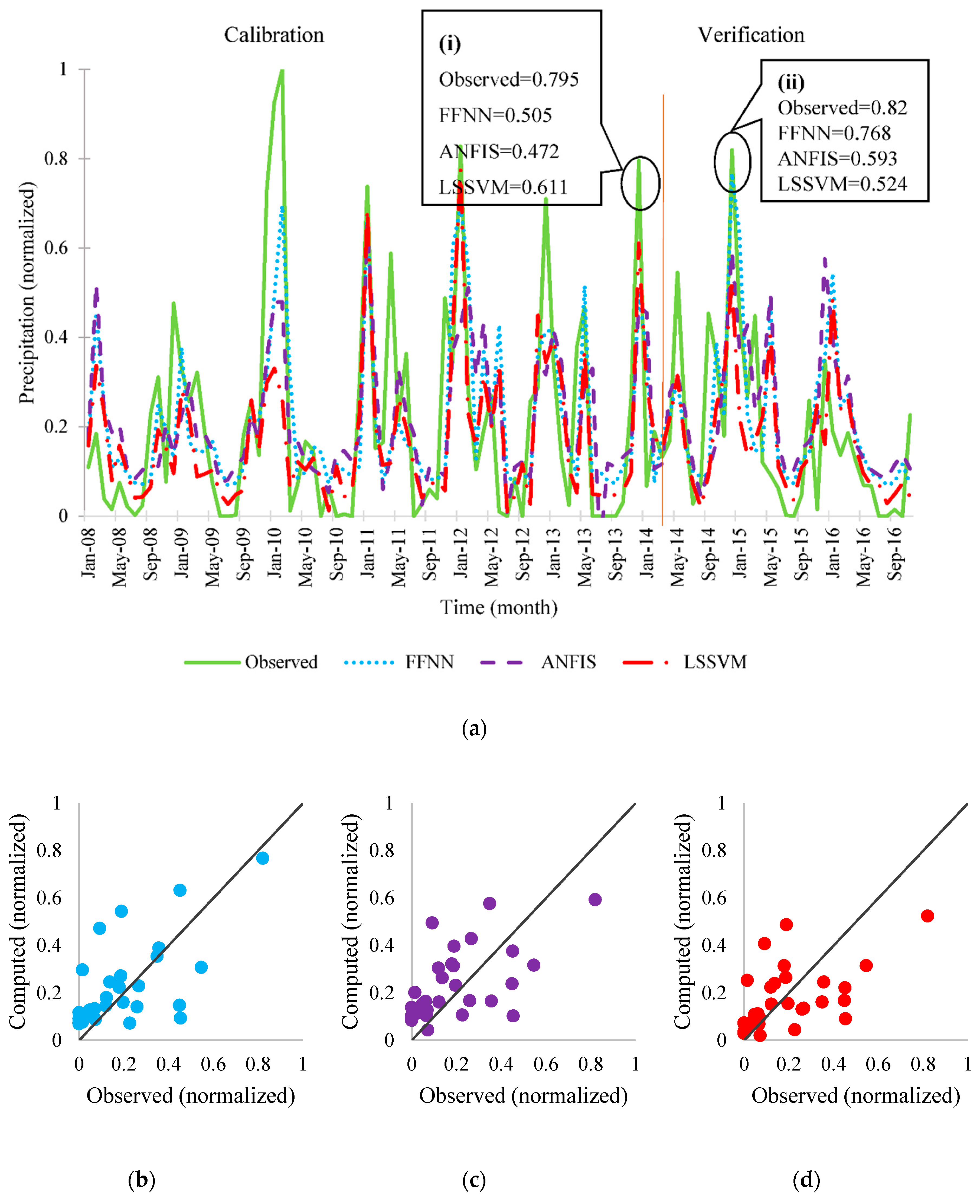
Figure 10.
(a) Observed versus computed precipitation time series by FFNN, ANFIS and LSSVM models. Scatter plots for verification step for (b) FFNN; (c) ANFIS; (d) LSSVM models via scenario 1 for Girne station.
Figure 10.
(a) Observed versus computed precipitation time series by FFNN, ANFIS and LSSVM models. Scatter plots for verification step for (b) FFNN; (c) ANFIS; (d) LSSVM models via scenario 1 for Girne station.
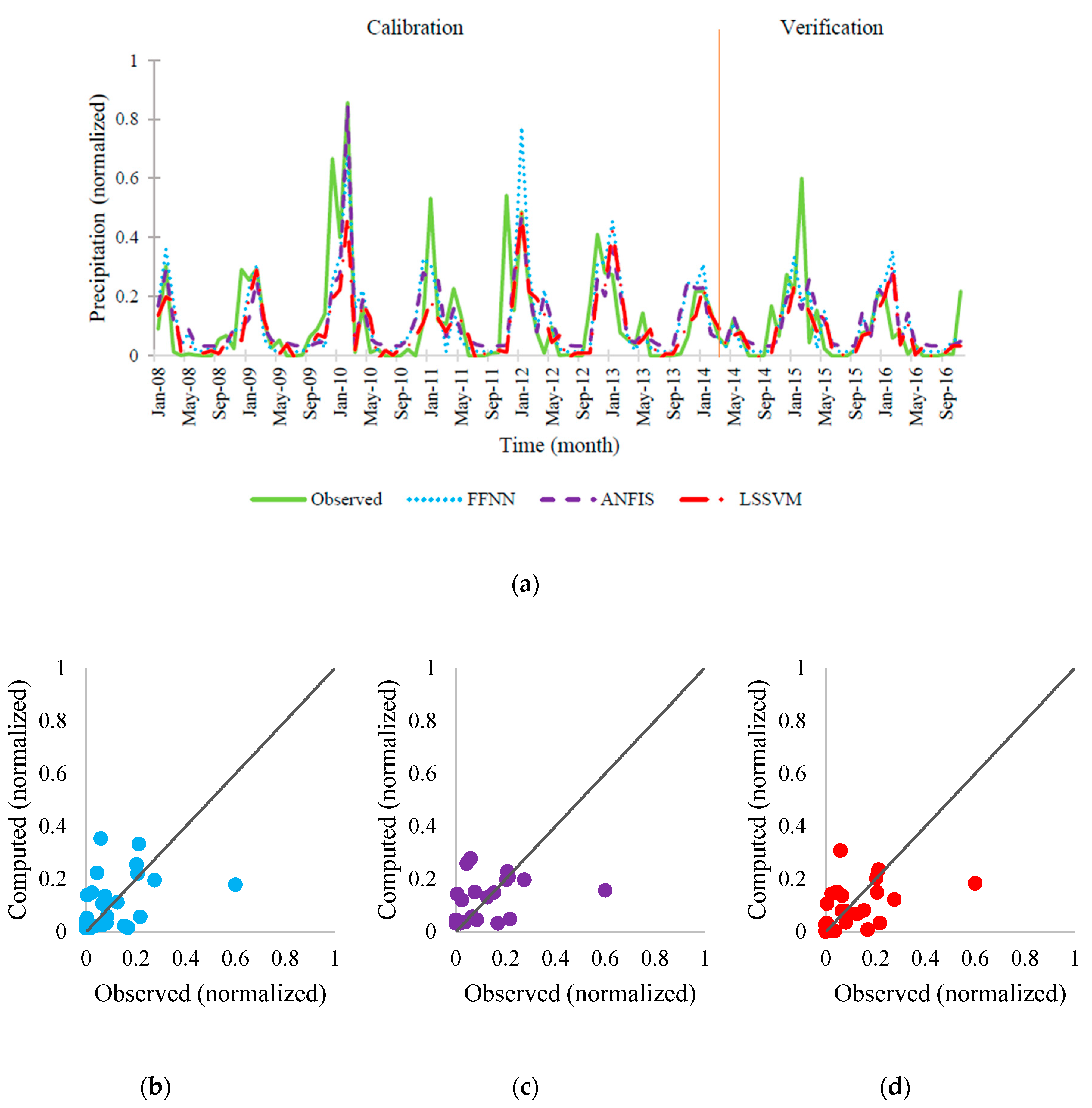
Figure 11.
(a) Observed versus computed precipitation time series by FFNN, ANFIS and LSSVM models. Scatter plots for verification step for (b) FFNN; (c) ANFIS; (d) LSSVM models via scenario 2 for Girne station.
Figure 11.
(a) Observed versus computed precipitation time series by FFNN, ANFIS and LSSVM models. Scatter plots for verification step for (b) FFNN; (c) ANFIS; (d) LSSVM models via scenario 2 for Girne station.

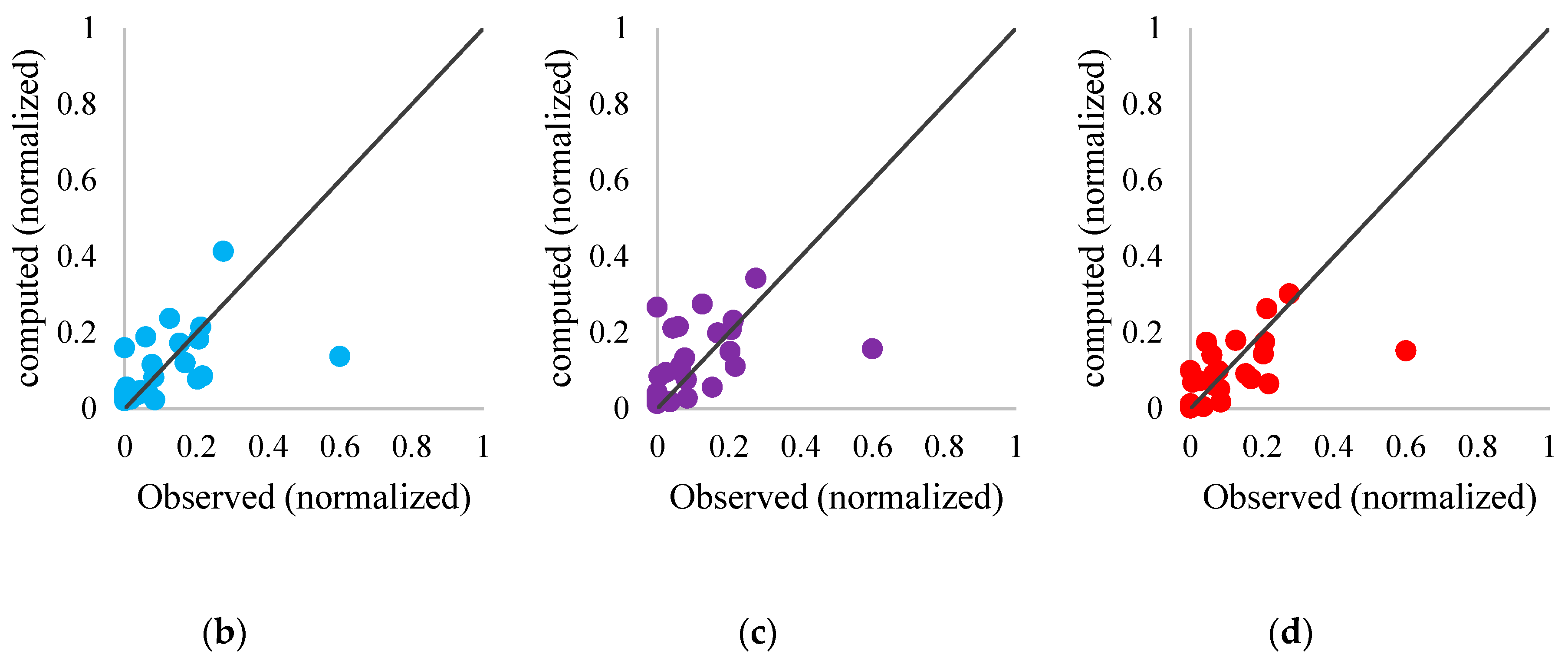
Figure 12.
(a) Results of precipitation prediction using simple, weighted and neural averaging methods and observed precipitation; (b) Scatter plots for verification step using neural ensemble method based on scenario 2 for Girne station.
Figure 12.
(a) Results of precipitation prediction using simple, weighted and neural averaging methods and observed precipitation; (b) Scatter plots for verification step using neural ensemble method based on scenario 2 for Girne station.


Figure 13.
Scatter plot for verification step using FFNN and neural ensemble method based on scenario 2 for Girne station.
Figure 13.
Scatter plot for verification step using FFNN and neural ensemble method based on scenario 2 for Girne station.


Table 1.
Specifications of rain gauges.
| Property | Description/Value |
|---|---|
| Sensor/Transducer type | Tipping bucket/Reed switch |
| Precipitation type | Liquid |
| Accuracy | ±2% |
| Sensitivity | 0.2 mm |
| Closure time | <100 ms (for 0.2 mm of rain) |
| Capacity | Unlimited |
| Funnel diameter | 225 mm |
| Standard | 400 cm2 |
| With expander unit | 1000 cm2 |
| Max. current rating | 500 mA |
| Breakdown voltage | 400 VDC |
| Capacity open contacts | 0.2 pF |
| Life (operations) | 108 closures |
| Material | Non-corrosive aluminum alloy LM25 |
| Dimensions | 390 (h) × 300 (Ø) mm |
| Weight | 2.5 kg |
| Temperature range (operating) | 0–+85 °C |
Table 2.
The characteristics of stations and statistics of the precipitation data.
| Station | Altitude (m) | Longitude | Latitude | Max Precipitation (mm/month) | Mean Precipitation (mm/month) | Std. Deviation of Precipitation (mm/month) |
|---|---|---|---|---|---|---|
| Ercan | 123 m | 33°29′59.99″ E | 35°09′21.00″ N | 2130.0 | 25.2 | 29.1 |
| Gazimağusa | 1.8 m | 33°56′20.18″ E | 35°7′13.94″ N | 3141.0 | 27.9 | 38.1 |
| Geçitkale | 44 m | 33°23′15″ E | 34°49′30″ N | 2100.0 | 27 | 33.6 |
| Girne | 0 m | 33°19′2.24” E | 35°20′10.82″ N | 4260.0 | 38.4 | 58.5 |
| Güzelyurt | 65 m | 32°59′36.17″ E | 35°11′55.28″ N | 3021.0 | 23.7 | 30 |
| Lefkoşa | 220 m | 33°21′51.12″ E | 35°10′31.12″ N | 1986.0 | 22.8 | 27.6 |
| Yeni Erenköy | 22 m | 34°11′30″ E | 35°31′60″ N | 2280.0 | 33.3 | 43.8 |
Table 3.
The mutual information (MI) between the observed precipitation time series of statins.
| Station | Ercan | Gazimağusa | Geçitkale | Girne | Güzelyurt | Lefkoşa | Yeni Erenköy |
|---|---|---|---|---|---|---|---|
| Ercan | 1.468 | - | - | - | - | - | - |
| Gazimağusa | 0.993 | 1.269 | - | - | - | - | - |
| Geçitkale | 1.038 | 0.939 | 1.294 | - | - | - | - |
| Girne | 1.085 | 0.893 | 0.868 | 1.204 | - | - | - |
| Güzelyurt | 0.958 | 0.964 | 0.908 | 0.911 | 1.281 | - | - |
| Lefkoşa | 1.074 | 0.971 | 0.974 | 0.949 | 0.983 | 1.3265 | - |
| Yeni Erenköy | 0.992 | 0.941 | 0.925 | 0.876 | 0.947 | 0.9673 | 1.278 |
| Mean MI | 1.02 | 0.95 | 0.942 | 0.931 | 0.945 | 0.986 | 0.941 |
Table 4.
Results of monthly precipitation predictions by FFNN for both scenarios 1 and 2.
| Station | Scenario | Epoch | Network Structure a | DC | RMSE (Normalized) | ||
|---|---|---|---|---|---|---|---|
| Calibration | Verification | Calibration | Verification | ||||
| Ercan | 1 | 20 | (3.14.1) | 0.670 | 0.637 | 0.176 | 0.157 |
| Gazimağusa | 1 | 60 | (3.2.1) | 0.547 | 0.538 | 0.183 | 0.120 |
| 2 | 10 | (4.10.1) | 0.766 | 0.684 | 0.144 | 0.106 | |
| Geçitkale | 1 | 90 | (3.4.1) | 0.673 | 0.503 | 0.147 | 0.099 |
| 2 | 20 | (4.11.1) | 0.845 | 0.677 | 0.108 | 0.087 | |
| Girne | 1 | 30 | (3.16.1) | 0.729 | 0.511 | 0.119 | 0.169 |
| 2 | 10 | (4.12.1) | 0.800 | 0.728 | 0.101 | 0.135 | |
| Güzelyurt | 1 | 10 | (3.5.1) | 0.723 | 0.423 | 0.150 | 0.145 |
| 2 | 10 | (4.18.1) | 0.854 | 0.664 | 0.114 | 0.131 | |
| Lefkoşa | 1 | 20 | (3.17.1) | 0.585 | 0.545 | 0.172 | 0.138 |
| 2 | 10 | (4.3.1) | 0.768 | 0.621 | 0.142 | 0.124 | |
| Yeni Erenköy | 1 | 40 | (3.4.1) | 0.570 | 0.474 | 0.134 | 0.079 |
| 2 | 20 | (4.11.1) | 0.835 | 0.692 | 0.090 | 0.069 | |
a Only the results of the optimum models have been tabulated. In network structure (a.b.c) a,b,c respectively show the numbers of input, hidden, and output neurons.
Table 5.
Results of monthly precipitation predictions by ANFIS model both scenarios 1 and 2.
| Station | Scenario | Epoch | Network Structure a | DC | RMSE (Normalized) | ||
|---|---|---|---|---|---|---|---|
| Calibration | Verification | Calibration | Verification | ||||
| Ercan | 1 | 5 | trimf-2 | 0.591 | 0.582 | 0.195 | 0.162 |
| Gazimağusa | 1 | 35 | trimf-2 | 0.510 | 0.479 | 0.188 | 0.126 |
| 2 | 80 | pimf-2 | 0.823 | 0.633 | 0.104 | 0.117 | |
| Geçitkale | 1 | 10 | trimf-3 | 0.728 | 0.483 | 0.127 | 0.102 |
| 2 | 5 | gauss2mf-2 | 0.840 | 0.630 | 0.107 | 0.099 | |
| Girne | 1 | 75 | trimf-2 | 0.716 | 0.439 | 0.111 | 0.180 |
| 2 | 5 | trimf-2 | 0.876 | 0.678 | 0.075 | 0.158 | |
| Güzelyurt | 1 | 95 | trimf-2 | 0.700 | 0.418 | 0.128 | 0.148 |
| 2 | 5 | trimf-2 | 0.893 | 0.645 | 0.071 | 0.144 | |
| Lefkoşa | 1 | 100 | trimf-2 | 0.554 | 0.515 | 0.176 | 0.137 |
| 2 | 5 | trimf-2 | 0.869 | 0.609 | 0.092 | 0.135 | |
| Yeni Erenköy | 1 | 15 | gaussmf-2 | 0.617 | 0.447 | 0.127 | 0.082 |
| 2 | 10 | gaussmf-2 | 0.899 | 0.617 | 0.071 | 0.074 | |
a trimf: triangular-shaped MF; gaussmf: Gaussian curve MF; gauss2mf: two Gaussian combination MF; pimf: pi shaped MF.
Table 6.
Results of monthly rainfall predictions by LSSVM for both scenarios 1 and 2.
| Station | Scenario | Network Structure a | DC | RMSE (Normalized) | ||
|---|---|---|---|---|---|---|
| Calibration | Verification | Calibration | Verification | |||
| Ercan | 1 | (10,2,0.1) | 0.655 | 0.556 | 0.184 | 0.162 |
| Gazimağusa | 1 | (10,0.3,0.3333) | 0.550 | 0.497 | 0.185 | 0.123 |
| 2 | (10,0.3,0.3333) | 0.816 | 0.680 | 0.129 | 0.115 | |
| Geçitkale | 1 | (20,0.1,1) | 0.676 | 0.507 | 0.150 | 0.102 |
| 2 | (20,0.1,1) | 0.866 | 0.654 | 0.089 | 0.110 | |
| Girne | 1 | (50,0.01,0.3333) | 0.704 | 0.502 | 0.123 | 0.177 |
| 2 | (50,0.01,0.3333) | 0.876 | 0.701 | 0.085 | 0.148 | |
| Güzelyurt | 1 | (1,0.2,0.3333) | 0.727 | 0.415 | 0.156 | 0.143 |
| 2 | (1,0.2,0.3333) | 0.894 | 0.657 | 0.109 | 0.122 | |
| Lefkoşa | 1 | (60,0.2,0.5) | 0.582 | 0.530 | 0.173 | 0.142 |
| 2 | (60,0.2,0.5) | 0.769 | 0.588 | 0.098 | 0.139 | |
| Yeni Erenköy | 1 | (60,0.01,0.3333) | 0.619 | 0.473 | 0.132 | 0.084 |
| 2 | (60,0.01,0.3333) | 0.852 | 0.670 | 0.086 | 0.068 | |
a Structure shows (λ, ε, c).
Table 7.
Results of ensembles using linear weighted and non-linear averaging methods for scenario 1.
Table 7.
Results of ensembles using linear weighted and non-linear averaging methods for scenario 1.
| Station | Ensemble Method | Model Structure a | Determination Coefficient (DC) | Root Mean Square Error (RMSE) (Normalized) | ||
|---|---|---|---|---|---|---|
| Calibration | Verification | Calibration | Verification | |||
| Ercan | Simple linear averaging | - | 0.678 | 0.643 | 0.177 | 0.149 |
| Weighted averaging | 0.357-0.331-0.312 | 0.680 | 0.644 | 0.177 | 0.149 | |
| Non-linear averaging | (3,16,1) | 0.786 | 0.677 | 0.148 | 0.146 | |
| Gazimağusa | Simple linear averaging | - | 0.560 | 0.520 | 0.182 | 0.121 |
| Weighted averaging | 0.347-0.320-0.333 | 0.559 | 0.521 | 0.182 | 0.121 | |
| Non-linear averaging | (3,3,1) | 0.702 | 0.540 | 0.155 | 0.126 | |
| Geçitkale | Simple linear averaging | - | 0.7431 | 0.650 | 0.134 | 0.094 |
| Weighted averaging | 0.337-0.323-0.340 | 0.741 | 0.651 | 0.135 | 0.094 | |
| Non-linear averaging | (3,12,1) | 0.765 | 0.670 | 0.128 | 0.092 | |
| Girne | Simple linear averaging | - | 0.753 | 0.516 | 0.111 | 0.173 |
| Weighted averaging | 0.352-0.302-0.346 | 0.750 | 0.522 | 0.112 | 0.173 | |
| Non-linear averaging | (3,11,1) | 0.825 | 0.678 | 0.095 | 0.157 | |
| Güzelyurt | Simple linear averaging | - | 0.779 | 0.432 | 0.139 | 0.143 |
| Weighted averaging | 0.337-0.333-0.330 | 0.776 | 0.433 | 0.140 | 0.143 | |
| Non-linear averaging | (3,4,1) | 0.774 | 0.447 | 0.137 | 0.143 | |
| Lefkoşa | Simple linear averaging | - | 0.594 | 0.561 | 0.171 | 0.138 |
| Weighted averaging | 0.343-0.324-0.333 | 0.592 | 0.564 | 0.171 | 0.138 | |
| Non-linear averaging | (3,2,1) | 0.706 | 0.585 | 0.150 | 0.138 | |
| Yeni Erenköy | Simple linear averaging | - | 0.628 | 0.489 | 0.128 | 0.081 |
| Weighted averaging | 0.340-0.321-0.339 | 0.623 | 0.489 | 0.129 | 0.080 | |
| Non-linear averaging | (3,13,1) | 0.690 | 0.491 | 0.118 | 0.079 | |
a Model structure in weighted averaging method shows applied weights respectively on FFNN, ANFIS and LSSVM outputs, whereas for neural averaging it shows numbers of input, hidden and output neurons, respectively.
Table 8.
Results of ensembles using linear, weighted and non-linear averaging methods for scenario 2.
Table 8.
Results of ensembles using linear, weighted and non-linear averaging methods for scenario 2.
| Station | Ensemble Method | Model Structure a | DC | RMSE (Normalized) | ||
|---|---|---|---|---|---|---|
| Calibration | Verification | Calibration | Verification | |||
| Gazimağusa | Simple linear averaging | - | 0.851 | 0.699 | 0.116 | 0.107 |
| Weighted averaging | 0.336-0.320-0.344 | 0.847 | 0.699 | 0.118 | 0.107 | |
| Non-linear averaging | (3,20,1) | 0.900 | 0.722 | 0.095 | 0.102 | |
| Geçitkale | Simple linear averaging | - | 0.880 | 0.681 | 0.096 | 0.096 |
| Weighted averaging | 0.345-0.321-0.334 | 0.873 | 0.691 | 0.099 | 0.093 | |
| Non-linear averaging | (3,5,1) | 0.883 | 0.727 | 0.100 | 0.086 | |
| Girne | Simple linear averaging | - | 0.889 | 0.734 | 0.079 | 0.144 |
| Weighted averaging | 0.345-0.322-0.333 | 0.884 | 0.744 | 0.080 | 0.142 | |
| Non-linear averaging | (3,16,1) | 0.947 | 0.813 | 0.090 | 0.122 | |
| Güzelyurt | Simple linear averaging | - | 0.923 | 0.686 | 0.089 | 0.124 |
| Weighted averaging | 0.338-0.328-0.334 | 0.913 | 0.681 | 0.096 | 0.123 | |
| Non-linear averaging | (3,18,1) | 0.885 | 0.668 | 0.106 | 0.121 | |
| Lefkoşa | Simple linear averaging | - | 0.895 | 0.627 | 0.101 | 0.127 |
| Weighted averaging | 0.342-0.335-0.323 | 0.884 | 0.633 | 0.107 | 0.125 | |
| Non-linear averaging | (3,17,1) | 0.953 | 0.691 | 0.064 | 0.123 | |
| Yeni Erenköy | Simple linear averaging | - | 0.884 | 0.690 | 0.077 | 0.067 |
| Weighted averaging | 0.350-0.312-0.338 | 0.880 | 0.690 | 0.078 | 0.067 | |
| Non-linear averaging | (3,19,1) | 0.929 | 0.787 | 0.060 | 0.059 | |
a Model structure in weighted averaging method shows applied weights respectively on FFNN, ANFIS and LSSVM outputs, whereas for neural averaging it shows numbers of input, hidden and output neurons, respectively.
Table 9.
Skill scores of ensembles using linear, weighted and non-linear averaging methods for scenarios 1 and 2.
Table 9.
Skill scores of ensembles using linear, weighted and non-linear averaging methods for scenarios 1 and 2.
| Station | Scenario | Reference Model | Skill Score % | |||||
|---|---|---|---|---|---|---|---|---|
| Simple Linear Averaging | Weighted Averaging | Non-Linear Averaging | ||||||
| Calibration | Verification | Calibration | Verification | Calibration | Verification | |||
| Ercan | FFNN | 2.42 | 1.65 | 3.03 | 1.93 | 35.152 | 11.02 | |
| 1 | ANFIS | 21.27 | 14.59 | 21.76 | 14.83 | 47.68 | 22.73 | |
| LSSVM | 6.67 | 19.59 | 7.25 | 19.82 | 37.97 | 27.25 | ||
| Gazimağusa | 1 | FFNN | 2.87 | −3.90 | 2.65 | −3.68 | 34.22 | 0.43 |
| ANFIS | 10.20 | 7.87 | 10.00 | 8.06 | 39.18 | 11.71 | ||
| LSSVM | 2.22 | 4.57 | 2.00 | 4.77 | 33.78 | 8.55 | ||
| 2 | FFNN | 36.32 | 4.75 | 34.62 | 4.75 | 57.26 | 12.03 | |
| ANFIS | 15.82 | 17.98 | 13.56 | 17.98 | 43.50 | 24.25 | ||
| LSSVM | 19.02 | 5.94 | 16.85 | 5.94 | 45.65 | 13.13 | ||
| Geçitkale | 1 | FFNN | 21.44 | 29.58 | 20.80 | 29.78 | 28.13 | 33.60 |
| ANFIS | 5.55 | 32.30 | 4.78 | 32.50 | 13.60 | 36.17 | ||
| LSSVM | 20.71 | 29.01 | 20.06 | 29.21 | 27.47 | 33.06 | ||
| 2 | FFNN | 22.58 | 1.24 | 18.06 | 4.33 | 24.52 | 15.48 | |
| ANFIS | 25.00 | 13.78 | 20.63 | 16.49 | 26.88 | 26.22 | ||
| LSSVM | 10.45 | 7.80 | 5.22 | 10.69 | 12.69 | 21.10 | ||
| Girne | 1 | FFNN | 8.86 | 1.02 | 7.75 | 2.25 | 35.42 | 34.15 |
| ANFIS | 13.03 | 13.73 | 11.97 | 14.80 | 38.38 | 42.60 | ||
| LSSVM | 16.55 | 2.81 | 15.54 | 4.02 | 40.88 | 35.34 | ||
| 2 | FFNN | 44.50 | 2.21 | 42.00 | 5.88 | 73.50 | 31.25 | |
| ANFIS | 10.48 | 17.39 | 6.45 | 20.50 | 57.26 | 41.93 | ||
| LSSVM | 10.48 | 11.04 | 6.45 | 14.38 | 57.26 | 37.46 | ||
| Güzelyurt | 1 | FFNN | 20.22 | 1.56 | 19.13 | 1.73 | 18.41 | 4.16 |
| ANFIS | 26.33 | 2.41 | 25.33 | 2.58 | 24.67 | 4.98 | ||
| LSSVM | 19.05 | 2.91 | 17.95 | 3.08 | 17.22 | 5.47 | ||
| 2 | FFNN | 47.26 | 6.55 | 40.41 | 5.06 | 21.23 | 1.19 | |
| ANFIS | 28.04 | 11.55 | 18.69 | 10.14 | −7.48 | 6.48 | ||
| LSSVM | 27.36 | 8.45 | 17.92 | 7.00 | −8.49 | 3.21 | ||
| Lefkoşa | 1 | FFNN | 2.17 | 3.52 | 1.69 | 4.18 | 29.16 | 8.79 |
| ANFIS | 8.97 | 9.48 | 8.52 | 10.10 | 34.08 | 14.43 | ||
| LSSVM | 2.87 | 6.60 | 2.39 | 7.23 | 29.67 | 11.70 | ||
| 2 | FFNN | 54.74 | 1.58 | 50.00 | 3.17 | 79.74 | 18.47 | |
| ANFIS | 19.85 | 4.60 | 11.45 | 6.14 | 64.12 | 20.97 | ||
| LSSVM | 54.55 | 9.47 | 49.78 | 10.92 | 79.65 | 25.00 | ||
| Yeni Erenköy | 1 | FFNN | 13.49 | 2.85 | 12.33 | 2.85 | 27.91 | 3.23 |
| ANFIS | 2.87 | 7.59 | 1.57 | 7.59 | 19.06 | 7.96 | ||
| LSSVM | 2.36 | 3.04 | 1.05 | 3.04 | 18.64 | 3.42 | ||
| 2 | FFNN | 29.70 | −0.65 | 27.27 | −0.65 | 56.97 | 30.84 | |
| ANFIS | −14.85 | 19.06 | −18.81 | 19.06 | 29.70 | 44.39 | ||
| LSSVM | 21.62 | 6.06 | 18.92 | 6.06 | 52.03 | 35.45 | ||
© 2019 by the authors. Licensee MDPI, Basel, Switzerland. This article is an open access article distributed under the terms and conditions of the Creative Commons Attribution (CC BY) license (http://creativecommons.org/licenses/by/4.0/).
Share and Cite
MDPI and ACS Style
Nourani, V.; Uzelaltinbulat, S.; Sadikoglu, F.; Behfar, N. Artificial Intelligence Based Ensemble Modeling for Multi-Station Prediction of Precipitation. Atmosphere 2019, 10, 80. https://doi.org/10.3390/atmos10020080
AMA Style
Nourani V, Uzelaltinbulat S, Sadikoglu F, Behfar N. Artificial Intelligence Based Ensemble Modeling for Multi-Station Prediction of Precipitation. Atmosphere. 2019; 10(2):80. https://doi.org/10.3390/atmos10020080
Chicago/Turabian StyleNourani, Vahid, Selin Uzelaltinbulat, Fahreddin Sadikoglu, and Nazanin Behfar. 2019. "Artificial Intelligence Based Ensemble Modeling for Multi-Station Prediction of Precipitation" Atmosphere 10, no. 2: 80. https://doi.org/10.3390/atmos10020080
Note that from the first issue of 2016, this journal uses article numbers instead of page numbers. See further details here.