Simulating the Effects of Urban Parameterizations on the Passage of a Cold Front During a Pollution Episode in Megacity Shanghai

Abstract

Urbanization significantly influences meteorological conditions and air quality. Statistically, air pollution in the megacity of Shanghai usually occurs with cold weather fronts. An air pollution episode during a cold front was simulated using weather research and forecasting and the Community Multi-scale Air Quality model system. In this study, we used two urban schemes, a simple bulk scheme (denoted BULK) and the single-layer urban canopy model (SLUCM), to check the effects of urban parameterization. Our results showed that SLUCM better predicted the arrival time and cooling process of the cold front and more realistically simulated the moving process of the cold front. The improvement in the temperature and relative humidity simulation achieved using SLUCM was more effective under higher urbanization levels, whereas the wind speed simulation was better in rural areas. The simulated concentrations at sites with high urbanization were obviously improved by urban parameterization. The barrier role of the urban canopy during a cold front was better represented and was shown to cause a wider polluted area and higher pollutant concentration using SLUCM than with BULK. Overall, accurate meteorological simulations in the atmospheric boundary layer using SLUCM are expected to provide good prediction of urban air quality.

1. Introduction

Shanghai is located in the eastern section of the Yangtze River Delta, which is one of the three largest city-cluster areas in China, with a population of 20 million. Shanghai City has experienced rapid economic development and urban expansion. Since the 1980s and according to the national new urbanization report in 2015, Shanghai’s urbanization rate ranked first, at 87.6% in 2015 [1,2]. Shanghai has experienced a significant change in population and land use and land cover change, which has resulted in buildings displacing cultivated land [3]. Land use types and building density have dramatically changed in Shanghai since the 1980s. Both observations and simulations proved that urban surface change affects the meteorological conditions [4,5]. Urbanization converts the city surface to urban covers including tall buildings, thereby increasing the roughness of the surface over the urban area. The friction and drag of the buildings decrease the near-surface wind speed in the urban area. This aerodynamic effect has been observed in many cities [6,7]. The influence of urbanization on meteorological fields has been observed in the Yangtze River Delta [8]. Zhang et al. [9] documented that urbanization may cause a wind speed loss of more than 50% in the Yangtze River Delta over urbanized areas, and that this wind speed decrease may not only occur over urban areas but also on a regional scale.

Applying an urban parameterization scheme in meteorological models is a key requirement to accurately simulate the atmospheric boundary layer (ABL) [10,11,12]. Kusaka et al. [13] used the weather research and forecasting (WRF) model coupled with a single-layer canopy scheme to simulate the Tokyo heat island status. Teddy and Pullen [14] performed a 23-day temperature analysis using the WRF-urban canopy model (UCM) in the New York region. Zhang et al. [15] performed a heat island analysis using the WRF-UCM in the Suzhou area in China. Miao et al. [16] simulated the influence of the morphological characteristics of buildings on the urban boundary layer structure of Beijing using an urban boundary layer model. These efforts have shown that a mesoscale model with a canopy module has some advantages for simulating weather and fluxes in urban areas, and particularly the ability to better simulate the characteristics of an urban heat island. Although these studies identified the meteorological mechanisms related to urban schemes, the advantages and disadvantages of the urban schemes have still not been clearly identified. Additionally, the performance of urban schemes over megalopolises such as Shanghai is still uncertain.

Air quality is simultaneously affected by meteorological conditions and emission sources. The effects of meteorological conditions are known to closely interact with chemical compositions, chemical reaction processes, and physical-optical characteristics of air pollutants [17,18,19,20,21,22,23]. Emissions from the same polluter could cause the concentration of air pollutant to differ by dozens or even a hundred times in different weather conditions. Therefore, meteorological field simulation limits the precision of the air quality simulation. The use of wind, temperature, and ABL height (ABLH) is necessary to understand the transport and diffusion of air pollutants within the boundary layer. Fan et al. [24] simulated the structure and characteristics of the ABL over the Pearl River Delta and noted that ABL characteristics are important for identifying air pollution problems. Therefore, accurately simulating the ABL characteristics will help to better predict the urban air quality in Shanghai.

Cold front system are important synoptic systems involved in heavy air pollution in China. These systems produce a difference in the wind ahead of and behind a cold front, and changes in ABL height (ABLH) and vertical convection, which have significant impacts on regional accumulation and transportation of air pollutants [25]. Shahgedanova et al. [26] determined that the passage of a cold front causes high concentrations of pollutants in areas where the elevated sources were determined by analyzing the NO₂ concentration of multiple land use types and pollutant sources. Cannichael et al. [27] simulated the impact of a low-pressure system on the transfer process of ozone in spring time in East Asia and showed that cold front processes greatly influence the spatial distribution of ozone. Studies are lacking on the impact of cold front processes on air pollution focusing on China, especially for the megacity of Shanghai. Wang et al. [28] researched the influence of cold fronts on the air quality of Lanzhou by combining historical synoptic maps with data from observation sites. Cheng et al. [25] used the Community Multiscale Air Quality (CMAQ) and HYbrid Single-Particle Lagrangian Integrated Trajectory (HYSPLIT) models to simulate the air pollution processes of a typical strong cold front moving across Northeastern China.

We aimed to evaluate the ability of different urban schemes to simulate the characteristics of the ABL in the Shanghai metropolitan area. Section 2 describes the model settings. The observational data and synoptic situations are presented in Section 3. Comparisons of the measured and simulated data are presented in Section 4. Finally, the conclusions are provided in Section 5. All the time used in this study was Beijing time.

2. Model Simulation and Scheme Settings

The WRF mesoscale model was employed in this study. The WRF model consists of fully compressible nonhydrostatic equations on a staggered Arakawa C grid. Its vertical coordinate is a terrain-following hydrostatic pressure coordinate [29]. A three-dimensional (3D) Eulerian atmospheric chemistry and transport model, CMAQ model version 4.6, was applied to simulate the concentrations of the major pollutants. Designed as a “one-atmosphere” model, CMAQ can simultaneously address the complex couplings among several air quality issues across spatial scales ranging from local to hemispheric [30,31]. The emission inventory of Shanghai was developed with a 1 × 1 km resolution by the Shanghai Environmental Monitoring Center (SEMC) [32], in which the emission in the Baoshan district was updated by Tan et al. [33]. For areas outside Shanghai, the emission inventory was combined with the Regional Emission Inventory in Asia with Transport Chemical evolution over Pacific (TRACE-P). Detailed emission information was provided by Tan et al. [33].

2.1. Urban Schemes

The initial urban parameterization scheme of the WRF model is a bulk scheme (denoted BULK) [34] that uses a roughness length of 0.8 m to represent the effects of urban surfaces, a surface albedo of 0.15 to represent the radiation trapped in the urban canyons, a volumetric heat capacity of 3.0 MJ m⁻³ K⁻¹, and a thermal conductivity of 3.24 W m⁻¹ K⁻¹ to represent large heat storage by the urban buildings and roads. This approach was employed in real-time forecasts by Liu et al. [35]. Therefore, detailed land use data may affect the results of the BULK scheme predictions of the ABL characteristics.

The single-layer urban canopy model (SLUCM) is another urban parameterization in WRF, developed by Kusaka et al. [36] and Kusaka and Kimura [37]. The urban geometry is represented through infinitely long street canyons, and three different urban surfaces (roofs, walls, and roads) are recognized. Shadowing, reflections, and radiation trapping in the street canyon are considered, and an exponential wind profile is prescribed to deduce the wind speed in the canyon from the wind speed above the canyon, where the lowest grid point is located in the model. All the urban surfaces are categorized as roofs, walls, or roads. The sensible heat fluxes from the roofs, walls, and roads are introduced in the lowest atmospheric layer [38].

Two simulation schemes were carried out to drive WRF: (1) the BULK urban option and (2) the SLUCM urban option. Both of the simulations were verified by measurements at four observational sites (Figure 1).

2.2. Model Settings

In this study, the coarse domain covered the area between 20.4 and 41.3° N and 110.1 and 134.2° E, with a horizontal resolution of 27 × 27 km, whereas the inner most domain covered the area between 30.35 and 31.52° N and 120.52 and 122.07° E, and it had a horizontal resolution of 1 × 1 km. The boundary layer processes were resolved using 28 vertical sigma levels from the top to the surface level, in which 17 layers were less than 2 km. The primary physics options included the WRF single-moment 6-class microphysics scheme [39], Betts-Miller-Janjic cumulus parameterization, the Rapid Radiative Transfer Model (RRTM) long-wave radiation scheme, the Dudhia shortwave radiation scheme, the Eta similarity surface layer scheme, the Noah land surface model, and the Mellor-Yamada-Janjic boundary layer scheme. For the two inner domains (D03 and D04), convection was assumed to be well-resolved by the explicit microphysical parameterization scheme, and no cumulus parameterization scheme was used.

A summer pollution period, occurring during 1–8 July 2011, was simulated in this study. The primary focus was the ABL characteristics during a cold front period on 4–5 July 2011. The lateral and initial conditions for the WRF simulations in this study were obtained from a daily NCEP (National Centers for Environmental Prediction)/NCAR (national center for atmospheric research) reanalysis with 1 × 1 grid data. In the present study, the spin-up time was 12 h.

The land use required for the WRF Preprocessing System (WPS) in WRF was updated using the interpretation data from Shanghai aerial remote sensing images from 2007. According to the national land use classification (for trial use), the data were divided into 71 categories, and the file of geo-grid sub-module was modified by matching the 71 categories with U.S. Geological Survey (USGS)-33 [40]. Figure 2 shows the land use from 1980 USGS that was default packed in the WRF model and the updated land use for Shanghai City in 2007 used in this study. A comparison of the data showed that the urban area has considerable increased over the three decades from 1980 until 2007. In this simulation, three different urban classes (commercial or industrial (COI), high-intensity residential (HIR), and low-intensity residential (LIR) areas) and USGS 33-category land cover, derived from land use databases, were used (e.g., the National Land Cover Data for the United States (NLCD), developed by the USGS). Shanghai urban land was linked to three different urban classes by the impervious surface percentage: 20–49% defines LIR, 50–79% defines HIR, and 80–100% defines COI. Two different urban schemes were set in parallel simulations: (1) WRF with BULK and (2) WRF with SLUCM.

Table 1. Urban morphological parameters considered for the three urban classes: commercial or industrial (COI), high-intensity residential (HIR), and low-intensity residential (LIR).

Parameters	LIR	HIR	COI
Urban fraction (%)	0.75	0.85	0.95
Building height (m)	5	12.5	20
Road width (m)	10	15	20
Buildings 5 m tall (%)	55.3	1.0	0
Buildings 10 m tall (%)	24.7	14.0	2.0
Buildings 15 m tall (%)	12.4	42.3	4.6
Buildings 20 m tall (%)	7.6	27.7	5.4
Buildings 25 m tall (%)	0	10.2	18.8
Buildings 30 m tall (%)	0	4.8	8.0
Buildings 40 m tall (%)	0	0	18.7
Buildings 50 m tall (%)	0	0	15.5
Buildings 60 m tall (%)	0	0	27.0

lists the morphological parameters considered for the three urban classes in the SLUCM option.

Table 2. Thermal parameters used in the single-layer urban canopy model (SLUCM) for every urban class. λ is the thermal conductivity of the material, C is the specific heat of the material, T(int) is the initial temperature of the material and also the temperature of the deepest layer, ε is the emissivity of the surface, α is the albedo of the surface, and z₀ is the roughness length for momentum over the surface.

Surface	λ (W m−1 K−1)	C (× 106 J m−3 K−1)	T (°C)	ε	α	z0 (m)
Roof	3.24	3	20	0.9	0.2	0.01
Wall	3.24	3	20	0.9	0.2	-
Road	2.5	2.3	20	0.95	0.15	0.01

lists the thermal parameters for the SLUCM option.

3. Observational Data and Synoptic Situations in Shanghai

3.1. Statistical Synoptic Situations During Air-Pollution Days in 2011–2013

There are no uniform standards to judge pollution days from 2011 to 2013 since the Air Quality Index (AQI) was introduced in 2012. In this study, we defined days with a daily average concentration of PM_2.5 of 115 μg/m³ or more as pollution days and those with more than 150 μg/m³ as heavy pollution days. Based on these definitions, 83 pollution days were selected from the three years and classified into four kinds of weather pattern: equalizing pressure, saddle shaped field pattern, westerly in rear of high-pressure pattern, and cold front pattern. Detailed pollution days for different weather patterns are shown in

Table 3. Pollution days for different weather patterns.

Weather Pattern	Pollution Days	Heavy Pollution Days	Proportion (%) 1
Equalizing pressure	47	17	36.17
Saddle shaped field pattern	6	1	16.67
Westerly in rear of high-pressure pattern	18	5	27.78
Cold front	12	7	58.33

¹ heavy pollution days/pollution days × 100%.

. This shows that the probability of heavy pollution caused by cold front weather is higher than the other weather types. The cold front event that occurred in July 2011, a typical summer cold front that is difficult to predict in summer seasons, is important for simultaneously forecasting the meteorological field and pollution conditions.

3.2. Observational Data for the Simulated Case

We chose a pollution episode caused by a cold front to simulate the effects of urbanization on the meteorological conditions and concentrations of air pollutants. The test period occurred from Beijing time 8:00 a.m. on 1 July 2011 to 8:00 a.m. local time (UTC + 8) on 8 July 2011, including a pollution period. The four observational sites for meteorological conditions are shown in Figure 1b, including Baoshan (s1), Fudan (s2), Hongqiao (s3), and Pudong (s4). The observational data included hourly wind speed, wind direction, temperature, and relative humidity for the four sites. Site s1 was located in the Baoshan Meteorological Bureau, a national benchmark weather station in Northern Shanghai. At s1, radio soundings were performed to determine the mean velocity, wind direction, and temperature. Sounding balloons were launched two times per day (at 8:00 a.m. and 8:00 p.m. UTC + 8). Station s1 represents LIR areas. Station s2 was located on the roof of a 10-m building at Fudan University, a mixed-pollution urban site with residential areas and trafficked roads in Northeastern Shanghai. At s2, vertical measurements were conducted with light detection and ranging (LIDAR) technology. Station s2 represents HIR areas. Sites s3 and s4 were surface automatic observation stations. Station s3 is located at Hongqiao Airport, approximately in the middle of Shanghai. Station s4 was located at Pudong Airport, in Eastern Shanghai. Station s3 represents LIR areas, and s4 represents a rural environment. To effectively represent the spatiality of geography, we chose measurement sites that could widely cover the Shanghai domain. The temperature in other sites at Minghan, Chomgming, Nanhui, Qingpu, Chongming, Jinshan, and Fengxian were used to show the time evolution of the temperature field of the cold front. The ambient concentrations of air pollutants were obtained from monitoring sites named Baoshan, Xuhui, Minhang, Songjiang, Qingpu, Pudongbinhai, Pudong liuli, and Fengxian.

3.3. Weather and Pollution Situations for the Simulated Case

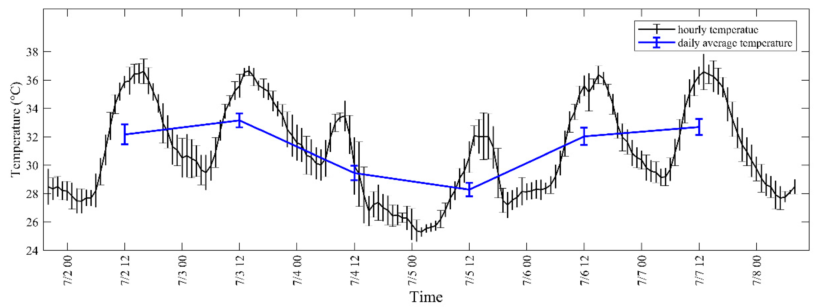
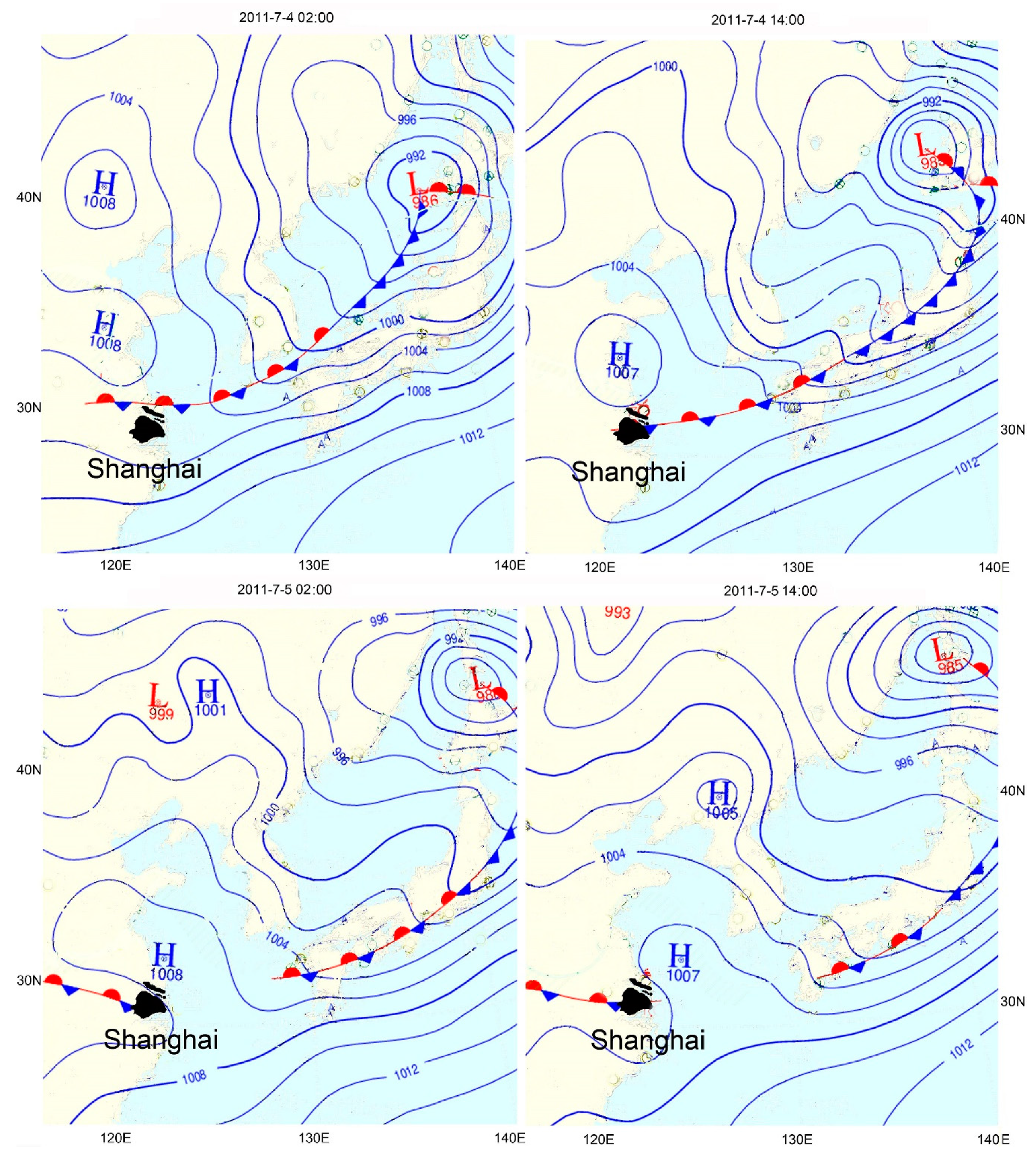
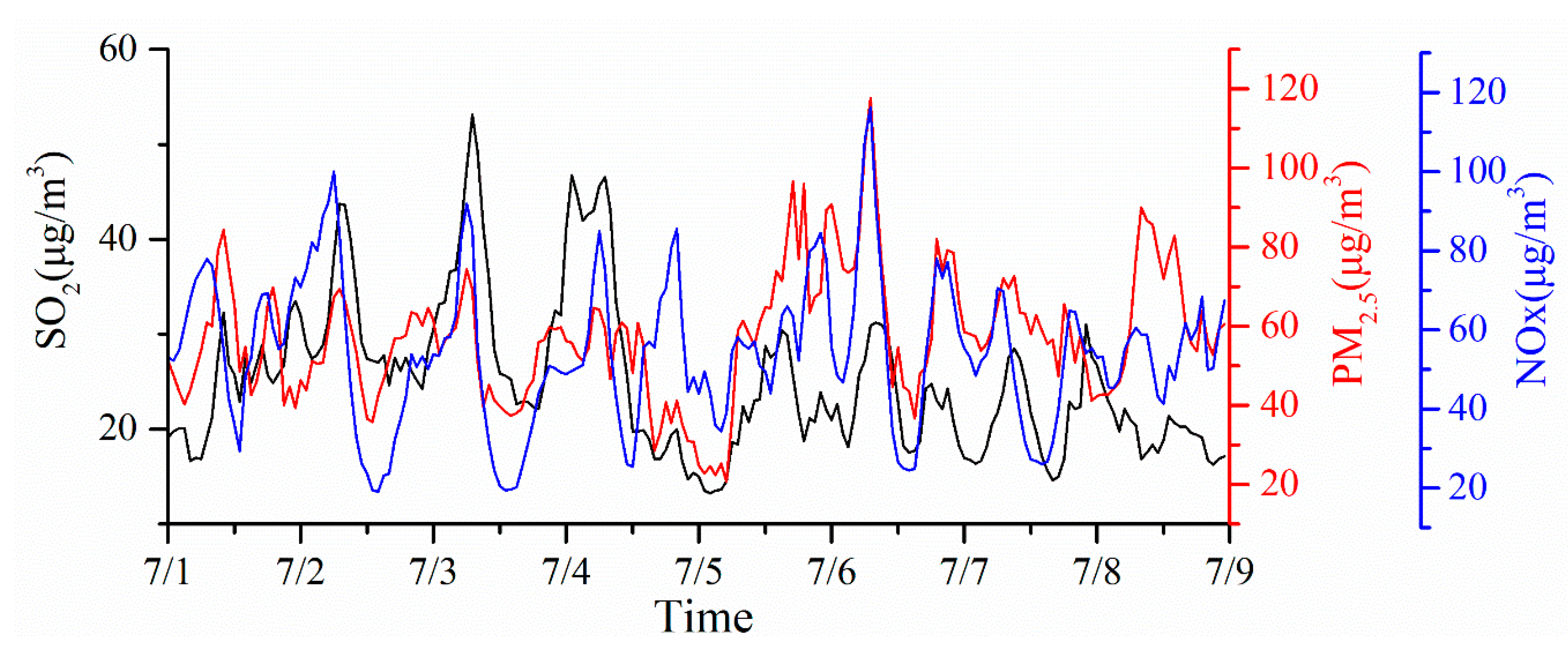
During the period of 1–8 July, the average temperature in Shanghai was approximately 31 °C, and the overall weather conditions were hot and rainy on some days (Figure 3). A cooling trend occurred on 4–5 July, caused by a cold front arriving in Shanghai, as shown in Figure 4. Severe convective weather appears to have promoted the spread of pollutants. Figure 5 shows the hourly concentrations of SO₂, NO_X, and PM_2.5 in Shanghai on 1–8 July. The normal diurnal variation of the three pollutants reached a peak at 8:00 a.m. and 8:00 p.m. each day. However, a special diurnal variation occurred on 4–5 July, caused by the cold front. This variation was characterized by an extremely low concentration during 2:00 p.m. July 4–12:00 a.m. July 5 followed by an extremely high concentration during 2:00–8:00 p.m. on July 5 (except for SO₂). In our study, during 10:00 a.m. to 3:00 p.m. on 4 July, the cold front was passing over Shanghai from the north of Shanghai, where the Baoshan site was located. The SO₂ concentration in Baoshan site had a particularly high concentration during 2:00–5:00 p.m. on 5 July, and a similar high concentration was not recorded at other sites. To test the ability of the WRF model to predict the characteristics of the ABL using different urban schemes, this period, 1–8 July, was used as a case study to analyze the passing of a cold front.

4. Comparison of the Measured Data and Simulated Results

4.1. Comparison of Statistical Parameters

To validate the WRF simulation results, the model results were compared with the available surface observations furnished by the meteorological stations in Domain 4. Some common statistical variables were used to evaluate the performance of the model simulations, including the mean bias (MB), mean absolute gross error (MAGE), root mean squared error (RMSE), fractional absolute error (FAE), and the correlation coefficient (r). MB, MAGE, RMSE, FAE and r are defined in

Table 4. Calculation formulae for the primary statistical parameters.

MB = $\frac{1}{\mathrm{MN}}{\displaystyle \sum _{j=1}^{\mathrm{M}}{\displaystyle \sum _{i=1}^{\mathrm{N}}({\mathrm{C}}_{i,j}^m-{\mathrm{C}}_{i,j}^o)}}$

MAGE = $\frac{1}{\mathrm{MN}}{\displaystyle \sum _{j=1}^{\mathrm{M}}{\displaystyle \sum _{i=1}^{\mathrm{N}}|{\mathrm{C}}_{i,j}^m-{\mathrm{C}}_{i,j}^o|}}$

RMSE = $\frac{1}{\mathrm{M}}{\displaystyle \sum _{j=1}^{\mathrm{M}}{\left[\frac{1}{\mathrm{N}}{\displaystyle \sum _{i=1}^{\mathrm{N}}{({\mathrm{C}}_{i,j}^m-{\mathrm{C}}_{i,j}^o)}^2}\right]}^{1/2}}$

FAE = $\frac{1}{\mathrm{MN}}{\displaystyle \sum _{j=1}^{\mathrm{M}}{\displaystyle \sum _{i=1}^{\mathrm{N}}\frac{|{\mathrm{C}}_{i,j}^m-{\mathrm{C}}_{i,j}^o|}{({\mathrm{C}}_{i,j}^m+{\mathrm{C}}_{i,j}^o)/2}}}$

r = $\frac{1}{\mathrm{M}}{\displaystyle \sum _{j=1}^{\mathrm{M}}\frac{{\displaystyle \sum _{i=1}^{\mathrm{N}}{(\mathrm{C}}_{i,j}^m-\stackrel{}{\overline{{\mathrm{C}}_{i,j}^m}})({\mathrm{C}}_{i,j}^o-\overline{{\mathrm{C}}_{i,j}^o})}}{\sqrt{{\displaystyle \sum _{i=1}^{\mathrm{N}}{({\mathrm{C}}_{i,j}^m-\overline{{\mathrm{C}}_{i,j}^m})}^2{\displaystyle \sum _{i=1}^{\mathrm{N}}{({\mathrm{C}}_{i,j}^o-\overline{{\mathrm{C}}_{i,j}^o})}^2}}}}}$

[41], where M is the number of stations, N is the number of numerical hours used in the calculation, excluding the spin-up time, and C^m and C^o represent the modeled and observed values, respectively. From the definitions given above, as MB, MAGE, RMSE, and FAE approach zero, the model simulations approach the observed values. These four statistics primarily reflect the accuracy of the simulated values, and the correlation coefficient (r) primarily reflects the quality of the simulated trend. The statistics for the wind direction were calculated by finding the actual angle between the simulated and observed wind directions. The rule is if (C^m − C^o) > 180°, then (C^m − C^o) = |(C^m − C^o) − 360°|.

Table 5. The mean statistical parameters of four sites between the measured and the simulated 2-m air temperature (T), wind speed (WS), wind direction (WD), relative humidity (RH), and ABL height (ABLH, station s2 measured data only) on 1–8 July 2011.

	T (°C)		WS (m s−1)		WD (°)		RH (%)		ABLH (m)
	BULK	SLUCM	BULK	SLUCM	BULK	SLUCM	BULK	SLUCM	BULK	SLUCM
Mean Obs.	31.07	31.07	3.47	3.47	184.13	184.13	67.64	67.64	820.89	820.89
Mean Sim.	29.12	29.94	5.22	4.54	194.3	199.54	73.01	69.41	645.17	682.57
MB	−1.95	−1.13	1.75	1.08	10.17	15.41	5.37	1.77	175.72	138.32
RMSE	3.1	2.5	2.51	2	53.44	58.49	12.12	10.3	319.71	301.85
MAGE	2.56	1.97	2.08	1.6	38.76	41.17	9.81	7.87	472.73	431.95
FAE (Unitless)	0.09	0.06	0.5	0.42	0.26	0.27	0.15	0.12	0.45	0.41
r (Unitless)	0.77	0.76	0.49	0.33	0.47	0.41	0.73	0.74	0.52	0.59

shows the mean statistical parameters for four sites between the measured and the simulated 2-m air temperature (T), wind speed (WS), wind direction (WD), relative humidity (RH), and ABLH on 1–8 July 2011. For the air temperature, wind speed, relative humidity, and ABLH, the statistics on the MB, MAGE, RMSE, and FAE were all similar, i.e., the four statistics (indicated by X) of the two schemes behave as |X_BULK| > |X_SLUCM| > 0, indicating that the SLUCM simulation performed better than the BULK simulation for all four sites’ measures. The total number of observations for all sites was 768. The model mostly underestimated the air temperature, a phenomenon that may be caused by systematic errors of the WRF model during the extreme high-temperature period. The values of MB for the BULK and SLUCM schemes were −1.95 and −1.13 °C, respectively, indicating that the mean simulated T increased by 0.8 °C in SLUCM, which was closer to the observations than the BULK value. Scheme SLUCM decreased the MAGE by 0.6 °C, the RMSE by 0.6 °C, and the FAE by 0.03, showing that the simulated values of SLUCM were better than those of BULK. The correlation coefficient of the temperature for each scheme was greater than 0.7, which shows that the simulated and observed values of the temperature were well correlated. The relative humidity showed similar statistical features to those of air temperature, except that the model mostly overestimated the relative humidity.

The model mostly overestimated the wind speed. The values of MB for the BULK and SLUCM schemes were 1.75 and 1.08 m s⁻¹, respectively, indicating that SLUCM predicted a mean simulated speed that was lower by 0.7 m s⁻¹ and that the SLUCM simulations were closer to the observations. Scheme SLUCM decreased the MAGE by 0.51 m s⁻¹, the RMSE by 0.48 m s⁻¹, and the FAE by 0.08, showing that SLUCM performed better than BULK. The predictions of changing wind speed trends by BULK were better than those by SLUCM because the correlation coefficients of the BULK and SLUCM schemes were 0.49 and 0.33, respectively.

The calculated MB values for the wind direction using the BULK and SLUCM schemes were 10.17° and 15.41°. Therefore, SLUCM increased the mean simulated wind direction by 5.24°, deviating further from the observations. Scheme SLUCM increased the MAGE by 2.31°, the RMSE by 5.05° and the FAE by 0.01, indicating that the BULK simulation performed better than the SLUCM simulation. Notably, the difference in FAE between the BULK and SLUCM simulations was small, at only 0.01. The correlation coefficients of the two schemes were 0.47 and 0.41, indicating that BULK better predicts the changing trends in wind direction. All statistical parameters showed that BULK is better than SLUCM for wind direction simulation; however, the difference between BULK and SLUCM was minimal. The reason for this difference may be that although SLUCM considers the urban morphological parameters in principle, the accuracy of the parameters may be inadequate. Default values were used for parameters such as ε, α, and z₀ in Table 2 because of the lack of local data. This lack may cause errors that could exceed the improvement in the wind simulation on the ground by SLUCM.

The ABLH is a critical parameter for vertical dispersion. The WRF model underestimated the ABLH in most simulations. Using the SLUCM scheme increased the average ABLH by up to 37 m, resulting in simulations closer to the observations. Scheme SLUCM decreased the MAGE by 40.78 m, the RMSE by 17.86 m, and the FAE by 0.04, indicating that the SLUCM simulation performed better than the BULK simulation. The correlation coefficients of the two schemes were 0.52 and 0.59, respectively, indicating that using the SLUCM scheme resulted in better predictions for the changing trends of the ABLH.

4.2. Comparison of Measurements and Simulations for Different Urban Classes

To further show the effects of urbanization parameterizations in different urban classes, the simulations were compared with the measurements in different urban-level areas.

Table 6. Statistical parameters of three different areas between the measured and simulated 2-m air temperature (T), relative humidity (RH), and wind speed (WS) on 1–8 July 2011.

2-m Air Temperature (T)	HIR 1		LIR 2		Rural
	BULK	SLUCM	BULK	SLUCM	BULK	SLUCM
Mean Obs.	31.64	31.64	31.49	31.49	29.65	29.65
Mean Sim.	29.35	30.33	29.28	30.10	28.58	29.24
MB	−2.29	−1.31	−2.21	−1.39	−1.07	1.43
RMSE	4.08	2.96	2.96	2.41	2.13	1.84
MAGE	3.40	2.39	2.50	1.93	1.85	1.60
FAE (Unitless)	0.11	0.08	0.08	0.06	0.06	0.05
r (Unitless)	0.56	0.66	0.85	0.81	0.82	0.75
Relative Humidity (RH)	HIR 1		LIR 2		Rural
	BULK	SLUCM	BULK	SLUCM	BULK	SLUCM
Mean Obs.	62.83	62.83	66.10	66.10	75.52	75.52
Mean Sim.	71.69	67.46	72.12	68.60	76.10	72.96
MB	8.86	4.63	6.02	2.50	9.92	−2.57
RMSE	17.82	12.88	10.74	9.25	50.65	9.48
MAGE	15.25	10.54	8.58	7.22	6.85	6.51
FAE (Unitless)	0.24	0.17	0.13	0.11	0.10	0.09
r (Unitless)	0.50	0.66	0.83	0.80	0.78	0.70
Wind Speed (WS)	HIR 1		LIR 2		Rural
	BULK	SLUCM	BULK	SLUCM	BULK	SLUCM
Mean Obs.	4.03	4.03	3.02	3.02	3.80	3.80
Mean Sim.	5.16	4.57	5.24	4.62	5.22	4.37
MB	1.13	0.54	2.23	1.60	13.49	0.58
RMSE	2.07	1.74	2.81	2.28	40.89	9.18
MAGE	1.65	1.34	2.40	1.86	1.86	1.34
FAE (Unitless)	0.38	0.34	0.60	0.50	0.43	0.35
r (Unitless)	0.49	0.40	0.53	0.31	0.39	0.31

¹ high-intensity residential areas, ² low-intensity residential areas.

shows the statistical values of three different urban classes for the measured and the simulated parameters. Generally, the SLUCM scheme provided a greater improvement in the temperature, relative humidity, and wind speed simulations in areas of higher urbanization than in lower urbanization and rural areas.

As shown in Table 6 the MB values for temperature calculated for the BULK and SLUCM schemes in LIR areas were −2.21 and −1.39 °C, respectively, and the correlation coefficients were 0.85 and 0.81, respectively. Scheme SLUCM increased the mean simulated temperature by 0.82 °C in LIR areas. In HIR areas, the MB values of the BULK and SLUCM schemes in HIR areas were −2.29 and −1.31 °C, respectively, and the correlation coefficients were 0.56 and 0.66, respectively. Thus, SLUCM increased the mean simulated temperature by 0.98 °C and the correlation coefficient by 0.1 in HIR areas. There was a greater improvement in the temperature simulation by SLUCM in the HIR areas than in the LIR areas (Table 6).

For relative humidity in HIR areas, as shown in Table 6, the MB values of the BULK and the SLUCM schemes in HIR areas were 8.86% and 4.63%, respectively, and the correlation coefficients were 0.50 and 0.66, respectively. Thus, SLUCM decreased the mean simulated relative humidity by 4.23% and increased the correlation coefficient by 0.16 in HIR areas. There was a greater improvement in the relative humidity simulation using SLUCM in HIR areas than in LIR areas.

As shown in Table 6, the MB values for wind speeds of BULK and SLUCM the HIR areas were 1.13 and 0.54 m/s, respectively, and the correlation coefficients were 0.49 and 0.40, respectively. Scheme SLUCM decreased the mean simulated wind speed by 0.59 m/s and the correlation coefficient by 0.09 in the HIR areas. In the rural areas, the MB values of BULK and SLUCM in the rural areas were 1.43 and 0.57 m/s, respectively, and the correlation coefficients were 0.39 and 0.31, respectively. Scheme SLUCM decreased the mean simulated wind speed by 0.86 m/s and the correlation coefficients by 0.08 in the rural areas. Generally, the model performed better in the HIR areas. Scheme SLUCM improved the simulation of wind speed but did not improve the simulation of wind speed trends.

4.3. Comparison of Atmospheric Boundary Layer Height and Vertical Profile of Wind

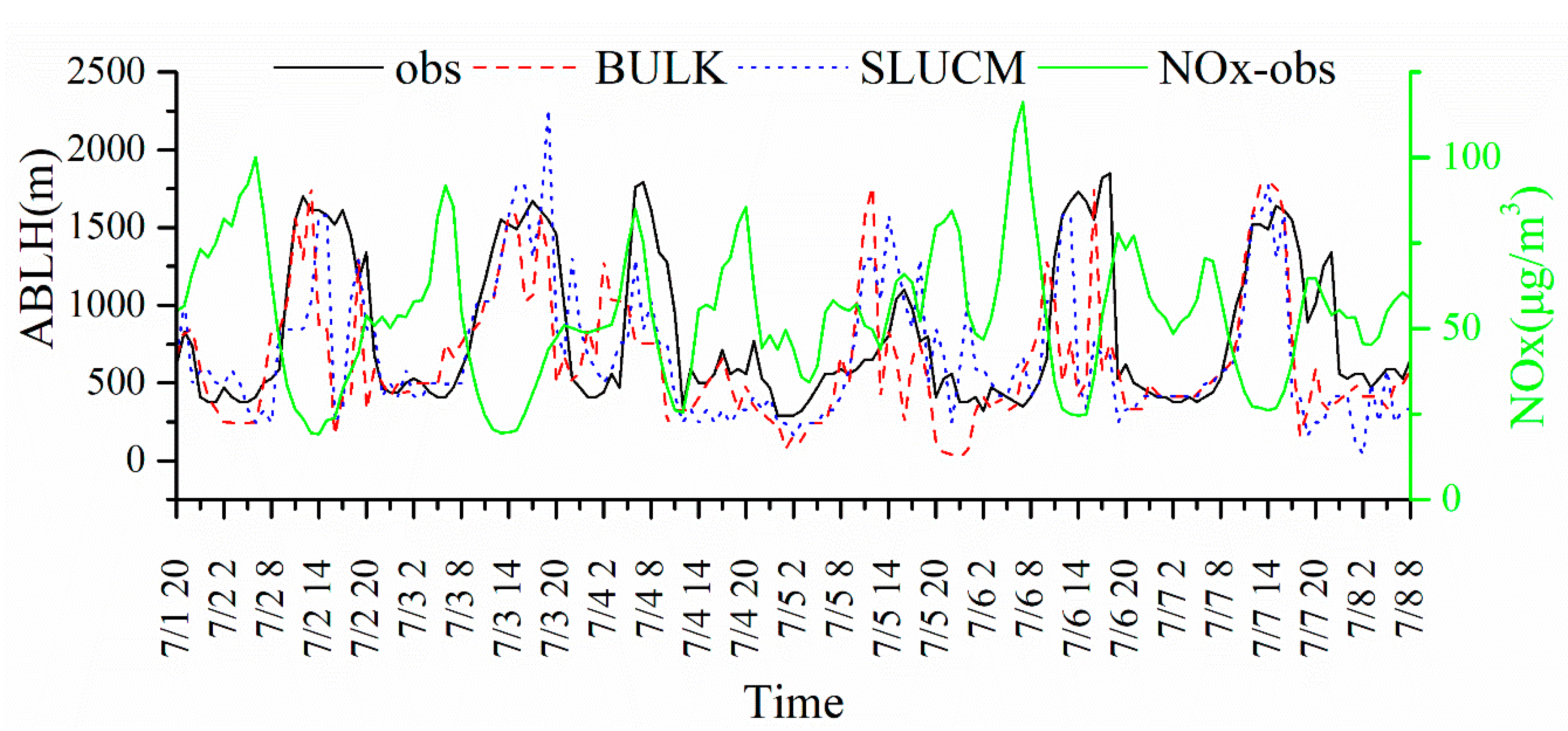
Figure 6 shows the observed and simulated ABLH values at station s2 on 1–8 July 2011. The observed data revealed that the ABLH on non-cold front days exhibited the well-known diurnal variation. As shown in Figure 5, the concentration of pollutants (except for PM_2.5) remained at low levels between 8:00 a.m. and 8:00 p.m. and at high values between 8:00 p.m. and 8:00 a.m. the next day during the same period, indicating that the pollutant concentration was correlated well with ABLH. For the ABLH, the model performed better during low-value periods than in high-value periods of diurnal variation. The duration of the simulated high values was low, and the values fluctuated significantly during the high-value periods. Scheme SLUCM showed no superiority over BULK during the regular diurnal variations. At 8:00 a.m. on 4 July, the cold front arrived, and the ABLH began to decrease until it reached a nadir at approximately 12:00 p.m. Then, it remained stable at approximately 500 m until 2:00 p.m. on 5 July. Between 2:00 and 8:00 p.m. on 5 July, a peak occurred at approximately 1000 m, far less than the normal daily peak at 1500 m; then, the ABLH was stable again at approximately 500 m until 8:00 a.m. on July 6. Scheme SLUCM accurately predicted the times that the ABLH began to decrease on 4 July and increase on 6 July, and it approximately predicted the peak between 2:00 and 8:00 p.m. on 5 July. The BULK scheme predicted that the ABLH would decrease four hours earlier and increase two hours earlier, and it predicted the ABLH peak on 5 July as occurring six hours earlier. From 8:00 p.m. on 5 July to 2:00 a.m. on 6 July, BULK predicted a virtual trough near 0 m, but SLUCM predicted a constant at approximately 500 m, which was more consistent with the observed values.

The MAGEs of BULK and SLUCM were 472.73 m and 431.95 m, respectively, and the correlation coefficients were 0.52 and 0.59, respectively. Scheme SLUCM decreased the MAGE by 40.78 m and increased the correlation coefficient by 0.07. Between 2:00 p.m. on 4 July and 8:00 a.m. on 6 July, the ABLH remained low. Between 2:00 p.m. on 4 July and 2:00 a.m. on 5 July, i.e., the first 10 h after the cold front arrived, the pollutant concentration remained low. The reason for this low concentration may be that the arrival of the cold front brought strong convective weather. From 2:00 a.m. on 5 July until 8:00 a.m. on 6 July, the pollutant concentration began to increase, and the NO_x and PM_2.5 levels remained high. Therefore, the pollutant concentration was correlated well with the ABLH during a cold front period, but strong wind and precipitation brought by a cold front may reduce pollution. In general, for the ABLH simulation, SLUCM performed better than BULK during the cold front period but did not show any superiority during the conventional diurnal variation period. Additionally, the pollutant concentration correlated well with the ABLH, indicating that SLUCM might perform better during high pollution periods.

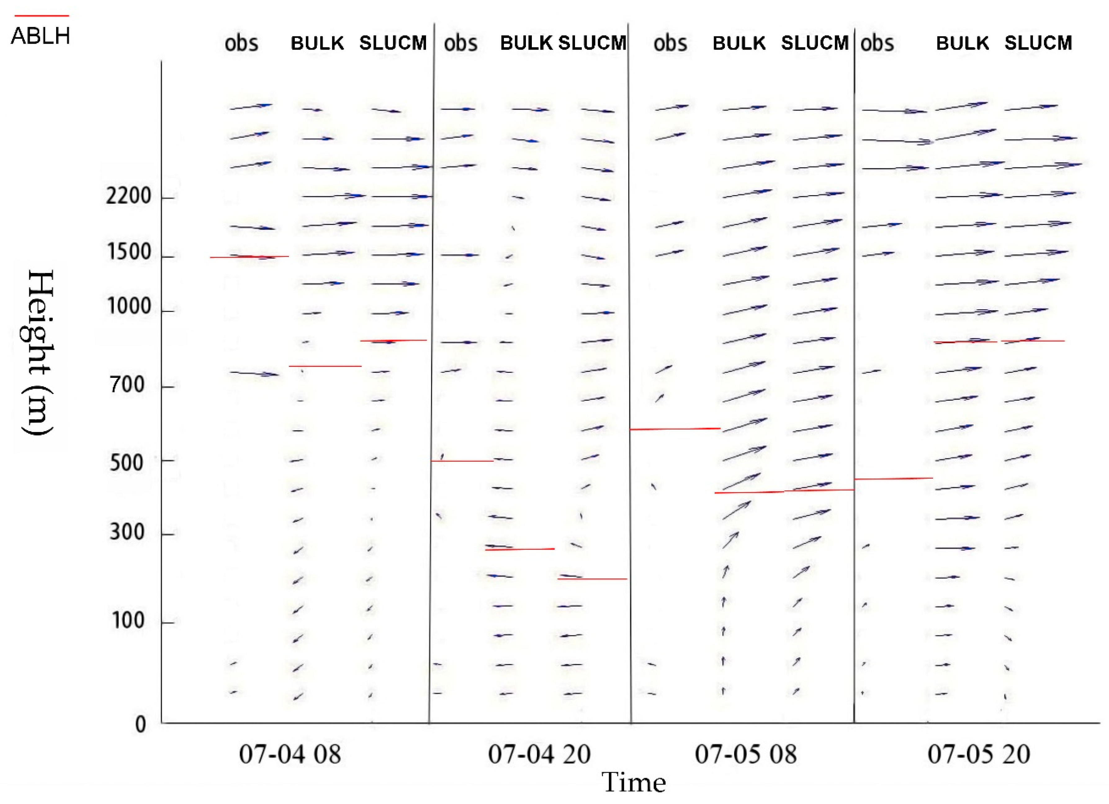
To compare the detailed vertical wind field during the cold front, the vertical wind profile obtained by radio soundings is shown with the model results at station s1 in Figure 7. The selected time is the moment of the greatest change in ABLH during the cold front. There were nulls at some heights because the data from the radio soundings below 2000 m were low-resolution. The simulated wind field from the ground to a high altitude showed a change from a northeasterly wind to a westerly wind at 8:00 a.m. on 4 July. Near the surface (0–100 m), the observed wind speed was low, and the wind direction was southwesterly. The simulated wind direction was northeasterly, and BULK overestimated the wind speed. At approximately 800 m, the observed wind direction changed to a westerly wind. The BULK-simulated wind was still in the process of changing direction because the wind speed approached 0 m/s, but the SLUCM-simulated wind direction had already changed to a westerly wind with the wind speed being closer to the measured wind speed. This result indicates that, at this moment, SLUCM better predicted the vertical change in the wind direction. At 8:00 p.m. on 4 July, both the observed and simulated wind directions changed from an easterly wind on the ground to a westerly wind at high altitudes. Between 200 and 800 m, the observed wind entirely finished the shift in direction, and SLUCM predicted this process well. At 800 m, the wind direction of SLUCM completely changed to a westerly wind, and the wind speed was close to the observed value. At this time and height, the wind direction predicted by BULK was still easterly. The SLUCM scheme was better than the BULK scheme at 8:00 p.m. on 4 July. At 8:00 a.m. on 5 July, the observed wind direction from the ground to a high altitude changed from easterly to westerly. The two schemes did not perform well at this moment in time. The predicted height of the change in wind direction was lower than the observation, and the simulated wind speed at the high altitude was larger than the observed speed. At 8:00 p.m. on 5 July, the wind changed from a southerly wind on the ground to a westerly wind at a high altitude. Neither scheme reproduced the change in wind direction well at this moment. Scheme BULK overestimated the wind speed, and SLUCM performed better than BULK. In general, for vertical wind simulations between 200 and 1000 m, SLUCM performed better than BULK. The data in Figure 7 and Table 3 show that SLUCM simulated the wind better than BULK for the 200–1000 m vertical heights in urban areas; however, on the ground, BULK performed better. The reason for this difference may be that the urban parameters are not sufficiently comprehensive. Although SLUCM considers the overall urban morphology, the available parameters were not accurate enough to represent the actual urban situation. Default values were used for parameters such as ε, α, and z₀ in Table 2 due to the lack of local data. This may have caused errors that exceeded the improvement in the wind simulation on the ground due to SLUCM. However, the improvement that SLUCM adds to the simulation is apparent as the errors from the buildings disappeared between 200 and 1000 m. Overall, SLUCM is recommended in urban areas to effectively simulate the wind field above the urban canopy, which shows the city morphology has a strong impact on the vertical wind field simulation of WRF. Given sufficiently accurate land use data, SLUCM may simulate the wind field in the entire boundary layer better than BULK.

4.4. Comparison of the Surface Temperature Fields

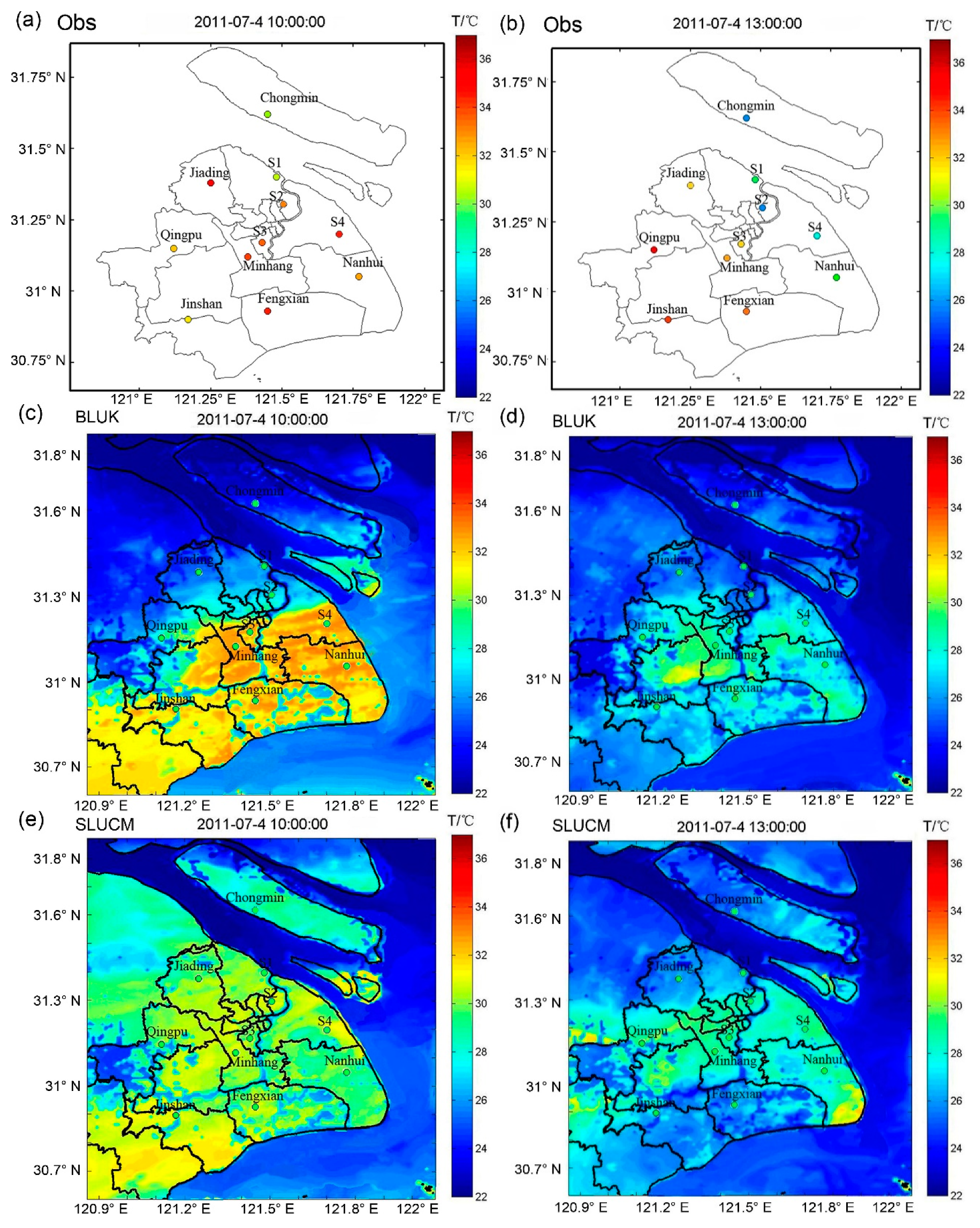
Figure 8 shows the observed air temperature at the 11 sites in Shanghai and the simulated air temperature field over Shanghai at 10:00 and 13:00 on 4 July 2011. The seven sites (except s1, s2, s3, and s4) shown in Figure 8 were used as supplemental sites for comparison of the temperature recordings. The observed temperatures at Chongming, s1, s2, and s4 began to decrease at 10:00 a.m. on 4 July, and the cooling process continued until 3:00 p.m. when the temperature dropped to 26 °C. The observed temperatures at all sites showed that the cold front arrived north of Shanghai during the time period between 10:00 and 11:00 a.m. and that the temperatures then decreased from the north to the south of Shanghai, with the cooling continuing for five hours. The BULK scheme predicted a significant frontal surface at 10:00 and 11:00 a.m. At 1:00 p.m., the cold front covered all of Shanghai, and the temperature did not decrease significantly after 1:00 p.m. At Chongming, Jiading, s1, and s2, the temperature began to decrease at 10:00 a.m. The cold front simulated by SLUCM arrived north of Shanghai at 10:00 a.m.; however, the edge of the cold front was not clear. During the time period between 10:00 and 11:00 a.m., the temperature north of Shanghai began to decrease, and cooling persisted for more than four hours, i.e., until 3:00 p.m. At Chongming, Jiading, and s1, the temperature began to decrease at 10:00 a.m. SLUCM more realistically simulated the time of the arrival of the cold front, thus predicting the movement of the cold front.

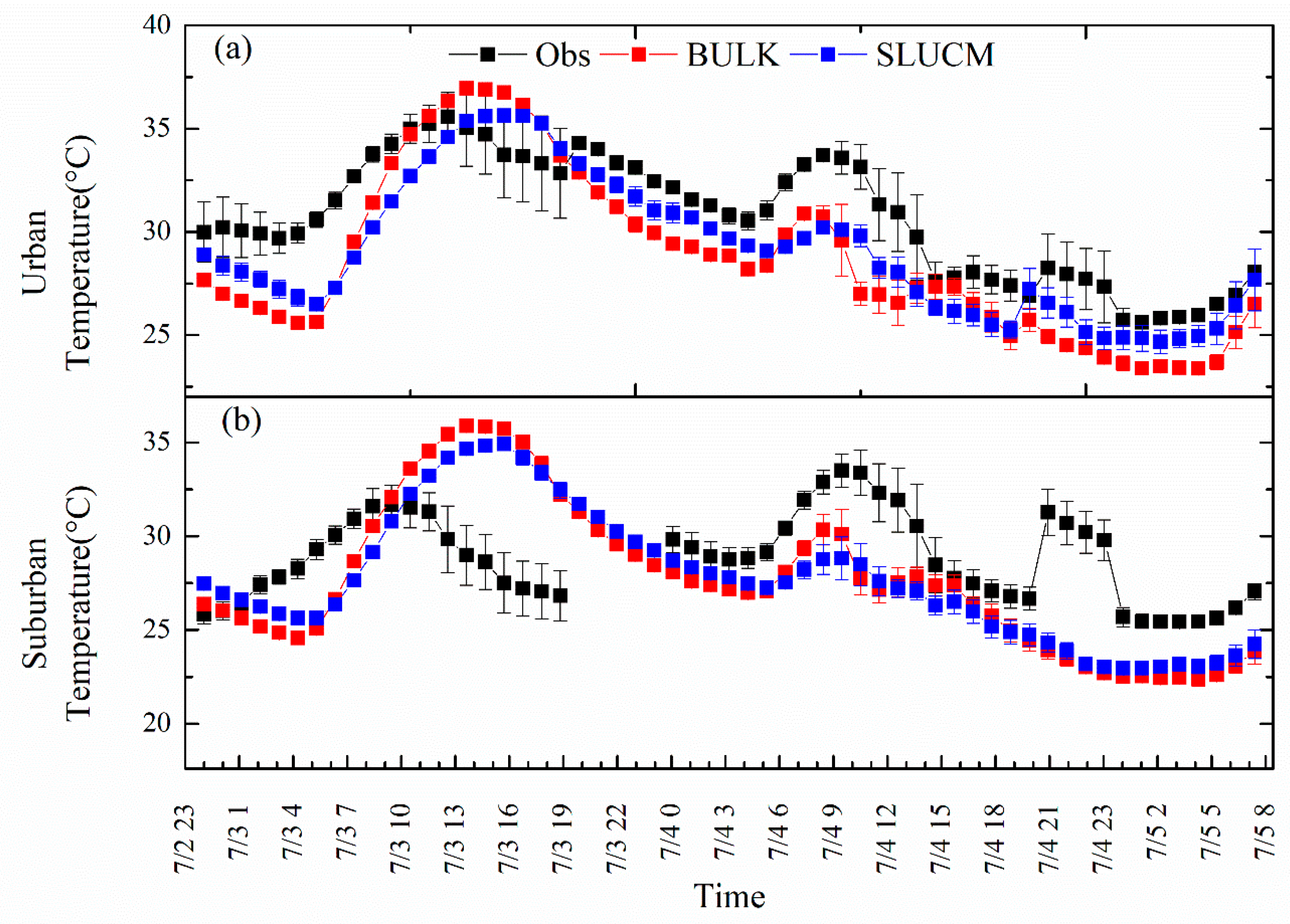
Figure 9 shows that the time series of temperatures during the cold front passed over Shanghai at 11 sites divided into two areas: (1) urban sites containing s1, s2, s3, and Minhang; and (b) suburban sites containing s4, Nanhui, Qingpu, Chongming, Jinshan, and Fengxian. The cold front simulated by BULK cooled significantly faster than what was observed. The spatial field of temperatures simulated by SLUCM is much closer to the observed temperatures. Additionally, the advantage of SLUCM on temperature simulation was more obvious in urban areas. The change in temperatures was closer to the observed temperatures and the absolute error was smaller. The cooling process simulated by SLUCM was closer to the observations. In general, SLUCM simulated the cooling process better than BULK during the passage of the cold front. The reason for this improvement might be that the urban canopy layer increases the surface roughness of the Shanghai metropolitan area, slowing the advance of the cold front. Without considering the urban canopy, BULK simulated a more rapidly cooling cold front, and SLUCM simulated the cooling closer to the actual measurements by considering the urban canopy.

4.5. Comparison of the Concentrations of Air Pollutants

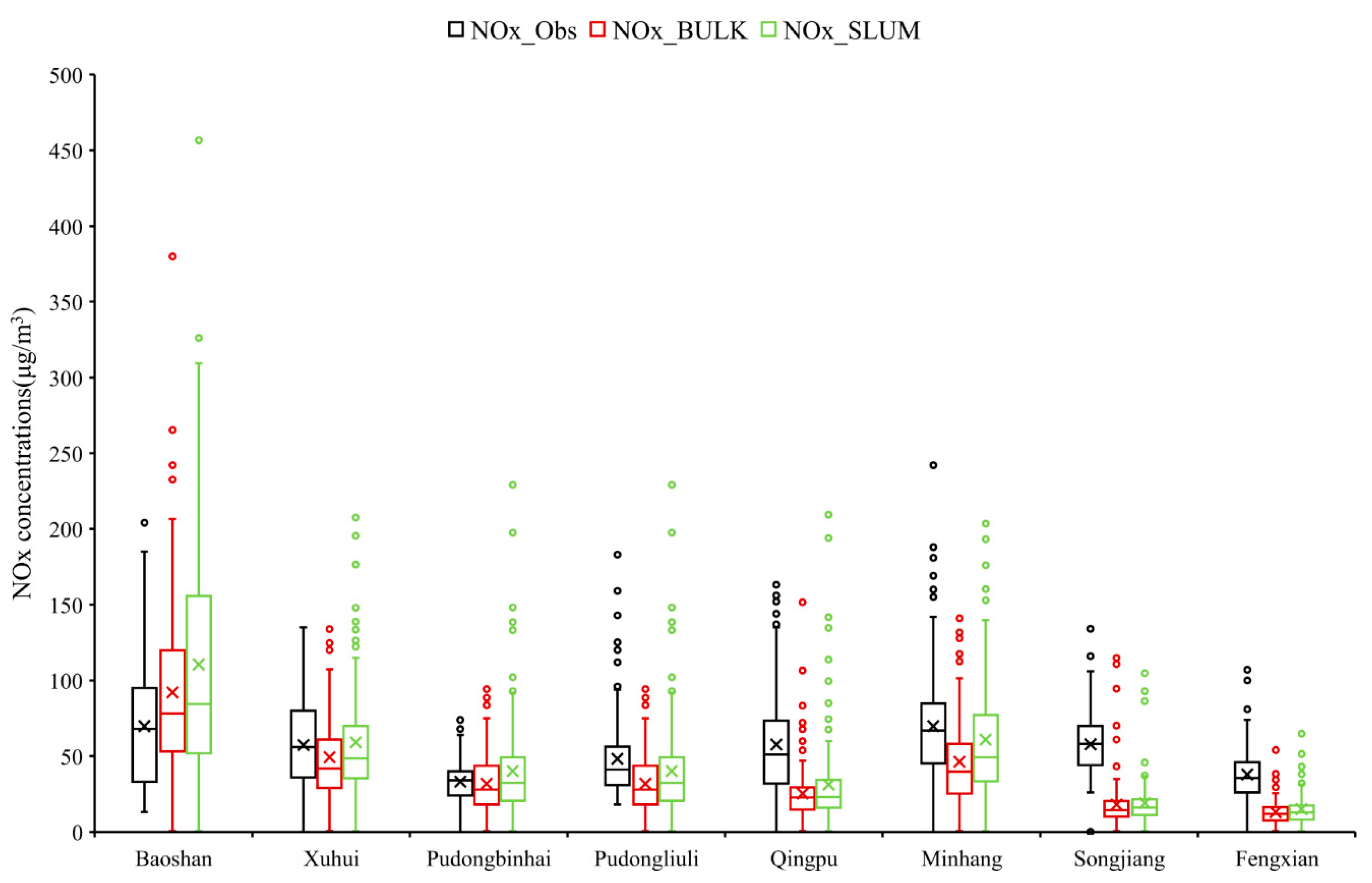
In terms of the effect of meteorological conditions on pollutant concentrations, we used NOx as an example to show the influence of urban scheme on the simulation of air quality. The observed and simulated mean concentrations of NO_x at eight stations on 1–8 July 2011 are shown in Figure 10. The seven sites (except Baoshan) shown in Figure 11 were used as supplemental sites for a comparison of the concentrations of air pollutants. This shows that different urban schemes influence NO_x. At most sites, SLUCM simulations performed better than the BULK scheme. the simulated concentrations at urban sites like Xuhui and Minhang were obviously improved by WRF-SLUCM-CMAQ. The NOx concentration determined by SLUCM (59.3 μg/m³ at Xuhui and 60.9 μg/m³ at Minhang) was much closer to the observations (57.4 μg/m³ at Xuhui and 68.4 μg/m³ at Minhang) than BULK (49.4 μg/m³ at Xuhui and 46.2 μg/m³ at Minhang).

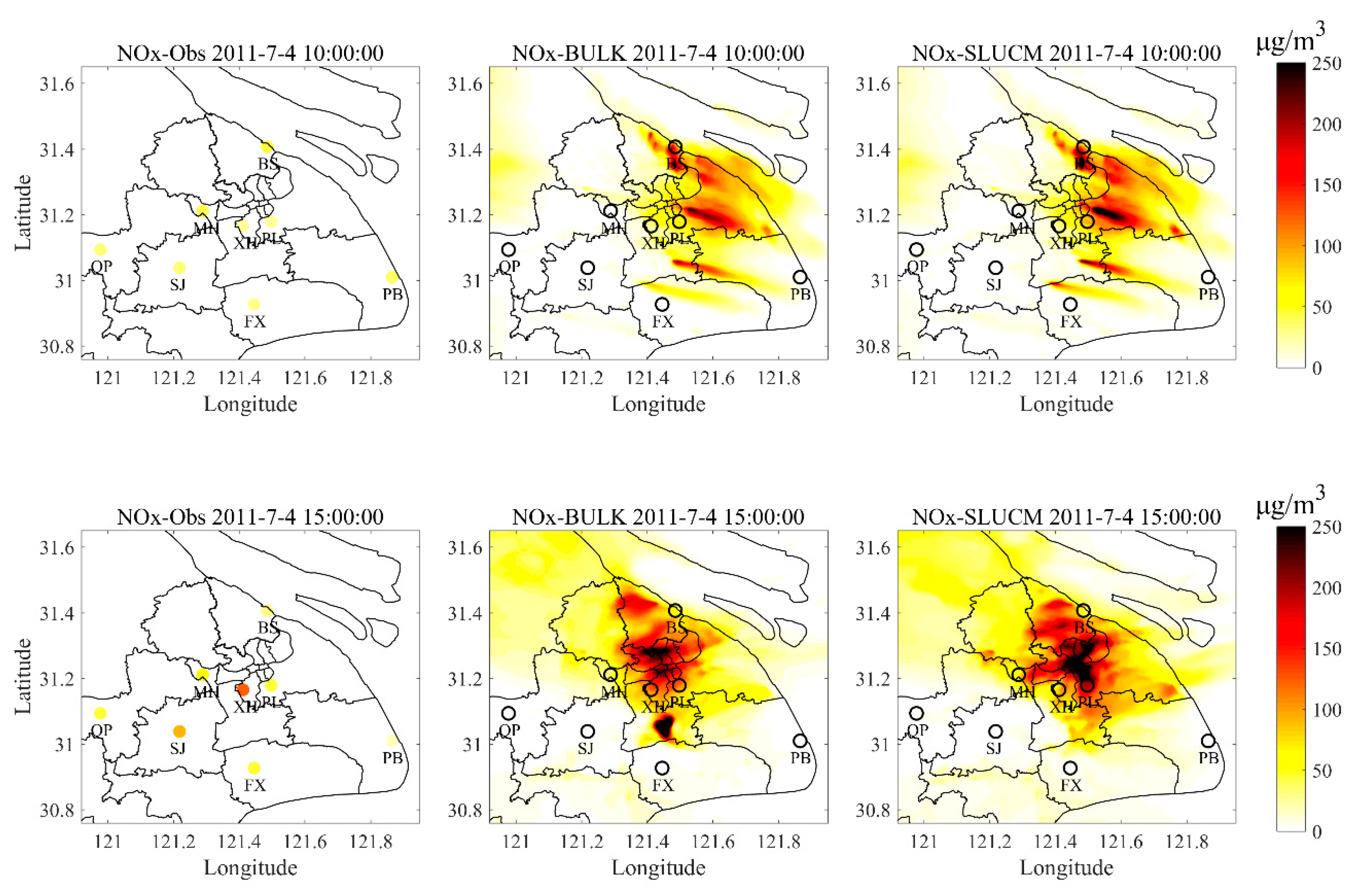
The simulated spatial field and observed NO_x concentrations at eight sites in Shanghai with the arrival of the cold front on 4 July 2011 at 10:00 a.m. and 3:00 p.m. are shown in Figure 11 to demonstrate the response of air pollutants to WRF-SLUCM/CMAQ. WRF-CMAQ of BULK and SLUCM both simulated the delayed arrival of the cold front leading to a slow response to the change in air pollutants with the cold front. The simulated concentration of NO_x in the area surrounding the Baoshan site was still high at 10:00 a.m. but the observations dropped below 50 μg/m³. However, the prediction is more realistic in that the large point-source pollutants in the north of Shanghai diffused more slowly toward the south with the SLUCM scheme compared to with the BULK scheme. At 3:00 to 4:00 p.m., the simulated concentration of NO_x was dropping in some sites, like the Minhang site, in WRF-BULK-CMAQ; however, the simulated concentration of NO_x was still in the high value area in WRF-SLUCM-CMAQ, which is closer to the observation of 150 μg/m³ at the Minhang site. Overall, the reduction in wind speed and the boundary layer due to the barrier role of the urban area that led to a wider polluted urban area and higher concentration was demonstrated by WRF-SLUCM-CMAQ compared with WRF-BULK-CMAQ, which is closer to the observation during the cold front.

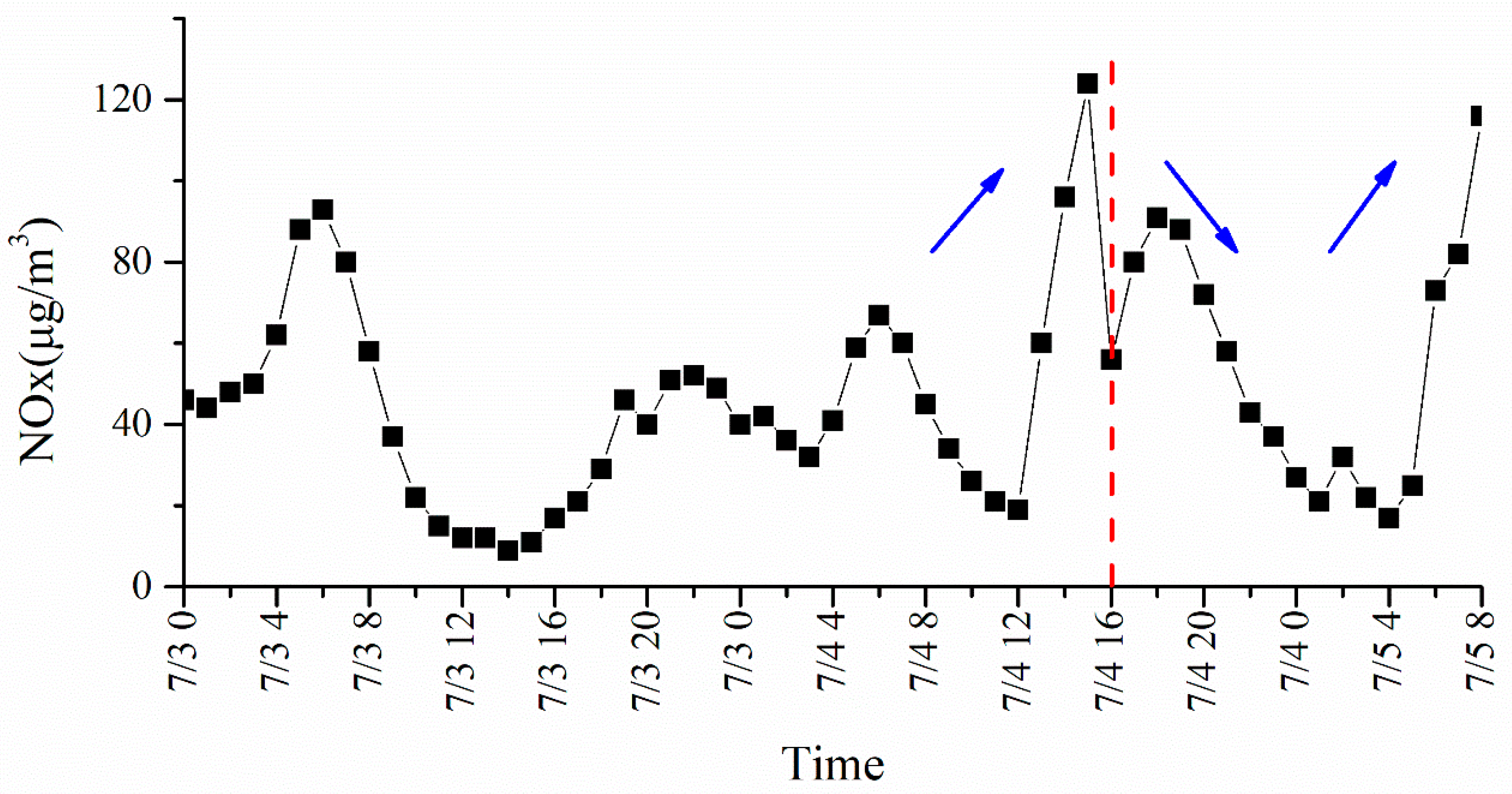
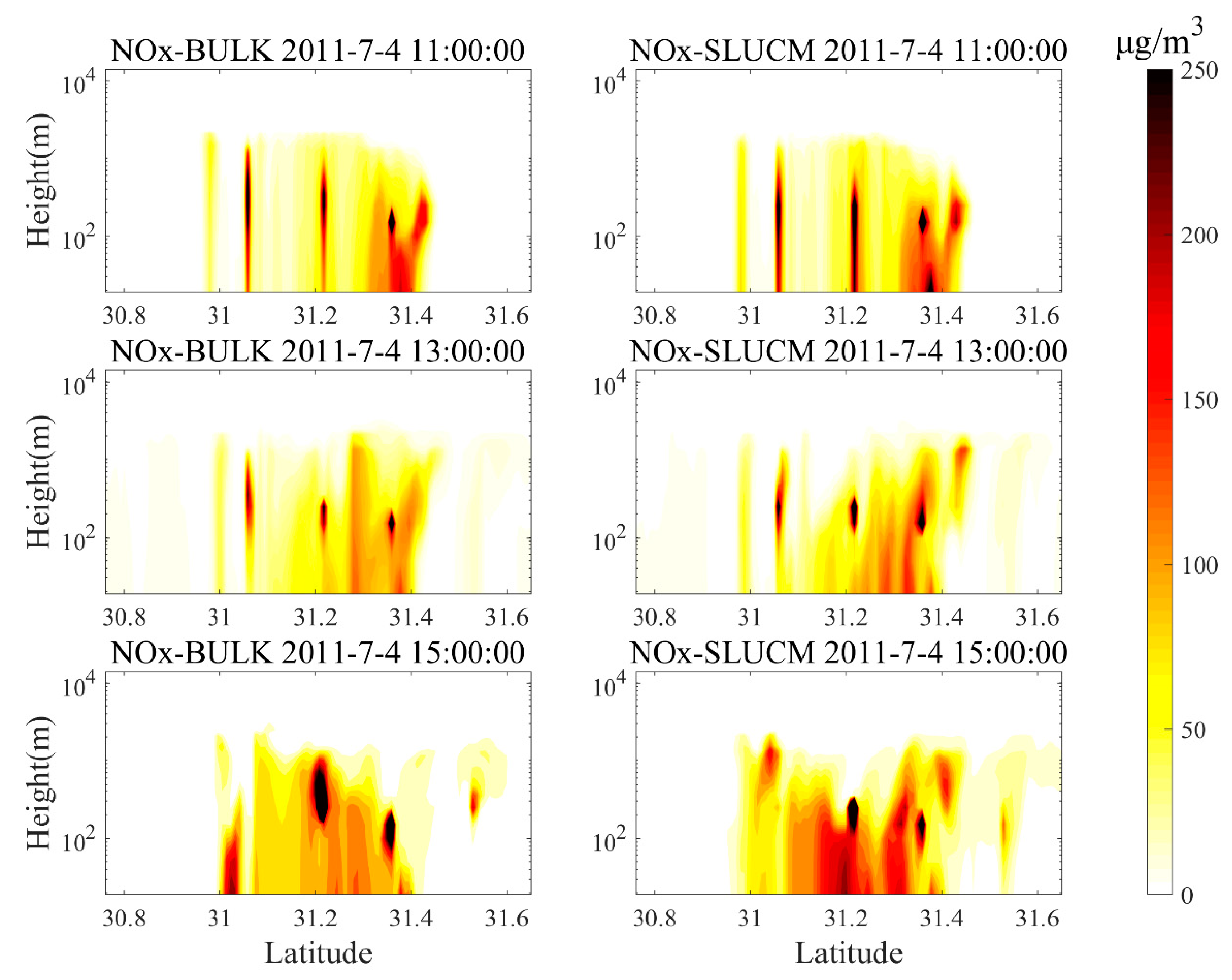
Figure 12 shows that the time series of NO_x concentrations on 3–5 July. The results in Figure 12 show that the observed concentrations rose right before the arrival of the cold front and then declined continuously during the cold front. Due to the northerly wind, the cold front was coming from the north of Shanghai, where the Baoshan site is located. NO_x concentration declined with the cold front arrival at 10:00 a.m. Simultaneously, the area influenced by the northerly winds expanded with the moving of the cold front. The Xuhui site was directly downstream from the cold front at this moment; the concentration of NO_x there increased and continued to increase to 124 μg/m³ at 2:00 p.m. Subsequently, NO_x concentration decreased during the cold front passing the Xuhui site. Figure 13 shows vertical cross sections of simulated NO_x concentrations along the longitude 121.4° E during the process of the cold front passing. It reveals again that surface NO_x tended toward high concentrations before the cold front, significantly decreasing as the cold front passed, and had higher concentrations after the cold front had passed by. The results are similar to those reported by Cheng et al. [25]. At 10:00 a.m., the cold front passed the Baoshan site with the Minhang site downstream from the cold front. The high NO_x concentration lifted to the upper atmosphere, which appeared to form hotspots around 500 m at the Baoshan site, while the concentration rose at the Minhang site. At 12:00–1:00 p.m., the cold front covered Shanghai, the surface NO_x concentration rapidly decreased, and high NO_x concentrations lifted to the upper air layer. After the cold front passed the Xuhui site, the NO_x concentration increased to a higher value at around 2:00–3:00 p.m. Both WRF-SLUCM-CMAQ and WRF-BULK-CMAQ simulated similar vertical variations with the passage of a cold front, but the results using WRF-SLUCM-CMAQ were much more accurate.

5. Conclusions

In this study, the BULK and SLUCM schemes were implemented in WRF-CMAQ to analyze their simulation performance of urban meteorology and pollutant changes for the entire Shanghai area. For meteorological aspects including air temperature, wind speed, relative humidity, and ABLH, the simulations performed by the SLUCM scheme were better than the BULK scheme. The SLUCM scheme simulations were closer to the actual observations than the BULK scheme simulations. The SLUCM scheme simulations decreased the mean wind speed by 0.7 m s⁻¹, increased the mean temperature by up to 0.8 °C, and increased the mean ABLH by up to 37 m. For both schemes, the simulated and observed values of temperature and relative humidity were well correlated. The SLUCM scheme better simulated changing trends to predict the ABLH but did not accurately simulate the wind speed or wind direction. The SLUCM simulation was better for the air temperature, wind speed, relative humidity, and ABLH, but did not work well for wind direction. For the concentration field of air pollutants, the simulation results using the SLUCM scheme performed comparatively better than those using the BULK scheme. The SLUCM scheme predicted a wider area of pollution than the BULK scheme, and the concentrations were closer to the values observed using the SLUCM scheme.

The SLUCM simulation performed significantly better than the BULK simulation for the daily minimum temperature predictions, especially in urban areas. However, for the daily maximum temperature simulations, SLUCM did not perform better than BULK. The improvement in the temperature simulation achieved using SLUCM was more effective at higher urbanization levels. The SLUCM scheme performed better for the mean relative humidity simulation, especially in LIR areas. However, the improvement in the relative humidity simulation by the SLUCM scheme was greater in the HIR areas than in the LIR areas. The implementation of SLUCM reduced the virtual peak that occurred in the wind speed simulation. The greatest improvement in the wind speed simulation by the implementation of SLUCM occurred in the rural areas. However, the SLUCM scheme did not show more merit than the BULK scheme for wind direction simulations in the rural and HIR areas. However, the SLUCM scheme performed better in the LIR areas. For the ABLH simulations, the SLUCM scheme performed better than the BULK scheme during a cold front episode but was not better for conventional diurnal variations. The SLUCM scheme better simulated wind than the BULK scheme for the vertical layers between 200 and 1000 m in urban areas, but on the ground, the BULK scheme performed better. The SLUCM scheme exhibited advantages when the errors from buildings disappeared between 200 and 1000 m. Therefore, in urban areas, SLUCM is the recommended scheme to apply with localized urban parameters to effectively simulate the wind field above the urban canopy. During the passage of the cold front, SLUCM predicted the arrival time of the cold front and more realistically simulated the moving cold front. The cooling process simulated by SLUCM was closer to the observation than that simulated by BULK. The barrier role of the urban canopy during a cold front was better represented by SLUCM than by BULK.

For the pollutant concentration field, the mean values predicted by the SLUCM scheme were closer to the observations at urban sites. The barrier role of the urban area led to a wider polluted urban area and a higher concentration being predicted by SLUCM than by BULK, which is closer to the observations during the cold front.

The limitations of the urban parameters in Shanghai can limit the simulation accuracy of the SLUCM scheme. Given sufficiently accurate land use data, the SLUCM scheme can simulate the wind field in the entire boundary layer better than the BULK scheme, which then affects the precision of the pollutant concentration simulation.

References

1. Zhang, H.; Zhou, L.G.; Chen, M.N.; Ma, W.C. Land Use Dynamics of the Fast-Growing Shanghai Metropolis, China (1979–2008) and its Implications for Land Use and Urban Planning Policy. Sensors 2011, 11, 1794–1809. [Google Scholar] [CrossRef] [PubMed] [Green Version]
2. Lin, T.J.; Xuan, C. The National Development and Reform Commission of China. The National New Urbanization Report 2015; China Planning Press: Beijing, China, 2016; Chapter 3. [Google Scholar]
3. Cui, L.; Shi, J. Urbanization and its environmental effects in Shanghai, China. Urban Clim. 2012, 2, 1–15. [Google Scholar] [CrossRef] [Green Version]
4. Zhang, C.L.; Chen, F.; Miao, S.G.; Li, Q.C.; Xia, X.A.; Xuan, C.Y. Impacts of urban expansion and future green planting on summer precipitation in the Beijing metropolitan area. J. Geophys. Res. Atmos. 2009, 114, D02116. [Google Scholar] [CrossRef]
5. Wang, X.M.; Lin, W.S.; Yang, L.M.; Deng, R.R.; Lin, H. A numerical study of influences of urban land-use change on ozone distribution over the Pearl River Delta region, China. Tellus Series B Chem. Phys. Meteorol. 2007, 59, 633–641. [Google Scholar] [CrossRef] [Green Version]
6. Gao, Z.; Bian, L. Estimation of aerodynamic roughness length and displacement of an urban surface from single-level sonic anemometer data. Australian Meteorol. Mag. 2004, 54, 21–28. [Google Scholar]
7. Xu, Y.; Liu, S.; Hu, F.; Ma, N.; Wang, Y.; Shi, Y.; Jia, H. Influence of Beijing urbanization on the characteristics of atmospheric boundary layer. Chin. J. Atmos. Sci. 2009, 33, 859–867. [Google Scholar]
8. Zhan, W.J.; Zhang, Y.; Ma, W.C.; Yu, Q.; Chen, L.M. Estimating influences of urbanizations on meteorology and air quality of a Central Business District in Shanghai, China. Stoch. Environ. Res. Risk Assess. 2013, 27, 353–365. [Google Scholar] [CrossRef]
9. Zhang, N.; Gao, Z.; Wang, X.; Chen, Y. Modeling the impact of urbanization on the local and regional climate in Yangtze River Delta, China. Theor. Appl. Climatol. 2010, 102, 331–342. [Google Scholar] [CrossRef]
10. Cheng, F.Y.; Chin, S.C.; Liu, T.H. The role of boundary layer schemes in meteorological and air quality simulations of the Taiwan area. Atmos. Environ. 2012, 54, 714–727. [Google Scholar] [CrossRef]
11. Lee, S.H.; Kim, S.W.; Angevine, W.M.; Bianco, L.; McKeen, S.A.; Senff, C.J.; Trainer, M.; Tucker, S.C.; Zamora, R.J. Evaluation of urban surface parameterizations in the WRF model using measurements during the Texas Air Quality Study 2006 field campaign. Atmos. Chem. Phys. 2011, 11, 2127–2143. [Google Scholar] [CrossRef] [Green Version]
12. Yu, S.; Mathur, R.; Pleim, J.; Pouliot, G.; Wong, D.; Eder, B.; Schere, K.; Gilliam, R.; Rao, S.T. Comparative evaluation of the impact of WRF/NMM and WRF/ARW meteorology on CMAQ simulations for PM2.5 and its related precursors during the 2006 TexAQS/GoMACCS study. Atmos. Chem. Phys. 2012, 12, 4091–4106. [Google Scholar] [CrossRef] [Green Version]
13. Kusaka, H.; Kondo, H.; Kikegawa, Y.; Kimura, F. A simple single-layer urban canopy model for atmospheric models: Comparison with multi-layer and slab models. Bound. Layer Meteorol. 2001, 101, 329–358. [Google Scholar] [CrossRef]
14. Holt, T.; Pullen, J. Urban Canopy Modeling of the New York City Metropolitan Area: A Comparison and Validation of Single- and Multilayer Parameterizations. Mon. Weather Rev. 2007, 135, 1906–1930. [Google Scholar] [CrossRef]
15. Zhang, N.; Zhu, L.; Zhu, Y. Urban heat island and boundary layer structures under hot weather synoptic conditions: A case study of Suzhou City, China. Adv. Atmos. Sci. 2011, 28, 855–865. [Google Scholar] [CrossRef]
16. Miao, S.; Chen, F.; Lemone, M.A.; Tewari, M.; Li, Q.; Wang, Y. An Observational and Modeling Study of Characteristics of Urban Heat Island and Boundary Layer Structures in Beijing. J. Appl. Meteorol. Climatol. 2009, 48, 484–501. [Google Scholar] [CrossRef]
17. Jung, J.; Lee, H.; Kim, Y.J.; Liu, X.; Zhang, Y.; Gu, J.; Fan, S. Aerosol chemistry and the effect of aerosol water content on visibility impairment and radiative forcing in Guangzhou during the 2006 Pearl River Delta campaign. J. Environ. Manag. 2009, 90, 3231–3244. [Google Scholar] [CrossRef] [PubMed]
18. Xiao, R.; Takegawa, N.; Kondo, Y.; Miyazaki, Y.; Miyakawa, T.; Hu, M.; Shao, M.; Zeng, L.M.; Hofzumahaus, A.; Holland, F.; et al. Formation of submicron sulfate and organic aerosols in the outflow from the urban region of the Pearl River Delta in China. Atmos. Environ. 2009, 43, 3754–3763. [Google Scholar] [CrossRef]
19. Lu, K.; Zhang, Y.; Su, H.; Shao, M.; Zeng, L.; Zhong, L.; Xiang, Y.; Chang, C.; Chou, C.K.C.; Wahner, A. Regional ozone pollution and key controlling factors of photochemical ozone production in Pearl River Delta during summer time. Sci. China Chem. 2010, 53, 651–663. [Google Scholar] [CrossRef]
20. Zhang, Y.H.; Hu, M.; Zhong, L.J.; Wiedensohler, A.; Liu, S.C.; Andreae, M.O.; Wang, W.; Fan, S.J. Regional Integrated Experiments on Air Quality over Pearl River Delta 2004 (PRIDE-PRD2004): Overview. Atmos. Environ. 2008, 42, 6157–6173. [Google Scholar] [CrossRef]
21. Zhang, Y.H.; Su, H.; Zhong, L.J.; Cheng, Y.F.; Zeng, L.M.; Wang, X.S.; Xiang, Y.R.; Wang, J.L.; Gao, D.F.; Shao, M. Regional ozone pollution and observation-based approach for analyzing ozone–Precursor relationship during the PRIDE-PRD2004 campaign. Atmos. Environ. 2008, 42, 6203–6218. [Google Scholar] [CrossRef]
22. Rose, D.; Nowak, A.; Achtert, P.; Wiedensohler, A.; Hu, M.; Shao, M.; Zhang, Y.; Andreae, M.O.; Poschl, U. Cloud condensation nuclei in polluted air and biomass burning smoke near the mega-city Guangzhou, China—Part 1: Size-resolved measurements and implications for the modelling of aerosol particle hygroscopicity and CCN activity. Atmos. Chem. Phys. 2010, 10, 3365–3383. [Google Scholar] [CrossRef]
23. Cheng, Y.F.; Wiedensohler, A.; Eichler, H.; Heintzenberg, J.; Tesche, M.; Ansmann, A.; Wendisch, M.; Su, H.; Althausen, D.; Herrmann, H.; et al. Relative humidity dependence of aerosol optical properties and direct radiative forcing in the surface boundary layer at Xinken in Pearl River Delta of China: An observation based numerical study. Atmos. Environ. 2008, 42, 6373–6397. [Google Scholar] [CrossRef]
24. Fan, S.J.; Fan, Q.; Yu, W.; Luo, X.Y.; Wang, B.M.; Song, L.L.; Leong, K.L. Atmospheric boundary layer characteristics over the Pearl River Delta, China, during the summer of 2006: Measurement and model results. Atmos. Chem. Phys. 2011, 11, 6297–6310. [Google Scholar] [CrossRef]
25. Cheng, N.L.; Meng, F.; Xu, J.; He, Y.J. Process analysis about the impact of a strong cold front on air pollution transportation in Eastern China in spring. Res. Environ. Sci. 2013, 26, 34–42. [Google Scholar]
26. Shahgedanova, M.; Burt, T.P.; Davies, T.D. Synoptic Climatology of Air Pollution in Moscow. Theor. Appl. Climatol. 1998, 61, 85–102. [Google Scholar] [CrossRef]
27. Carmichael, G.R.; Peters, L.K.; Saylor, R.D. The STEM-II regional scale acid deposition and photochemical oxidant model—I. An overview of model development and applications. Atmos. Environ. Part B Urban Atmos. 1991, 25, 25–45. [Google Scholar] [CrossRef]
28. Wang, S.; Yang, D.; Li, L.; Huang, J.; Qi, B. Cold-front activities and its influence on air pollution at urban districts of Lanzhou in cold half year. Plateau Meteorol. 1998, 17, 142–149. [Google Scholar]
29. Skamarock, W.C.; Klemp, J.B.; Dudhia, J.; Gill, D.O.; Barker, D.M.; Duda, M.G.; Huang, X.-Y.; Wang, W.; Powers, J.G. A Description of the Advanced Research WRF Version 3; National Centre of Atmospheric Research: Boulder, CO, USA, 2008. [Google Scholar]
30. Byun, D.; Ching, J. Science Algorithms of the EPA Models-3 Community Multiscale Air Quality (CMAQ) Modeling System; US Environmental Protection Agency: Washington, DC, USA, 1999; EPA-600/R-99/030.
31. Byun, D.; Schere, K.L. Review of the governing equations, computational algorithms, and other components of the models-3 community multiscale air quality (CMAQ) modeling system. Appl. Mech. Rev. 2006, 59, 51–77. [Google Scholar] [CrossRef]
32. Tan, J.N.; Yu, Q.; Ma, W.C.; Ma, J.L.; Zhang, Y.; Cheng, J. Development of refined emission inventory of air pollutants: A case study of shanghai baoshan district. Acta Sci. Circumst. 2014, 34, 1099–1108. [Google Scholar]
33. Tan, J.N.; Zhang, Y.; Ma, W.C.; Yu, Q.; Wang, J.; Chen, L.M. Impact of spatial resolution on air quality simulation: A case study in a highly industrialized area in Shanghai, China. Atmos. Pollut. Res. 2015, 6, 322–333. [Google Scholar] [CrossRef] [Green Version]
34. Chen, F.; Kusaka, H.; Bornstein, R.; Ching, J.; Grimmond, C.S.B.; Grossman-Clarke, S.; Loridan, T.; Manning, K.W.; Martilli, A.; Miao, S.G.; et al. The integrated WRF/urban modelling system: development, evaluation, and applications to urban environmental problems. Int. J. Climatol. 2011, 31, 273–288. [Google Scholar] [CrossRef] [Green Version]
35. Liu, X.; Cheng, Y.; Zhang, Y.; Jung, J.; Sugimoto, N.; Chang, S.Y.; Kim, Y.J.; Fan, S.; Zeng, L. Influences of relative humidity and particle chemical composition on aerosol scattering properties during the 2006 PRD campaign. Atmos. Environ. 2008, 42, 1525–1536. [Google Scholar] [CrossRef]
36. Kusaka, H.; Kimura, F. Coupling a single-layer urban canopy model with a simple atmospheric model: Impact on urban heat island simulation for an idealized case. J. Meteorol. Soc. Jpn. 2004, 82, 67–80. [Google Scholar] [CrossRef]
37. Kusaka, H.; Kimura, F. Thermal effects of urban canyon structure on the nocturnal heat island: Numerical experiment using a mesoscale model coupled with an urban canopy model. J. Appl. Meteorol. 2004, 43, 1899–1910. [Google Scholar] [CrossRef]
38. Salamanca, F.; Martilli, A.; Tewari, M.; Chen, F. A Study of the Urban Boundary Layer Using Different Urban Parameterizations and High-Resolution Urban Canopy Parameters with WRF. J. Appl. Meteorol. Climatol. 2011, 50, 1107–1128. [Google Scholar] [CrossRef]
39. Ouermi, T.A.J.; Knoll, A.; Kirby, R.M.; Berzins, M. Optimization Strategies for WRF Single-Moment 6-Class Microphysics Scheme (WSM6) on Intel Microarchitectures. In Proceedings of the 2017 Fifth International Symposium on Computing and Networking (CANDAR), Aomori, Japan, 19–22 November 2017; IEEE Computer Society: Salt Lake City, UT, USA, 2018; pp. 146–152. [Google Scholar] [CrossRef]
40. Zhang, Y.; Zhan, W.J.; Ma, W.C.; Yu, Q.; Chen, L.M. Sensitivity analysis of meteorological conditions and air pollution concentration on land-use data in the YRD region. J. Nanjing Univ. (Nat. Sci.) 2015, 51, 562. [Google Scholar] [CrossRef]
41. Yu, S.; Eder, B.; Dennis, R.; Chu, S.H.; Schwariz, S. On the development of new metrics for the evaluation of air quality models. Atmos. Sci. Lett. 2005, 7, 26–34. [Google Scholar] [CrossRef]
Figure 1. (a) Domain settings in the weather research and forecasting (WRF) model and (b) the measurement sites in Shanghai.
Atmosphere 10 00079 g001
Figure 2. The land use of Shanghai in (a) 1980 and (b) 2007.
Atmosphere 10 00079 g002
Figure 3. Shanghai hourly and daily mean temperature on 1–8 July 2011.
Atmosphere 10 00079 g003
Figure 4. Weather maps of East Asia at 2:00 a.m. and 2:00 p.m. UTC + 8 on 4 July and 5 July 2011. The maps are courtesy of the Korea Meteorological Administration.
Atmosphere 10 00079 g004
Figure 5. Observed pollutant concentrations in Shanghai on 1–8 July 2011.
Atmosphere 10 00079 g005
Figure 6. Observed and simulated ABL height (ABLH) at station s2 and average NOx concentrations in Shanghai on 1–8 July 2011.
Atmosphere 10 00079 g006
Figure 7. Vertical wind profile and ABLH measured by radio soundings and model results at station s1 at 8:00 and 20:00 on 4 July and 5 July 2011.
Atmosphere 10 00079 g007
Figure 8. Horizontal distributions of observed temperatures at 11 sites in Shanghai and simulated temperatures over Shanghai on 4 July 2011 (a) Observed temperatures at 10:00; (b) Observed temperatures at 13:00; (c) Simulated temperatures by BULK at 10:00; (d) Simulated temperatures by BULK at 13:00; (e) Simulated temperatures by SLUCM at 10:00; (f) Simulated temperatures by SLUCM at 13:00.
Atmosphere 10 00079 g008
Figure 9. Time series of temperatures as the cold front passed over Shanghai at 11 sites divided into two areas: (a) urban sites containing s1, s2, s3, and Minhang; (b) suburban sites containing s4, Nanhui, Qingou, Chongming, Jinshan, and Fengxian.
Atmosphere 10 00079 g009
Figure 10. Observed and simulated mean concentrations of eight stations on 1–8 July 2011.
Atmosphere 10 00079 g010
Figure 11. Horizontal distributions of the observed concentration of NOx at eight sites and simulated concentration of NOx field over Shanghai on 4 July 2011 at 10:00 a.m. and 3:00 p.m. BS: Baoshan; MH: Minhang; XH: Xuhui; PL: Pudongliuli; PB: Pudongbinhai; FX: Fengxian; SJ: Songjiang; QP: Qingpu.
Atmosphere 10 00079 g011
Figure 12. Time series of NOx concentration at Xuhui site on 3–5 July 2011. Red dash line: Cold front passing time.
Atmosphere 10 00079 g012
Figure 13. Vertical distribution of simulated NOx concentrations along the longitude 121.4° E during the process of the cold front passing.
Atmosphere 10 00079 g013