Distribution of Air Temperature Multifractal Characteristics Over Greece

Abstract

In this study, Multifractal Detrended Fluctuation Analysis (MF-DFA) is applied to daily temperature time series (mean, maximum and minimum values) from 22 Greek meteorological stations with the purpose of examining firstly their scaling behavior and then checking if there are any differences in their multifractal characteristics. The results showed that the behavior is the same at almost all stations, i.e., time series are positive long-term correlated and their multifractal structure is insensitive to local fluctuations with large magnitude. Moreover, this study deals with the spatial distribution of the main characteristics of multifractal (singularity) spectrum: the dominant Hurst exponent, the width of the spectrum, the asymmetry and the truncation type of the spectrum. The spatial distributions are discussed in terms of possible effects from various climatic features. In general, local atmospheric circulation and weather conditions are found to affect the shape of the spectrum and the corresponding spatial distributions. Furthermore, the intercorrelation of the main multifractal spectrum parameters resulted in a well-defined group of stations sharing similar multifractal characteristics. The results indicate the usefulness of the non-linear analysis in climate research due to the complex interactions among the natural processes.

1. Introduction

Complex systems consist of many components that interact with each other in very complicated ways, which are determined by nonlinear laws. A characteristic example of a complex system is the atmosphere and the natural processes that take place in it. The result of such complex interaction among atmospheric processes is the fluctuation of the values of meteorological parameters in an almost random way at many scales in time and space. These nonlinear processes are described by nonlinear partial differential equations [1]. Nonlinearity results in linear data analysis being insufficient for a complete analysis of meteorological time series. Besides atmospheric sciences, nonlinearity also occurs in many other fields of science such as economics, biology, physiology, electronics etc. [2]. Nowadays, the close cooperation of scientists from various disciplines has helped decisively in the development of new effective methods for the analysis of nonlinear phenomena. Researchers can now analyze processes that obey nonlinearity and they are able to reveal some properties, which could not be detected by linear methods. One such nonlinear method is Detrended Fluctuation Analysis (DFA), which was developed by [3]. It should be mentioned that the fluctuations of time series from complex systems obey scaling laws for a broad range of time (and space) scales. By applying DFA, we can reveal the scaling properties and determine long-range correlations, even in nonstationary time series [4]. This could not be done by using ordinary methods, such as spectrum analysis. Therefore, researchers from several fields of science applied DFA to their data, taking advantage of its benefits. Thus, DFA has been used in economics [5], stock markets [6], biomedical signals [7], DNA analysis [8], social and natural phenomena [9,10,11], etc. In the atmospheric sciences DFA has also been applied widely to time series of air temperature [12,13,14,15,16], relative humidity [17,18], precipitation [19], drought and flood index [20], ozone [21,22,23,24] and many others. In cases of highly non-linear time series with periodic trends, [25] proposed a variation of DFA (i.e., detrended cross-correlation fluctuation analysis).

Very often, the scaling behavior of a time series cannot be described by only one scaling exponent at all scales in time and space, but a variety of scaling exponents is needed to completely describe the time series. In other words, the time series does not have the same fractal structure at all scales, so we say that this time series is a multifractal signal. In that case, DFA is inadequate to analyze the signal and a generalization of DFA is used, the Multifractal Detrended Fluctuation Analysis (MF-DFA), which was introduced by [26]. This method is used in this study and it is described in the next section. MF-DFA has also been applied to various scientific fields. In the field of atmospheric sciences, there are numerous studies which used MF-DFA to analyze time series of meteorological and air quality parameters. MF-DFA has been applied to time series of temperature [27], precipitation [28,29], wind speed [30,31], multiple meteorological parameters [32,33], particulate matter concentrations [34] and many others. Moreover, MF-DFA was used to study the sunspot number fluctuations [35], to investigate the multifractality in the residuals of the connectivity time series of a wind speed monitoring network and to determine how the multifractality degree is related to the correlation threshold [36] or how the spatio-temporal aggregation of the data affects its multifractal properties [37,38].

Greece covers a relatively small geographical area, but with wide climatic variety. For instance, the climate at Western Macedonia in northern Greece is quite different from the climate at Crete in the southernmost area of Greece. Within this context it would be interesting to examine the distribution of multifractality properties in the Greek region. A convenient way to examine multifractality is by using the multifractal spectrum and, more specifically, its basic characteristics such as the spectrum width and the value of the Hölder exponent for which the spectrum takes its maximum value and the asymmetry along with the spectra truncation type. The meaning of these quantities is explained in detail in the methodology section. The application of MF-DFA to temperature time series along with the spatial distribution of the basic characteristics of the resulting spectrums is examined quantitatively and qualitatively in terms of their association with climatic features. In the second section of this paper, the MF-DFA method along with the available air temperature data are presented, while the third section deals with the results and the relevant discussion of the main findings.

2. Material and Methods

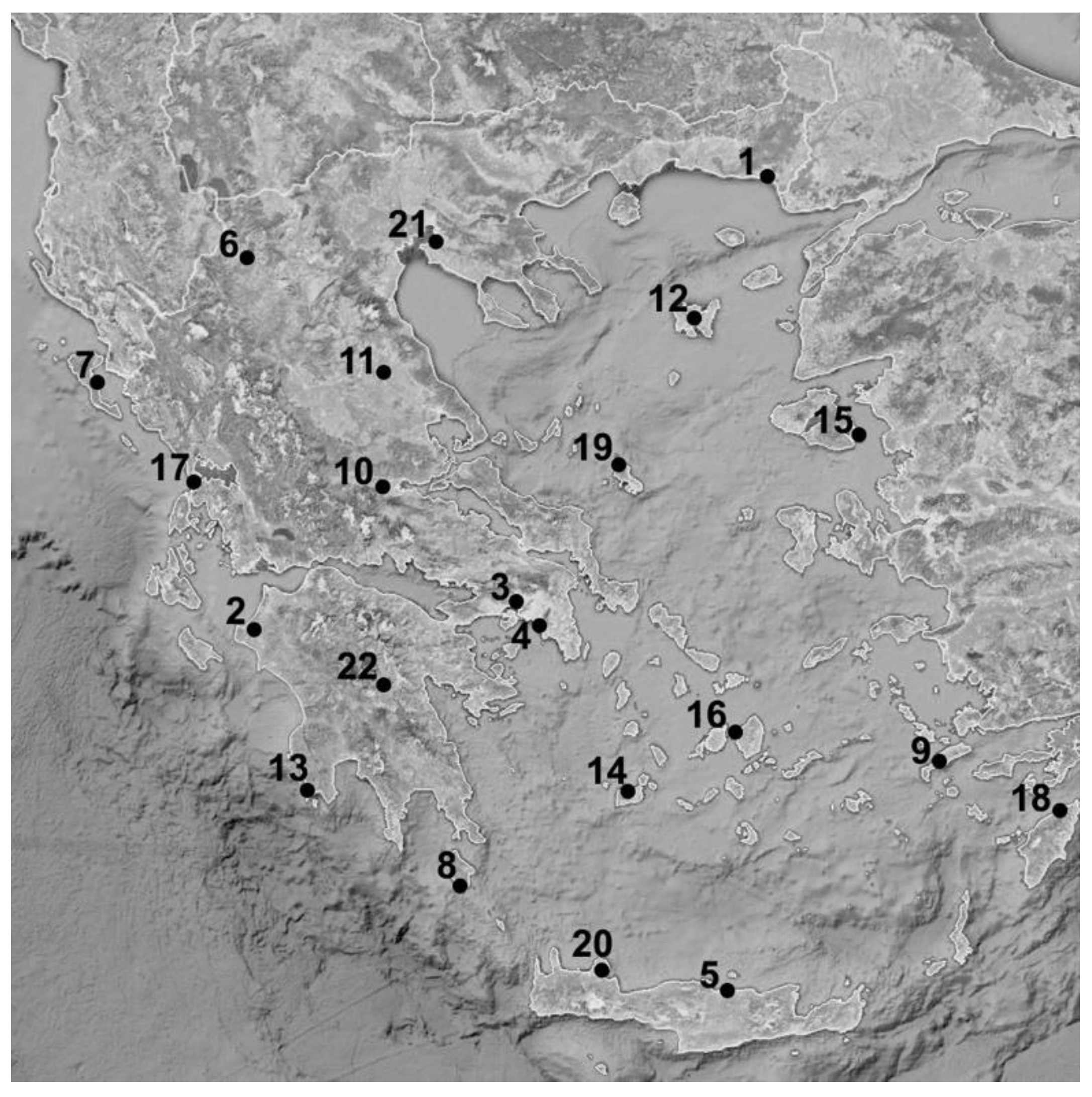
2.1. Experimental Data

In this study, we used data from 22 meteorological stations of the Hellenic National Meteorological Service (HNMS) network. These stations are listed in

Table 1. Meteorological stations and observation period.

No.	Station	Lat (°N)	Lon (°E)	Elevation (m)	Period	Completeness (%)
1	Alexandroupoli	40°51′27″	25°56′49″	3.52	1973–2014	99.64
2	Andravida	37°55′22″	21°17′15″	10.10	1973–2014	98.75
3	Elefsina	38°04′03″	23°33′08″	26.54	1973–2014	99.14
4	Hellinikon	37°53′23″	23°44′31″	43.13	1973–2012	98.51
5	Herakleion	35°20′07″	25°10′55″	39.00	1973–2014	99.93
6	Kastoria	40°26′56″	21°16′25″	654.64	1981–2014	97.18
7	Kerkira	39°36′29″	19°54′50″	1.13	1973–2014	99.94
8	Kithira	36°08′57″	22°59′19″	166.10	1973–2014	97.02
9	Kos	36°48′02″	27°05′29″	126.00	1983–2014	99.21
10	Lamia	38°52′35″	22°26′10″	12.46	1973–2014	96.19
11	Larisa	39°38′46″	22°27′37″	72.72	1973–2014	98.70
12	Limnos	39°55′22″	25°13′58″	1.90	1977–2014	99.40
13	Methoni	36°49′31″	21°42′16″	51.84	1973–2014	97.97
14	Milos	36°44′19″	24°25′45″	166.85	1973–2010	97.93
15	Mitilini	39°03′15″	26°36′14″	4.22	1973–2014	99.52
16	Naxos	37°06′05″	25°22′24″	9.00	1973–2014	97.24
17	Preveza	38°55′19″	20°46′08″	2.10	1973–2014	98.47
18	Rodos	36°24′08″	28°05′18″	6.63	1973–2014	99.93
19	Skiros	38°57′46″	24°29′27″	22.00	1973–2014	98.10
20	Souda	35°31′44″	24°08′43″	147.64	1973–2014	98.74
21	Thessaloniki	40°31′39″	22°58′18″	1.68	1973–2014	99.89
22	Tripoli	37°31′29″	22°23′50″	650.57	1973–2014	97.95

, while their spatial distribution is illustrated in Figure 1. The main criteria for the selection of these stations are: a) the length of the time series, b) the time series completeness (i.e., having very few missing values) and c) the spatial coverage (effort was made to cover all climatic and topographic areas of Greece).

The experimental data used in this study are the mean, maximum and minimum daily temperature time series (T_mean, T_max and T_min, respectively) at 2m above the ground level for the stations and the relevant periods listed in Table 1. The time series are extracted from the Global Summary Of the Day (GSOD) NOAA database [39]. In this database, quality assurance checks are performed regularly. In brief, a series of quality tests are applied to the dataset which can detect a variety of data problems, such as inconsistent climatological values with the location of the station, existence of unreal values, comparison with neighboring stations’ values and many others (more details can be found in [40]). Furthermore, a manual quality assurance check is performed to increase the reliability of the dataset. It should be noted that data completeness of all stations is above 95%. The level of data completeness is listed in Table 1. The few missing values are isolated and they are replaced using interpolation of their non-missing neighboring values. This very high data completeness is well over the minimum level of 50% at which the scaling exponent and therefore the scaling behavior of the time series are not seriously affected [41,42]. Therefore, MF-DFA can be reliably applied to the time series.

Additionally, daily data of wind speed, relative humidity, pressure and precipitation amount (for the same stations and periods) that are used later in this study have also been extracted from the same database.

2.2. Methodology

This study consists of the following steps:

• The multifractal characteristics of T_mean, T_max and T_min are studied for each station in terms of MF-DFA analysis.
• Assessment of the spatial distribution of the main multifractal spectrum characteristics is performed.
• Intercorrelations between multifractal spectrum parameters are examined.

MF-DFA analysis is applied to the temperature time series in order to examine their scaling properties. This method is described in detail by [26]. Herein, we give a brief description of the method.

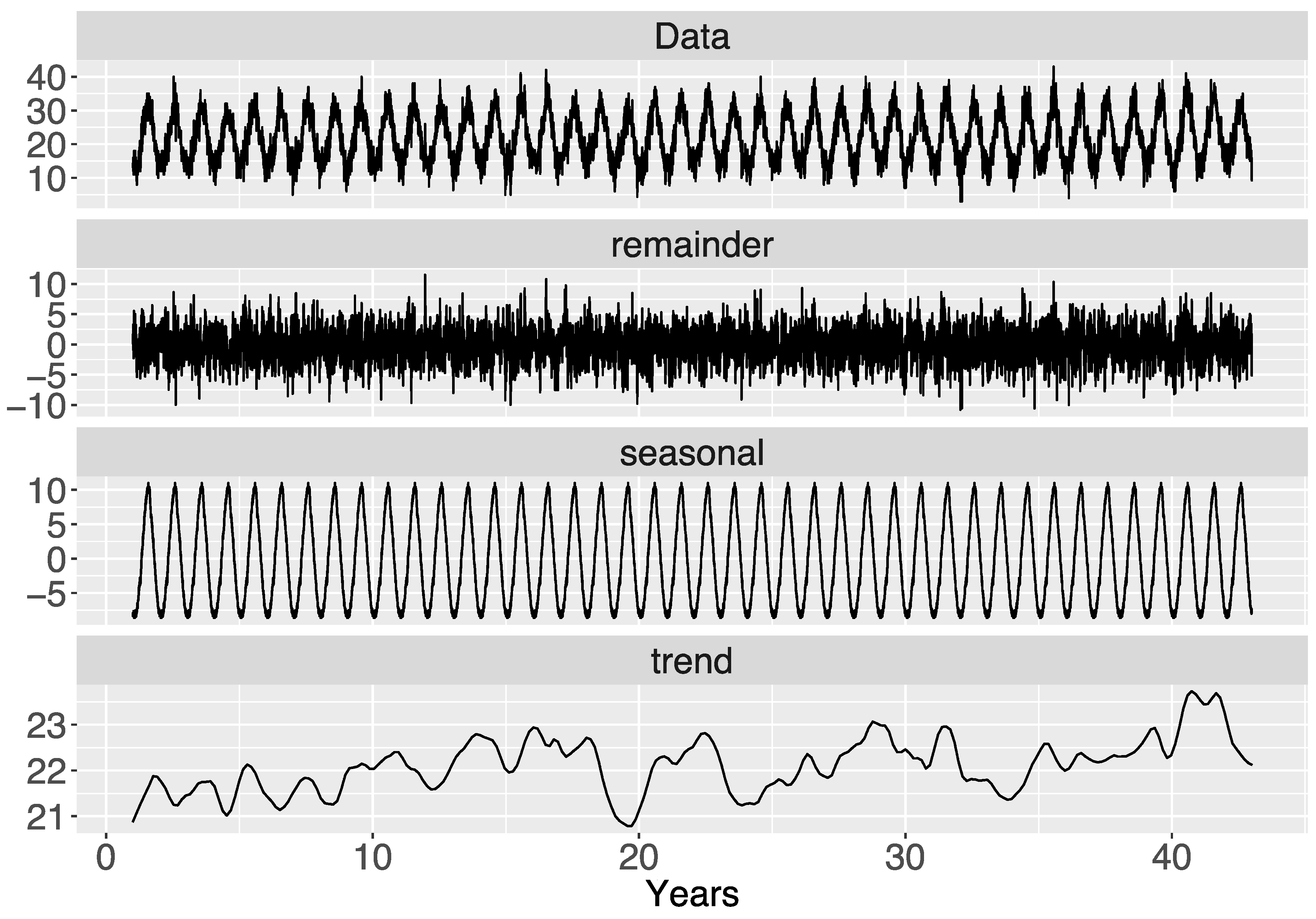
• First, the time series has to be deseasonalized. It is obvious that daily temperature time series exhibit periodical trends, which are attributed to the annual seasonal cycle. In general, periodical trends have an influence in the nonlinear properties of the time series [38] and therefore the time series should be deseasonalized before applying the MF-DFA method. An efficient method to deseasonalize a time series is the Seasonal and Trend decomposition using Loess (STL) method, which was introduced by [43]. In the STL method, the time series is decomposed into seasonal, trend and remainder components. From the decomposed time series, seasonality is removed and MF-DFA analysis is performed on the deseasonalized time series. A successful utilization of the STL method is presented by [44] with the aim to study the streamflow in the Yellow River basin, using MF-DFA.
• Then, we find the ‘profile’ Y(i) of the deseasonalized time series x_k of length N:

  $$Y(i)\equiv {\displaystyle \sum _{k=1}^i[x_k-<x>]}$$

  (1)

  where <x> is the mean of the time series and i = 1, …, N.
• Y(i) is then divided into N_s ≡ int(N/s) boxes of equal length s, where s is the ‘time scale’. It should be noted that N/s must be an integer, otherwise there will be a remaining number of profile points. However, very often N/s is not an integer and this problem is overcome by repeating the same procedure starting from the end. Thus, we get 2N_s boxes.
• In each box of length s, a least squares line is fitted to the data, which represents the trend in that box, i.e., the local trend. By subtracting the local trends, we detrend Y(i) and thus the variance F₂(ν,s) of each segment (box) ν (ν = 1, …, 2N_s) is calculated.
• Taking the average over all segments, we find the qth order fluctuation function:

  $$F_q(s)\equiv {\left\{\frac{1}{2N_s}{\displaystyle \sum _{v=1}^{2N_s}{[F^2(v,s)]}^{\frac{q}{2}}}\right\}}^{\frac{1}{q}}$$

  (2)
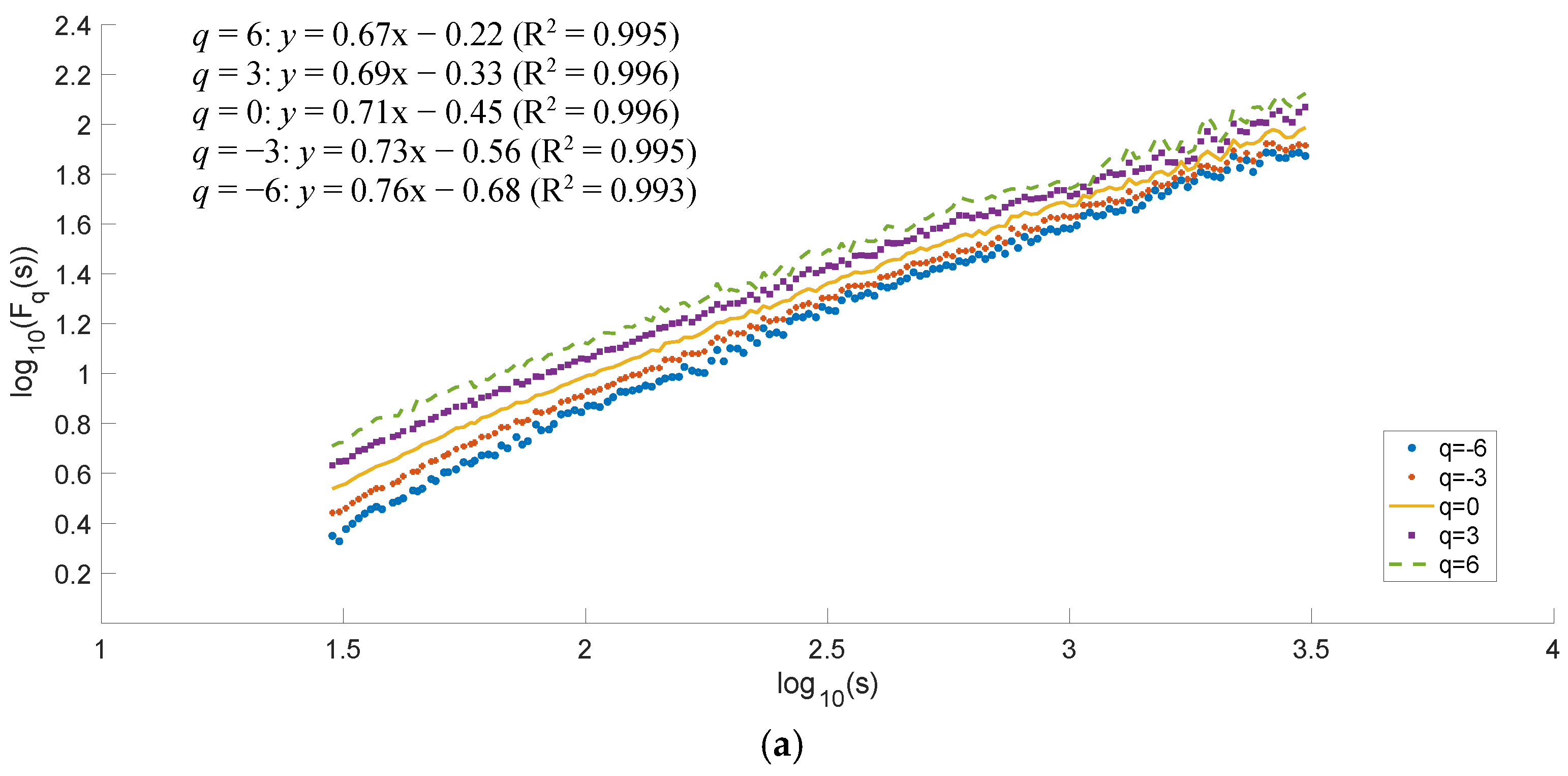
• This quantity is calculated repeatedly for all time scales to determine the relationship between F_q(s) and s. Typically F_q(s) is an increasing function of s.
• Making the log-log plots F_q(s) versus s for each value of q, we can examine the scaling behavior of F_q(s). If the series x_k are long-range power-law correlated, F_q(s) increases following a power-law:

  $$F_q(s)~s^{h(q)}$$

  (3)

The exponent h(q) usually depends on q. If q = 2, then, for stationary time series, h(2) is the Hurst exponent H. If the time series is monofractal, then h(q) is independent of q. In the case of different scaling between small and large fluctuations, significant dependencies are observed.

From (3), it is clear that h(q) takes a variety of values (for each value of q) for multifractal signals and it is called generalized Hurst exponent. Neglecting for a moment the dependency of Hurst exponent on q and assuming that h(q) = H it is important to note that:

• If 0 < H < 0.5 then the time series is long-range anticorrelated, that is, an increase in the value is more likely to be followed by a decrease (anti-persistent behavior) and vice versa.
• If H = 0.5 the time series is uncorrelated (white noise). In this case, the probability that an increase will be followed by an increase or decrease is equal.
• If H > 0.5 the time series is long range positively correlated, that is, an increase is more likely to be followed by an increase (persistent behavior) and vice versa.

If we use the relationship τ(q) = qh(q) − 1, then (via a Legendre transform) τ’(q) = α and

f(α) = qα − τ(q) = q [α − h(q)] + 1

(4)

The quantity α is called singularity strength (or Hölder exponent) and f(α) expresses the dimension of the subset of the time series that is characterized by α. The plot of α versus f(α) is called singularity spectrum, or multifractal spectrum. Usually, this plot has the shape of an upside-down parabola as in Figure 2. From the multifractal spectrum we can draw significant conclusions about the multifractality of a time series. The value of α where f(α) becomes maximum is when df(α)/dα = 0 and this happens for q = 0. Then, from (4) we find that f(α)_max = 1. This value of α corresponds to the most dominant scaling behavior [45] and it is the dominant Hurst exponent. Hereafter, this quantity will be denoted by α₀.

The second important property of the spectrum is its width (α_max − α_min), where α_max and α_min are the maximum and the minimum values of α, respectively, for which f(α) = 0 as it is depicted in Figure 2 and it is a measure of the multifractality of the time series. A spectrum with a broad width is indicative of a strong multifractality (i.e., it has a ‘fine’ structure). If the width becomes smaller, then the time series tends to be a monofractal one. The spectrum width of a pure monofractal time series is equal to zero. More details about the multifractal spectrum can be found in [46]. A measure of the width of the multifractal spectrum can be obtained by fitting a second-order equation to the curve of the spectrum around α₀ as recommended by [47]:

G (α) = A(α − α₀)² + Β(α − α₀) + C

(5)

Among the three constants A, B, C, the most important is B, which is an asymmetry parameter. When B = 0, the shape of the spectrum is symmetrical, whereas for positive B values, the spectrum is right-skewed and for negative left-skewed [48]. A right-skewed spectrum is related to relatively strongly weighted high fractal exponents, while a left-skewed spectrum is indicative of low fractal exponents (a more ‘regular’ time series). According to [46], a time series with a high value of α₀, broad width and right-skewed spectrum is considered to be more ‘complex’ than a time series with the opposite characteristics.

Furthermore, the shape of the multifractal spectra can be also characterized by its truncation type. Considering the range of the q values, the shape of the spectra can be symmetrical, left or right truncated. In our case, the truncation type is grouped into 4 categories, LL, L, S and R where:

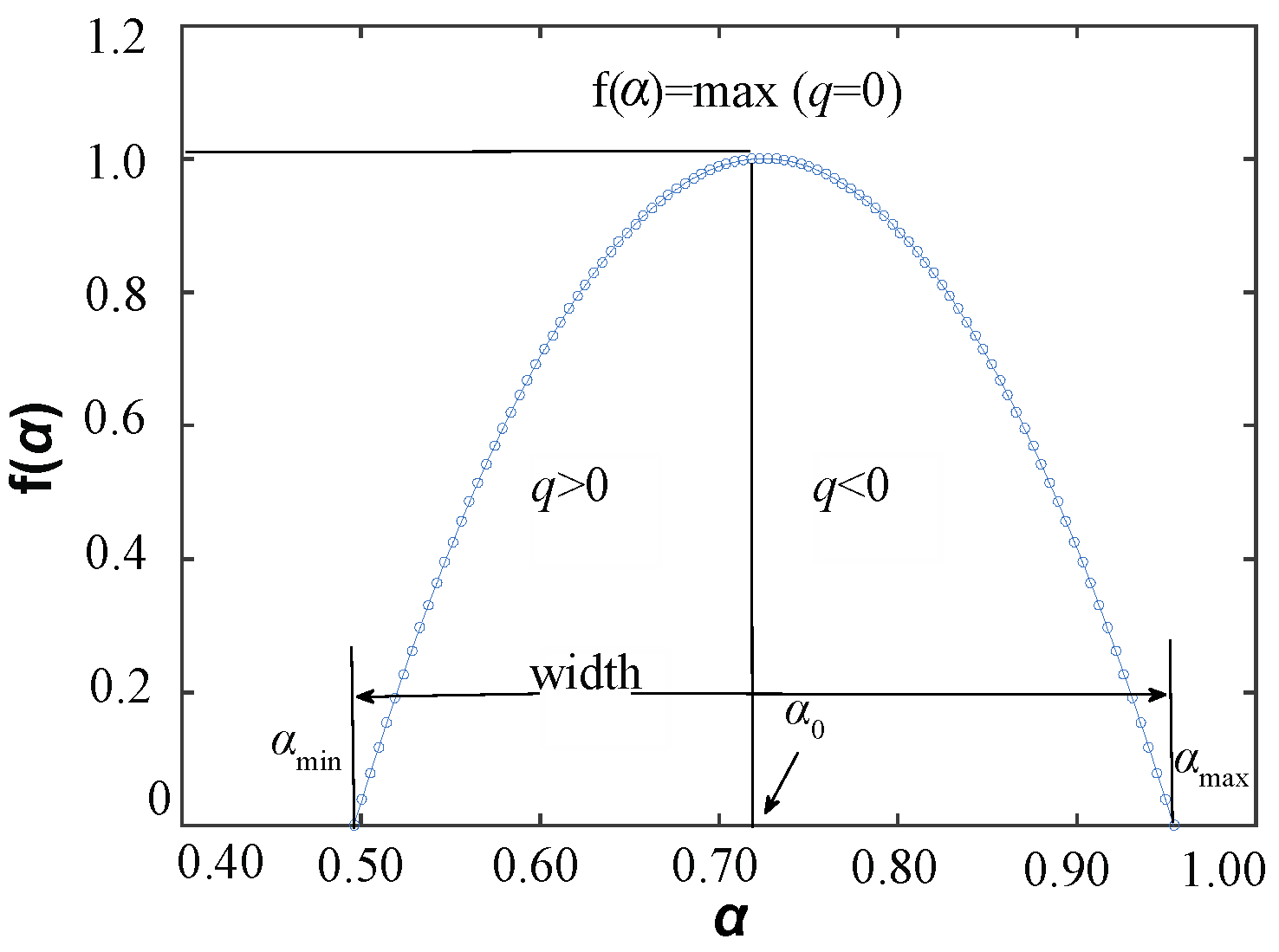
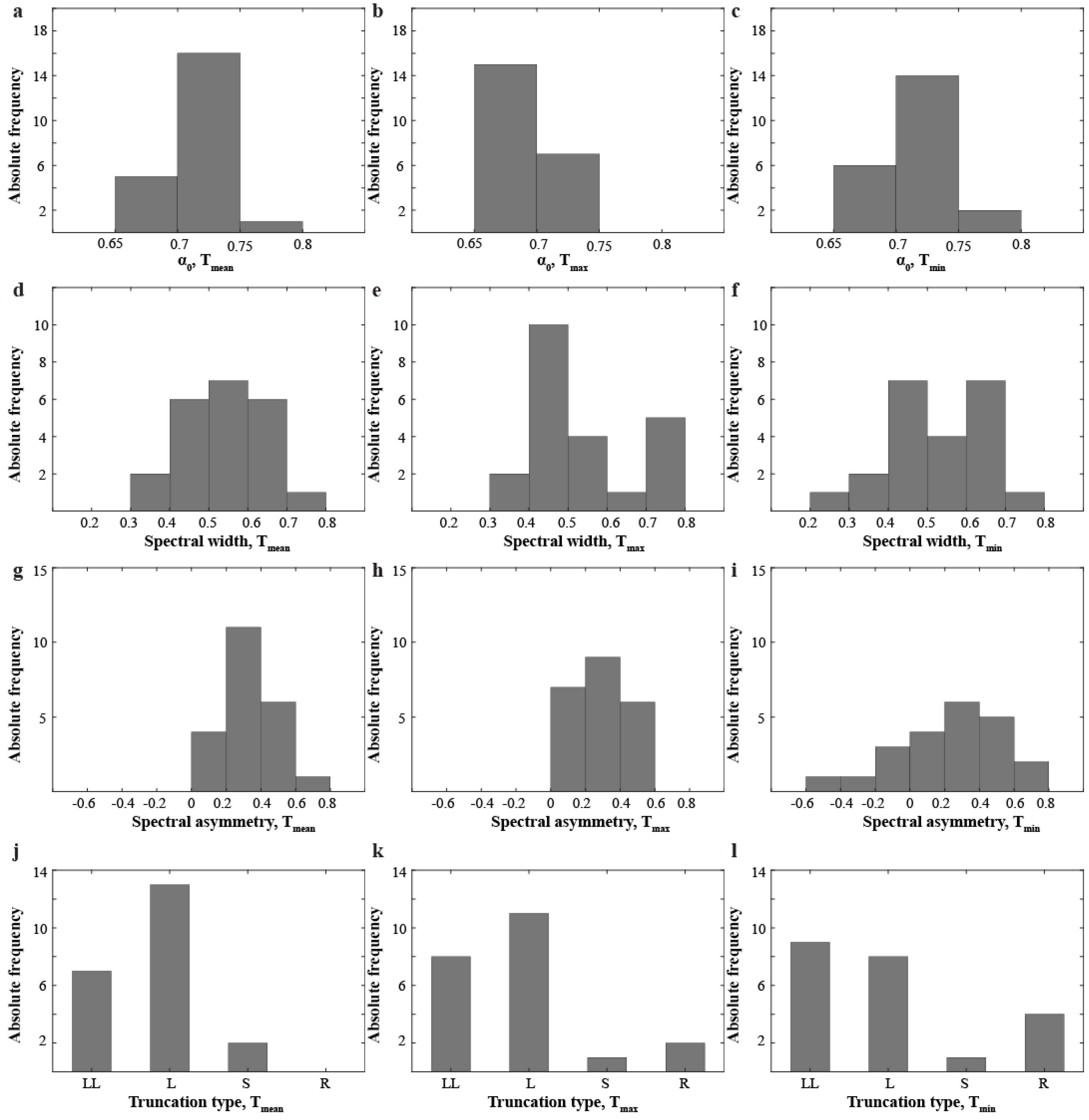
• L: the spectrum is left-truncated.
• LL: there is a high degree of truncation on the left side. (i.e., when the left leg of a spectrum is truncated more than its half-way point).
• R: the spectrum is right-truncated.
• S: the spectrum is symmetrical (there is no significant truncation).

To make this notation clearer, a representative plot for each case using experimental data is depicted in Figure 3. The left end of the curve of the spectrum corresponds to the greatest value of q (in our case q = 6) and the right end corresponds to the smallest q value (here q = −6), while the maximum value of f(α) corresponds to q = 0. Therefore, the spectrum is left-truncated then the change of f(α) is smaller for positive values of q than for negative ones, which means that the multifractal structure of the time series shows an insensitivity to local fluctuations with large magnitudes. Working in a similar way for the right-truncated spectrum, we find that there is insensitivity to local fluctuations with small magnitudes. If the spectrum is symmetrical, then the multifractal structure of the time series exhibits the same sensitivity regardless the magnitude of local fluctuations [45].

According to [27], multifractality is caused due to either a broad probability density function for the time series values or to different long-range correlations for fluctuations of large and small magnitudes. In order to examine which of the two cases causes multifractality in a time series, its values are ordered randomly (shuffled) and MF-DFA is applied to the shuffled time series. In the case where multifractal characteristics are preserved, then multifractality is caused by a broad probability density function. In the other case (i.e., the multifractality of the shuffled time series appears to be significantly weaker than that of the original time series), the multifractality is mainly due to different long-range correlations for different magnitudes of the time series fluctuations. However, in nature, multifractality can be driven by one of the sources or simultaneously by both of them [49,50].

Finally, the effects of seasonality and trends on the analyzed time series are subject to uncertainties regarding the DFA and therefore, MF-DFA results [41,51].

3. Results and Discussion

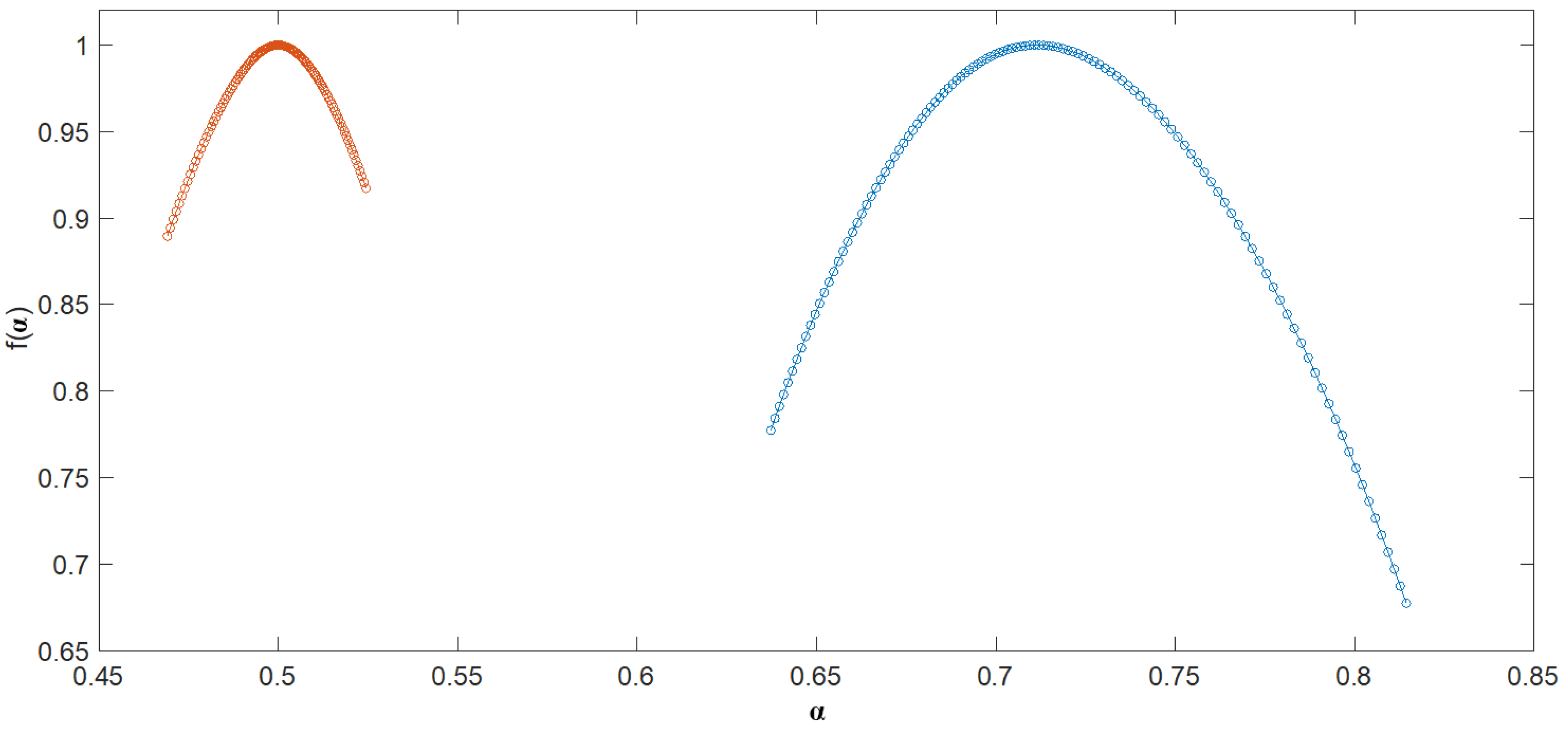
3.1. Air Temperature Multifractal Characteristics

Prior to MF-DFA analysis, the STL decomposition method is applied to the temperature time series. The resulting components along with the original time series are illustrated in Figure 4.

Upon removing the seasonal component, MF-DFA analysis is applied to the deseasonalized time series. The plots of: i) Fluctuation function F_q(s) versus the time scale s (log-log plots), ii) Generalized Hurst exponent h(q) versus q and iii) Multifractal spectrum f(α) versus α are obtained for each time series for q ranging from −6 up to +6. Due to space limitations, only selected characteristic plots are presented. In Figure 5, the plots of F_q(s) vs s, h(q) vs q and the multifractal spectrum f(α) vs α are illustrated for Kerkira station (the same shape of the relevant plots was found for almost all stations under study). The values of s used for the plotting of F_q(s) are approximately from 30 days (s ≈ 10^1.5) to 8.5 years (s ≈ 10^3.5). It should be noted that the upper limit of the time scale is N/5, where N is the time series length and for stations with different time series lengths (i.e., different observation periods), the upper limit changes accordingly.

From the F_q(s) vs s log-log plots for all temperature time series of all stations, it is observed that they have the form of an almost straight line (i.e., constant slope). It is noteworthy that slope values decrease when q has greater values, i.e., in Figure 5 the slope is 0.76 for q = −6, while for q = 6 the slope is 0.67. Moreover, the coefficient of determination (Pearson correlation coefficient) for all q values is higher than 0.98, which means that these scaling exponents are considered to be representative of the underlying scaling phenomenon [52].

It should be mentioned that, in the small segments (s small), it is easier to distinguish local periods with small fluctuations (q < 0) from periods with large fluctuations (q > 0). On the other hand, the large segments include periods of small and large fluctuations and thus the differences in magnitude are cancelled. Therefore, for large time scales, the behavior of F_q(s) is more similar to that of monofractal time series [46]. This can be noted in Figure 5a, where for large time scales the lines of F_q(s) are coming closer together. It can also be observed that the log-log fit of F_q(s) is not very good for small values of s and especially for q = −6. This could be attributed to the fact that the root mean square value is very sensitive to local fluctuations with small magnitudes (q < 0, the smaller the q, the higher the sensitivity), especially for small segments (which correspond to small s values). This is reflected in the existence of a long right tail at the multifractal spectrum, as it has previously been explained in methodology section.

Calculating the slope of F_q(s) for a multitude of q values, the values of generalized Hurst exponent h(q) are obtained. Here, h(q) is calculated for q values from −6 up to +6 in steps of 0.1 and therefore h(q) is found for 120 values of q. The multifractality of the time series can be concluded from the h(q) versus q plots. The dependency of the generalized Hurst exponent h(q) on q is evident from Figure 5b and this is a characteristic of multifractal time series, whereas in monofractal time series, the Hurst exponent is constant. Moreover, the fact that h(q) > 0.5 for all temperature time series leads to the conclusion that these time series exhibit long-range positive correlations. This means that an increase in temperature values is more likely to be followed by another increase. Furthermore, the slope of h(q) is greater for negative q (i.e., for small fluctuations) than for positive values of q (large fluctuations), which means that there is a higher degree of multifractality for the smaller fluctuations, in agreement with the aforementioned relevant conclusion from F_q(s) plots. As it was previously mentioned, the multifractal spectrum reveals significant properties about the multifractality of the time series. Therefore, we focused on its main characteristics, the value of α₀, the width α_max − α_min, the asymmetry parameter B and the truncation type of the spectrum. The results are presented in

Table 2. Values of the main multifractal characteristics.

Station	Singularity Spectrum Width αmax − αmin			Value of α for f(α) = max			Asymmetry Parameter B			Truncation Type
	Tmean	Tmax	Tmin	Tmean	Tmax	Tmin	Tmean	Tmax	Tmin	Tmean	Tmax	Tmin
1	0.545	0.473	0.539	0.685	0.678	0.692	0.180	0.213	0.048	L	L	L
2	0.664	0.591	0.639	0.720	0.728	0.742	0.496	0.227	0.349	L	R	LL
3	0.629	0.628	0.614	0.708	0.700	0.704	0.416	0.504	0.250	LL	LL	LL
4	0.659	0.715	0.644	0.719	0.703	0.717	0.399	0.315	−0.018	LL	LL	LL
5	0.458	0.471	0.286	0.712	0.683	0.689	0.375	0.466	−0.322	L	LL	R
6	0.479	0.481	0.432	0.713	0.662	0.737	0.038	0.091	−0.484	L	L	R
7	0.447	0.342	0.515	0.712	0.711	0.717	0.224	0.286	0.153	L	L	L
8	0.388	0.431	0.364	0.688	0.679	0.697	0.497	0.374	0.627	LL	L	L
9	0.511	0.438	0.602	0.747	0.723	0.761	0.037	0.144	0.039	S	L	S
10	0.500	0.547	0.476	0.718	0.670	0.716	0.478	0.423	0.490	L	L	LL
11	0.659	0.717	0.666	0.684	0.699	0.734	0.685	0.569	0.420	LL	LL	LL
12	0.566	0.527	0.475	0.725	0.695	0.692	0.255	0.257	0.158	L	L	L
13	0.548	0.589	0.508	0.734	0.713	0.680	0.396	0.525	0.357	L	LL	L
14	0.470	0.439	0.492	0.696	0.682	0.709	0.214	0.215	0.226	L	L	L
15	0.532	0.446	0.537	0.715	0.678	0.715	0.269	0.074	0.301	L	S	LL
16	0.677	0.734	0.672	0.775	0.711	0.748	0.305	0.183	0.402	LL	LL	LL
17	0.727	0.759	0.716	0.720	0.700	0.728	0.577	0.493	0.522	LL	LL	LL
18	0.437	0.435	0.395	0.730	0.706	0.760	0.097	0.183	0.669	S	L	L
19	0.544	0.489	0.402	0.703	0.679	0.699	0.409	0.369	0.409	L	L	L
20	0.688	0.720	0.693	0.691	0.686	0.705	0.287	0.194	0.236	LL	LL	LL
21	0.463	0.431	0.496	0.717	0.693	0.721	0.299	0.345	−0.109	L	L	R
22	0.380	0.349	0.436	0.734	0.689	0.713	0.317	0.162	−0.068	L	R	R

.

Regarding the α₀ results, it is observed that the values are within a narrow zone ranging from 0.662 up to 0.775 for all time series. Thus, the dominant Hurst exponent of the examined temperature time series is of the order of 0.7, which means that the temperature time series are long range positively correlated. It should also be noted that for T_max the majority of α₀ values is between 0.65 and 0.70, while for T_mean and T_min the more α₀ values are in the range 0.70–0.75. Regarding the multifractal (singularity) spectrum width values, (Table 2) it is observed that there is a significant variation, ranging from 0.342 to 0.759 for T_max, from 0.380 to 0.727 for T_mean and from 0.286 to 0.716 for T_min and their distributions are illustrated in the histograms of Figure 6. It is observed that for all temperature time series (T_mean, T_max and T_min), the majority of the spectrum width values are within 0.4 and 0.7. The asymmetry parameter B values are in the range from −0.484 up to 0.685. It is easily noticeable that the majority of the B values are positive and that negative values are observed only for T_min. Thus, most of the spectra are right-skewed, which indicates that, in most cases, there are relatively strongly weighted high fractal exponents. Focusing on the truncation type, it is clear that the majority of the spectra are left-truncated, leading to the conclusion that, in general, the multifractal structure of temperature time series is robust to local fluctuations with large magnitudes.

Concerning the type of multifractality, MF-DFA application to the shuffled time series reveals that in all cases the multifractality is very weak and it is mainly due to different long-range correlations for small and large fluctuations. A characteristic case is presented in Figure 7, where the multifractal spectrum for Kerkira daily maximum temperature is depicted for both the original and the shuffled time series. It was found that in all temperature time series, the spectra for the original and shuffled time series are similar to those of Figure 7. In shuffled time series we observe that the width of the spectrum for the shuffled time series is much smaller than the original time series and the value of α₀ is very close to 0.5 and, therefore, diminished multifractality (compared to the unshuffled series) shows that long-range correlations play the main role in the multifractality of the data [26].

It should be noted that in order to avoid statistical errors, data shuffling of each time series was repeated 100 times, where the initial data from the time series were randomly shuffled at each repetition, and the mean values of multifractal parameters were calculated [49]. The corresponding mean value of the spectrum width for all stations and temperature time series is of the order of 0.2, i.e., in our case a time series with spectrum width less than 0.2 can be considered as monofractal [53]. Considering the values of spectrum width (Table 2), it is concluded that all temperature time series exhibit a multifractal behavior.

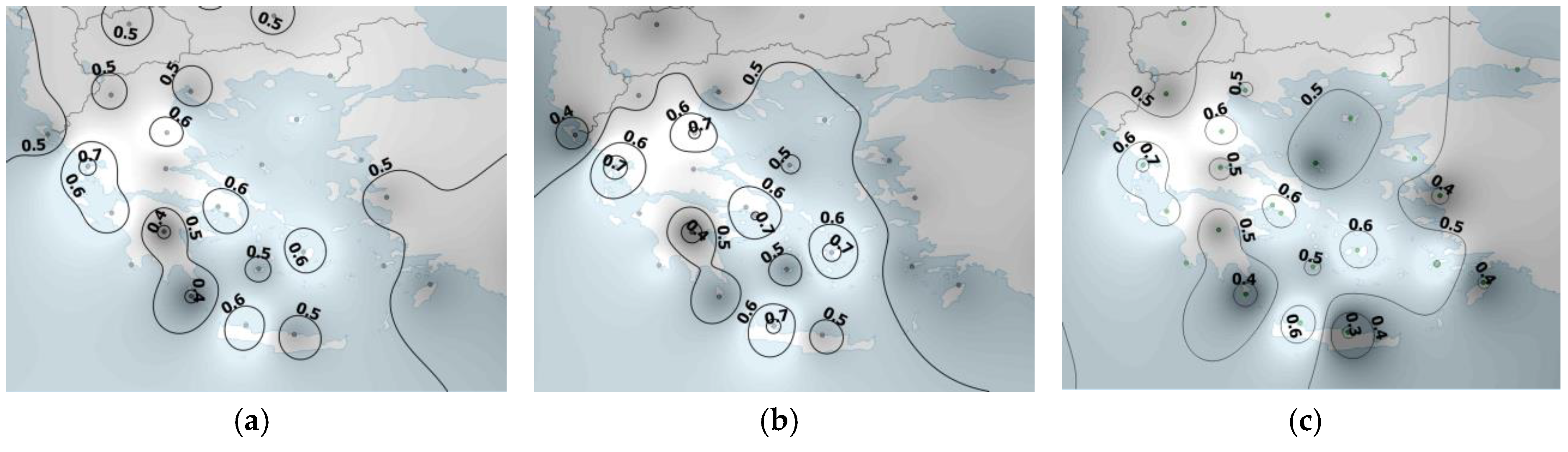
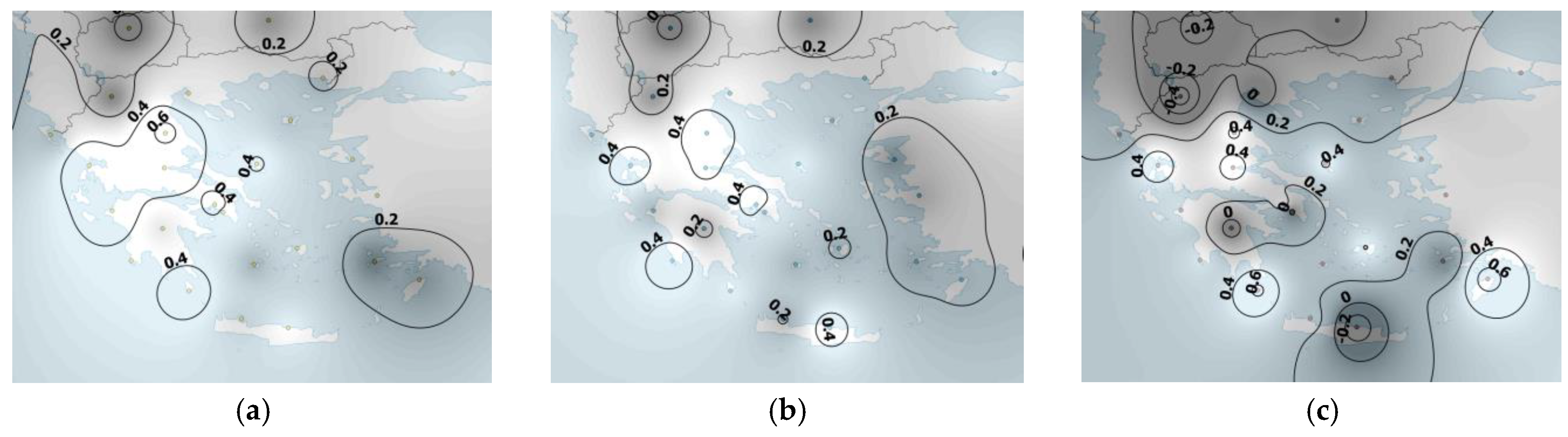
3.2. Spatial Distributions

The spatial distributions of spectral width, a₀ and asymetry parameter for the T_mean, T_max and T_min over Greece are illustrated in Figure 8, Figure 9 and Figure 10, respectively. For a better interpretation of those figures, isolines are also shown.

Regarding the spatial distribution of spectral width, two distinct regions are observed. A region of relatively higher multifractal spectrum width values, which includes a great part of continental Greece and Aegean Sea and a part of Ionian islands, and a region with lower spectrum values, which includes southeastern areas, a part of south mainland and parts of northwestern Greece. The first region has a richer multifractal spectrum, which means that weather conditions—and consequently the temperature—in this region are affected in a more ‘complex’ way than the rest of Greece. Possible causes of local day-to-day temperature variations are the depression tracks over Greece from western directions [54]. The first region includes the coastal areas of eastern mainland and some parts of the western Greece. Taking also into account the topography of Greece, temperature at these areas could be affected by other factors, such as cold outbreaks in the winter mainly in eastern Greece [55], the onset of Etesians winds in the summer mainly over Aegean Sea [56], katabatic winds causing Föhn effect, thermal instability in summer at continental areas, or probably other local circulations. On the other hand, the more ‘stable’ climatic conditions at the marine and coastal parts of the second region and the less irregular topography contribute towards a relatively simpler temperature variability.

The spatial distribution of α₀ values (Figure 9) exhibits a rather smooth field of the order of 0.7 (α₀ values are in the range 0.66–0.77 in the Greek area). Therefore, the prevailing behavior of all temperature time series is persistent, which means that an increase in temperature is more likely to be followed by another increase, in agreement with the values of h(q), as in Figure 5b. In more detail, relatively larger values are noticed at two geographical areas: i) At southeastern Greece and ii) At some parts of coastal western Greece. Considering that α₀ is the dominant Hurst exponent, it is deduced that temperature time series for these areas appear to have relatively more persistent behavior than the other areas of Greece. A possible explanation could be that these areas have more ‘stable’ climatic conditions throughout the year, which agrees with [14] results for Turkey. Additionally, the absence of rainfall in the summer period is more pronounced at coastal and marine areas, whereas in continental Greece, the precipitation amount exhibits a more uniform interannual distribution, due to atmospheric instability especially in the warm period [57,58]. Furthermore, it is also interesting that continental areas in Greece appear to have greater temperature variability than the marine and coastal areas [59] which is in partial agreement with the α₀ spatial distribution findings. It is noteworthy that higher α₀ values for the T_min time series—compared to the corresponding values for T_max and T_mean—are observed for a significant part of continental Greece. This could be attributed to the fact that summer thermal instability is observed at noon and in the afternoon whereas the minimum temperature is observed in the early morning.

Regarding the spectral asymmetry spatial distribution, it is observed that the lower values of parameter B are found, in general, mainly in southeastern Greece. Spectra with higher B values contain a greater number of high fractal components and therefore, according to [47,48] are related to more ‘complex’ time series and it could be assumed that the pre-mentioned greater climate stability at the southeastern area leads to less ‘complex’ time series.

Finally, it is noteworthy to mention that in order to achieve a coverage of the entire Greek area for the spatial distribution of the main multifractal characteristics, we used the relevant temperature data from 13 neighboring stations. These stations together with their main multifractal spectrum characteristics (which were found using the same analysis as for the Greek stations) are listed in

Table 3. Values of the main multifractal characteristics for neighboring stations.

Station	Singularity Spectrum Width αmax − αmin			Value of α for f(α) = max			Asymmetry Parameter B			Truncation Type
	Tmean	Tmax	Tmin	Tmean	Tmax	Tmin	Tmean	Tmax	Tmin	Tmean	Tmax	Tmin
23	0.491	0.584	0.387	0.791	0.728	0.731	0.339	0.320	0.565	L	L	LL
24	0.577	0.542	0.517	0.697	0.668	0.713	0.294	0.306	0.298	L	LL	L
25	0.494	0.449	0.516	0.693	0.670	0.694	0.255	0.325	−0.082	L	L	S
26	0.488	0.487	0.511	0.683	0.694	0.676	0.068	0.043	−0.106	L	L	S
27	0.426	0.499	0.311	0.751	0.749	0.733	0.720	0.450	0.704	L	L	L
28	0.409	0.334	0.195	0.742	0.722	0.750	−0.022	0.455	−0.328	R	L	L
29	0.458	0.405	0.459	0.743	0.752	0.731	0.121	0.410	0.312	L	L	L
30	0.367	0.541	0.312	0.776	0.753	0.765	0.165	0.600	1.046	L	L	S
31	0.408	0.452	0.373	0.759	0.751	0.721	−0.098	−0.233	0.114	S	R	L
32	0.392	0.397	0.445	0.700	0.653	0.751	0.139	0.125	0.180	L	L	L
33	0.506	0.431	0.463	0.716	0.689	0.743	0.337	0.341	0.294	L	L	L
34	0.459	0.448	0.385	0.703	0.677	0.684	0.262	0.099	0.270	L	S	L
35	0.489	0.418	0.487	0.707	0.688	0.710	−0.058	−0.052	−0.275	S	S	R

Stations: 23: Alexandria, 24: Benghazi, 25: Sofia, 26: Plovdiv, 27: Pafos, 28: Brindisi, 29: S.M. Leuca, 30: R. Calabria, 31: Malta, 32: Antalya, 33: Istanbul, 34: Izmir, 35: Skopje.

. A brief remark about the stations of Table 3 is that the values of the singularity spectrum width are in the same ranges as the Greek stations.

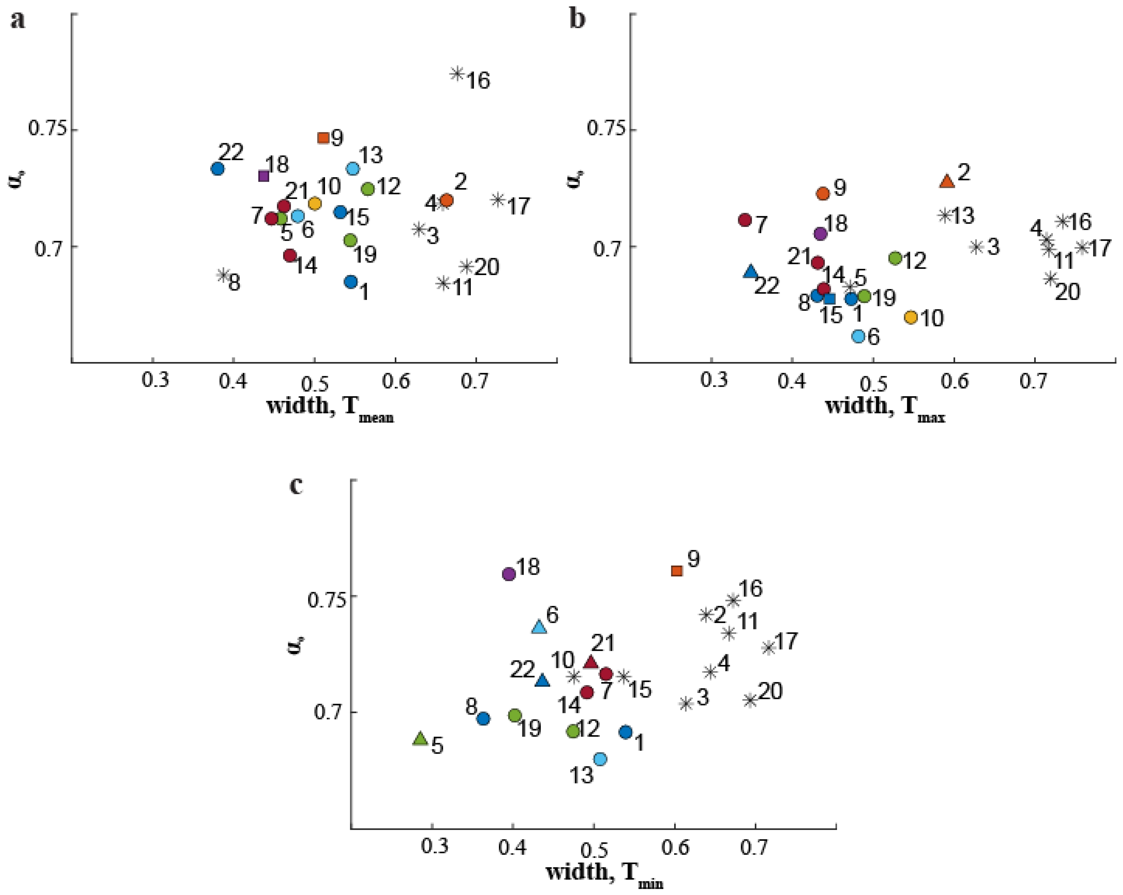
3.3. Multifractal Spectrum Parameters Intercorrelations

Regarding the multifractal spectrum parameter intercorrelations, we examined initially the relationship of a₀ and width with B and subsequently their relationship with the truncation type. Although no clear relationship was found between α₀ and spectral width, the analysis revealed a well-defined group of stations with LL truncation type, for α₀ > 0.68 and spectral width >0.6 for all temperature time series (T_mean, T_max and T_min) as illustrated in Figure 11. These cases, considering that a left truncated spectrum has mainly high fractal exponents (i.e., ‘fine’ structure), can be considered more complex than the remaining time series. It should also be noted that no significant geographical correlations were revealed; a similar finding was found in another Mediterranean region [48].

Finally, we examined the correlation between the multifractal parameters of temperature time series and the main descriptive statistical parameters (i.e., mean, standard deviation, skewness and kurtosis) of the main climatic parameters (i.e., relative humidity, wind speed and precipitation amount). The results did not exhibit a clear association, verifying the complexity of the factors that affect temperature fluctuations.

4. Conclusions

The analysis reveals that air temperature over the study area exhibits long-range temporal correlations that cannot be fully described by a single scaling exponent. According to the F_q(s) vs. s plots, the multifractal character of the examined temperature time series is verified for all sites. The generalized Hurst exponent h(q) is dependent on q in all cases, thus confirming the multifractal nature of the examined time series. It is also found that h(q) is greater than 0.5, which reveals that the time series are long-term positive correlated, meaning that an increase in temperature is more likely to be followed by another increase. Emphasizing the multifractal spectrum (i.e., f(α) vs. α plots), significant multifractal features were deduced from examining the dominant Hurst exponent (α₀), the spectrum width, the asymmetry parameter B and the truncation type. The spatial distribution of the above parameters indicates that larger multifractal spectrum widths could be associated with regions where weather conditions and consequently the temperature are affected in a more ‘complex’ way than in other areas. Furthermore, relatively higher α₀ values as well as higher values of the parameter B may be associated with regions of more stable climatic conditions. The dominant truncation type is left truncation, and thus for the vast majority of the time series, their multifractal structure is insensitive to larger local variations of temperature. In general, atmospheric circulation and weather conditions affect the shape of the spectrum, and the corresponding spatial distributions results highlight the complexity with which the natural processes interact and the importance of finding associations among the multifractal characteristics and different atmospheric processes. Moreover, the intercorrelation results among α₀ and spectrum width with the truncation type revealed a well-defined group of stations that exhibit similar multifractal characteristics. In particular, left truncation spectra are, in general, associated with higher spectrum width values. In addition, the analysis presented in this study could be useful for assessing the performance of climate models in terms of their ability to simulate reasonably well the observed air temperature non-linear dynamics. More specifically, as future work, the proposed methodology will be performed at larger or even global spatial scales for experimental temperature datasets and climate model simulations.

References

1. Pielke, R.A. Mesoscale Meteorological Modelling; Academic Press Inc: Orlando, FL, USA, 1984. [Google Scholar]
2. Kantz, H.; Schreiber, T. Nonlinear Time Series Analysis, 2nd ed.; Cambridge University Press: Cambridge, UK, 2004. [Google Scholar]
3. Peng, C.K.; Buldyrev, S.V.; Havlin, S.; Simons, M.; Stanley, H.E.; Goldberger, A.L. Mosaic organization of DNA nucleotides. Phys. Rev. E 1994, 49, 1685–1689. [Google Scholar] [CrossRef]
4. Kantelhardt, J.W.; Koscielny-Bunde, E.; Rego, H.H.A.; Havlin, S.; Bunde, A. Detecting long-range correlations with detrended fluctuation analysis. Physica A 2001, 295, 441–454. [Google Scholar] [CrossRef] [Green Version]
5. Liu, Y.; Cizeau, P.; Meyer, M.; Peng, C.K.; Stanley, H.E. Correlations in economic time series. Physica A 1997, 245, 437–440. [Google Scholar] [CrossRef] [Green Version]
6. Di Matteo, T.; Aste, T.; Dacorogna, M.M. Scaling behaviors in differently developed markets. Physica A 2003, 324, 183–188. [Google Scholar] [CrossRef]
7. Barbi, M.; Chillemi, S.; Di Garbo, A.; Balocchi, R.; Carpeggiani, C.; Emdin, M.; Michelassi, C.; Santarcangelo, E. Predictability and nonlinearity of the heart rhythm. Chaos Soliton Fractals 1998, 9, 507–515. [Google Scholar] [CrossRef]
8. Buldyrev, S.V.; Dokholyan, N.V.; Goldberger, A.L.; Havlin, S.; Peng, C.K.; Stanley, H.E.; Viswanathan, G.M. Analysis of DNA sequences using methods of statistical physics. Physica A 1998, 249, 430–438. [Google Scholar] [CrossRef] [Green Version]
9. Gao, J.; Hu, J.; Mao, X.; Perc, M. Culturomics meets random fractal theory: Insights into long-range correlations of social and natural phenomena over the past two centuries. J. R. Soc. Interface 2012, 9, 1956–1964. [Google Scholar] [CrossRef] [PubMed]
10. Varotsos, C.A.; Melnikova, I.; Efstathiou, M.N.; Tzanis, C. 1/f noise in the UV solar spectral irradiance. Theor. Appl. Climatol. 2013, 111, 641–648. [Google Scholar] [CrossRef]
11. Chattopadhyay, G.; Chattopadhyay, S. Study on statistical aspects of monthly sunspot number time series and its long-range correlation through detrended fluctuation analysis. Indian J. Phys. 2014, 88, 1135–1140. [Google Scholar] [CrossRef]
12. Eichner, J.F.; Koscielny-Bunde, E.; Bunde, A.; Havlin, S.; Schellnhuber, H.J. Power-law persistence and trends in the atmosphere: A detailed study of long temperature records. Phys. Rev. E 2003, 68, 046133. [Google Scholar] [CrossRef] [PubMed] [Green Version]
13. Bartos, I.; Janosi, I.M. Nonlinear correlations of daily temperature records over land. Nonlinear Process. Geophys. 2006, 13, 571–576. [Google Scholar] [CrossRef] [Green Version]
14. Orun, M.; Koçak, K. Application of detrended fluctuation analysis to temperature data from Turkey. Int. J. Clim. 2009, 29, 2130–2136. [Google Scholar] [CrossRef]
15. Yuan, N.; Fu, Z.; Mao, J. Different scaling behaviors in daily temperature records over China. Physica A 2010, 389, 4087–4095. [Google Scholar] [CrossRef]
16. Kalamaras, N.; Philipppopoulos, K.; Deligiorgi, D. Scaling Properties of Meteorological Time Series Using Detrended Fluctuation Analysis. In Perspectives on Atmospheric Sciences, Proceedings of the 13th International Conference of Meteorology, Climatology and Atmospheric Physics, Thessaloniki, Greece, 19–21 September 2016; Karacostas, T.S., Bais, A.F., Nastos, P.T., Eds.; Springer Atmospheric Physics; Springer: Cham, Switzerland, 2016; pp. 545–550. [Google Scholar]
17. Podobnik, B.; Ivanov, P.C.; Jazbinsek, V.; Trontelj, Z.; Stanley, H.E.; Grosse, I. Power-law correlated processes with asymmetric distributions. Phys. Rev. E 2005, 71, 025104. [Google Scholar] [CrossRef] [PubMed]
18. Lin, G.; Chen, X.; Fu, Z. Temporal–spatial diversities of long-range correlation for relative humidity over China. Physica A 2007, 383, 585–594. [Google Scholar] [CrossRef]
19. Jiang, L.; Li, N.; Zhao, X. Scaling behaviors of precipitation over China. Theor. Appl. Climatol. 2017, 128, 63–70. [Google Scholar] [CrossRef]
20. He, W.; Zhao, S.; Liu, Q.; Jiang, Y.; Deng, B. Long-range correlation in the drought and flood index from 1470 to 2000 in eastern China. Int. J. Clim. 2016, 36, 1676–1685. [Google Scholar] [CrossRef]
21. Varotsos, C.A.; Tzanis, C. A new tool for the study of the ozone hole dynamics over Antarctica. Atmos. Environ. 2012, 47, 428–434. [Google Scholar] [CrossRef]
22. Varotsos, C.A.; Milinevsky, G.; Grytsai, A.; Efstathiou, M.; Tzanis, C. Scaling effect in planetary waves over Antarctica. Int. J. Remote Sens. 2008, 29, 2697–2704. [Google Scholar] [CrossRef]
23. Varotsos, C.; Efstathiou, M.; Tzanis, C.; Deligiorgi, D. On the limits of the air pollution predictability: The case of the surface ozone at Athens, Greece. Environ. Sci. Pollut. Res. 2012, 19, 295–300. [Google Scholar] [CrossRef]
24. Varotsos, C.; Tzanis, C.; Efstathiou, M.; Deligiorgi, D. Tempting long-memory in the historic surface ozone concentrations at Athens, Greece. Atmos. Pollut. Res. 2015, 6, 1055–1057. [Google Scholar] [CrossRef]
25. Horvatic, D.; Stanley, H.E.; Podobnik, B. Detrended cross-correlation analysis for non-stationary time series with periodic trends. Europhys. Lett. 2011, 94, 18007. [Google Scholar] [CrossRef]
26. Kantelhardt, J.W.; Zschiegner, S.A.; Koscielny-Bunde, E.; Havlin, S.; Bunde, A.; Stanley, H.E. Multifractal detrended fluctuation analysis of nonstationary time series. Physica A 2002, 316, 87–114. [Google Scholar] [CrossRef] [Green Version]
27. Kalamaras, N.; Philippopoulos, K.; Deligiorgi, D.; Tzanis, C.G.; Karvounis, G. Multifractal scaling properties of daily air temperature time series. Chaos Soliton Fractals 2017, 98, 38–43. [Google Scholar] [CrossRef]
28. Svensson, C.; Olsson, J.; Berndtsson, R. Multifractal properties of daily rainfall in two different climates. Water Resour. Res. 1996, 332, 2463–2472. [Google Scholar] [CrossRef]
29. Du, H.; Wu, Z.; Zong, S.; Meng, X.; Wang, L. Assessing the characteristics of extreme precipitation over northeast China using the multifractal detrended fluctuation analysis. J. Geophys. Res. Atmos. 2013, 118, 6165–6174. [Google Scholar] [CrossRef] [Green Version]
30. Kavasseri, R.G.; Nagarajan, R. A multifractal description of wind speed records. Chaos Soliton Fractals 2005, 24, 165–173. [Google Scholar] [CrossRef] [Green Version]
31. Feng, T.; Fu, Z.; Deng, X.; Mao, J. A brief description to different multi-fractal behaviors of daily wind speed records over China. Phys. Lett. A 2009, 373, 4134–4141. [Google Scholar] [CrossRef]
32. Pedron, I.T. Correlation and multifractality in climatological time series. J. Phys. Conf. Ser. 2010, 246, 012034. [Google Scholar] [CrossRef] [Green Version]
33. Baranowski, P.; Krzyszczak, J.; Slawinski, C.; Hoffmann, H.; Kozyra, J.; Nieróbca, A.; Siwek, K.; Gluza, A. Multifractal analysis of meteorological time series to assess climate impacts. Clim. Res. 2015, 65, 39–52. [Google Scholar] [CrossRef]
34. Xue, Y.; Pan, W.; Lu, W.; He, H. Multifractal nature of particulate matters (PMs) in Hong Kong urban air. Sci. Total Environ. 2015, 532, 744–751. [Google Scholar] [CrossRef] [PubMed]
35. Movahed, M.S.; Jafari, G.R.; Ghasemi, F.; Rahvar, S.; Tabar, M.R.R. Multifractal detrended fluctuation analysis of sunspot time series. J. Stat. Mech. Theory Exp. 2006, 2, P02003. [Google Scholar] [CrossRef]
36. Laib, M.; Telesca, L.; Kanevski, M. Long-range fluctuations and multifractality in connectivity density time series of a wind speed monitoring network. Chaos 2018, 28, 033108. [Google Scholar] [CrossRef] [PubMed] [Green Version]
37. Hoffmann, H.; Baranowski, P.; Krzyszczak, J.; Zubik, M.; Sławiński, C.; Gaiser, T.; Ewert, F. Temporal properties of spatially aggregated meteorological time series. Agric. For. Meteorol. 2017, 234–235, 247–257. [Google Scholar] [CrossRef]
38. Krzyszczak, J.; Baranowski, P.; Zubik, M.; Hoffmann, H. Temporal scale influence on multifractal properties of agro-meteorological time series. Agric. For. Meteorol. 2017, 239, 223–235. [Google Scholar] [CrossRef]
39. Menne, M.J.; Durre, I.; Vose, R.S.; Gleason, B.E.; Houston, T.G. An Overview of the Global Historical Climatology Network-Daily Database. J. Atmos. Ocean. Technol. 2012, 29, 897–910. [Google Scholar] [CrossRef]
40. Durre, I.; Menne, M.J.; Gleason, B.E.; Houston, T.G.; Vose, R.S. Comprehensive Automated Quality Assurance of Daily Surface Observations. J. Appl. Meteorol. Clim. 2010, 49, 1615–1633. [Google Scholar] [CrossRef]
41. Chen, Z.; Ivanov, P.C.; Hu, K.; Stanley, H.E. Effect of nonstationarities on detrended fluctuation analysis. Phys. Rev. E 2002, 65, 041107. [Google Scholar] [CrossRef]
42. Mirzayof, D.; Ashkenazy, Y. Preservation of long range temporal correlations under extreme random dilution. Physica A 2010, 389, 5573–5580. [Google Scholar] [CrossRef]
43. Cleveland, R.B.; Cleveland, W.S.; McRae, J.E.; Terpenning, I. STL: A Seasonal-Trend Decomposition Procedure Based on Loess. J. Off. Stat. 1990, 6, 3–33. [Google Scholar]
44. Li, E.; Mu, X.; Zhao, G.; Gao, P. Multifractal Detrended Fluctuation Analysis of Streamflow in the Yellow River Basin, China. Water 2015, 7, 1670–1686. [Google Scholar] [CrossRef] [Green Version]
45. Bishop, S.M.; Yarham, S.I.; Navapurkar, V.U.; Menon, D.K.; Ercole, A. Multifractal analysis of hemodynamic behavior: Intraoperative instability and its pharmacological manipulation. Anesthesiology 2012, 117, 810–821. [Google Scholar] [CrossRef] [PubMed]
46. Ihlen, E.A.F. Introduction to multifractal detrended fluctuation analysis in Matlab. Front. Physiol. 2012, 3, 141. [Google Scholar] [CrossRef] [PubMed]
47. Shimizu, Y.; Thurner, K.; Ehrenberger, K. Multifractal spectra as a measure of complexity in human posture. Fractals 2002, 10, 103–116. [Google Scholar] [CrossRef]
48. Burgueno, A.; Lana, X.; Serra, C.; Martinez, M.D. Daily extreme temperature multifractals in Catalonia (NE Spain). Phys. Lett. A 2014, 378, 874–885. [Google Scholar] [CrossRef]
49. Mali, P. Multifractal characterization of global temperature anomalies. Theor. Appl. Climatol. 2014, 121, 641–648. [Google Scholar] [CrossRef]
50. Lin, M.; Yan, S.; Zhao, G.; Wang, G. Multifractal Detrended Fluctuation Analysis of Interevent Time Series in a Modified OFC Model. Commun. Theor. Phys. 2013, 59, 1–6. [Google Scholar] [CrossRef]
51. Hu, K.; Ivanov, P.C.; Chen, Z.; Carpena, P.; Stanley, H.E. Effect of trends on detrended fluctuation analysis. Phys. Rev. E 2001, 64, 011114. [Google Scholar] [CrossRef] [PubMed]
52. Makowiec, D.; Fuliński, A. Multifractal Detrended Fluctuation Analysis as the Estimator of Long-Range Dependence. Acta Phys. Polonica B 2010, 41, 1025–1050. [Google Scholar]
53. Li-Hao, G.; Zun-Tao, F. Multi-fractal Behaviors of Relative Humidity over China. Atmos. Ocean. Sci. Lett. 2013, 6, 74–78. [Google Scholar] [CrossRef]
54. Maheras, P. The synoptic weather types and objective delimitation of the winter period in Greece. Weather 1988, 43, 40–45. [Google Scholar] [CrossRef]
55. Prezerakos, N.G.; Angouridakis, V.E. Synoptic consideration of snowfall in Athens. J. Clim. 1984, 4, 269–285. [Google Scholar] [CrossRef]
56. Metaxas, D.A. The interannual variability of the Etesian frequency as a response of atmospheric circulation anomalies. Bull. Hell. Meteorol. Soc. 1977, 2, 30–40. [Google Scholar]
57. Metaxas, D.A.; Philandras, C.M.; Nastos, P.T.; Repapis, C.C. Variability of precipitation pattern in Greece during the year. Fresenius Environ. Bull. 1999, 8, 1–6. [Google Scholar]
58. Bartzokas, A.; Lolis, C.J.; Metaxas, D.A. A study on the intra-annual variation and the spatial distribution of precipitation amount and duration over Greece on a 10 day basis. Int. J. Clim. 2003, 23, 207–222. [Google Scholar] [CrossRef] [Green Version]
59. Bountas, N.; Boboti, N.; Feloni, E.; Zeikos, L.; Markonis, Y.; Tegos, A.; Mamassis, N.; Koutsoyiannis, D. Temperature variability over Greece: Links between space and time. In Proceedings of the 5th EGU Leonardo Conference, Kos Island, Greece, 17–19 October 2013. [Google Scholar]
Figure 1. Meteorological station spatial distribution. The numbers denote the stations as listed in Table 1.
Atmosphere 10 00045 g001
Figure 2. Schematic illustration of a multifractal spectrum and its main characteristics.
Atmosphere 10 00045 g002
Figure 3. Representative multifractal spectra plots (circles) related to the truncation type for: (a) Tmin for Mitilini (case LL); (b) Tmax for Alexandroupolis (case L); (c) Tmean for Kos (case S); (d) Tmin for Herakleion (case R).
Atmosphere 10 00045 g003aAtmosphere 10 00045 g003b
Figure 4. Original time series (at the top of each plot), remainder, seasonal and trend components (from top to the bottom in each plot), for Tmax at Kerkira station.
Atmosphere 10 00045 g004
Figure 5. Plots of (a) Log-log plot of Fq(s) vs s; (b) Generalized Hurst exponent h(q) vs q; (c) Multifractal spectrum f(α) vs α. All the plots are for daily maximum temperature time series at Kerkira station.
Atmosphere 10 00045 g005aAtmosphere 10 00045 g005b
Figure 6. Histograms of absolute frequency for (ac) α0; (df) spectrum width; (gi) spectral asymmetry B; (jl) truncation type.
Atmosphere 10 00045 g006
Figure 7. Multifractal spectra for daily maximum temperature at Kerkira station, for the original (right) and for the shuffled time series (left).
Atmosphere 10 00045 g007
Figure 8. Spatial distribution of spectral width for (a) Tmean; (b) Tmax; (c) Tmin in grayscale (higher values are illustrated by lighter shades in grayscale).
Atmosphere 10 00045 g008
Figure 9. Spatial distribution of α0 values for (a) Tmean; (b) Tmax; (c) Tmin in grayscale (higher values are illustrated by lighter shades in grayscale).
Atmosphere 10 00045 g009
Figure 10. Spatial distribution of spectral asymmetry values for (a) Tmean; (b) Tmax; (c) Tmin in grayscale (higher values are illustrated by lighter shades in grayscale).
Atmosphere 10 00045 g010
Figure 11. Scatter plots of spectrum width vs dominant Hurst exponent (i.e., α0 values) for (a) Tmean; (b) Tmax; (c) Tmin daily temperature time series, with respect to truncation type (LL: *, L: ●, S: ■, R: ▲).
Atmosphere 10 00045 g011