Article

Effects of Modified Surface Roughness Length over Shallow Waters in a Regional Model Simulation

1
Korea Institute of Atmospheric Prediction Systems, Seoul 07071, Korea
2
Korea Meteorological Administration, Seoul 07062, Korea
*
Author to whom correspondence should be addressed.
Atmosphere 2019, 10(12), 818; https://doi.org/10.3390/atmos10120818
Submission received: 10 November 2019 / Revised: 5 December 2019 / Accepted: 13 December 2019 / Published: 16 December 2019
(This article belongs to the Section Meteorology)

Abstract

:
The effects of modified sea-surface roughness length over shallow waters are examined in a regional climate simulation over East Asia centered on the Korean Peninsula, using the Advanced Research Weather Research and Forecasting model (WRF-ARW). The control experiment calculates the sea-surface roughness length as a function of friction velocity based on the Charnock relationship. The experiment considering water depth in the sea-surface roughness length over shallow waters is compared with the control experiment. In the experiment considering water depth, the excessive near-surface wind speed over shallow waters is reduced compared to that of the control experiment. Wind speed is reduced also in the lower troposphere. The effects of modified surface roughness over shallow waters are not localized to the lower troposphere but extended into the upper troposphere. Through the vertical interaction between the lower and upper levels, upper tropospheric wind—which is underestimated in the control experiment—is enhanced in the experiment with modified sea-surface roughness length, not only over the shallow waters, but also over the entire domain. As a result, the vertical shear of zonal wind increases, leading to the enhancement of the negative meridional temperature gradient in the mid troposphere.

1. Introduction

Representation of air-sea interaction is important in numerical weather prediction and climate models, since heat and momentum exchanges between the atmosphere and sea play a critical role in driving atmospheric circulation. Evaporation from the sea is a major source of water vapor in the atmosphere, and the associated latent heat is also important in the energy budget of the atmosphere and sea. Heat and momentum exchanges are affected by the thermodynamic and dynamic states of the sea and atmosphere. In particular, near-surface wind speed has a direct influence on sea-surface wave fields. Furthermore, wind stress is influenced by sea-surface roughness. Oceanographic studies have shown that sea-surface roughness is determined by surface wave characteristics such as development stage, wavelength, and the phase speed of waves (e.g., [1,2,3,4]).
In numerical weather prediction and climate models, the formula proposed by Charnock (1955) [5], which represents the sea-surface aerodynamic roughness length as a function of friction velocity, and the revised version of the Charnock formula (e.g., [2,6,7]) have been widely used to calculate sea-surface roughness length. The Charnock formula includes the parameter which was assumed as an empirical constant value (Charnock parameter). Including dependence on the wave characteristics in the Charnock parameter has been suggested. For example, Hsu (1974) [1] expressed the Charnock parameter as a function of wave steepness, determined by wave height and wavelength of dominant waves. Smith et al. (1992) [2] and Donelan et al. (1990) [6] suggested the dependence on wave age represented by phase speed of waves and friction velocity. However, in atmospheric models that require coupling with ocean and wave models in order to predict characteristics of the wave spectrum, the Charnock parameter is often assumed as a constant value representing the average state of sea. Nevertheless, the formula based on Charnock (1955) [5] represents the relationship between surface wind and sea-surface roughness over the open ocean well, so that atmospheric models simulate near-surface wind over the sea within a reasonable range.
Over shallow waters in coastal regions and the continental shelf, sea-surface waves are affected by the topographical characteristics of the sea floor such as water depth, shape of terrain, and the direction of the coastline relative to the wind. Therefore, sea-surface waves are determined by more complicated mechanisms compared to those occurring in the open ocean [8]. Observational studies (e.g., [2,4]) have shown that sea-surface roughness for a given wind speed is higher over shallow waters than over the open ocean. Recently, Jiménez and Dudhia (2018) [9] suggested a revised formula to calculate sea-surface roughness length over shallow waters, for use in atmospheric models based on observational data and numerical modeling results.
In this study, sea-surface roughness length over shallow waters is modified based on the formula suggested by Jiménez and Dudhia (2018) [9], and its impact is examined in a regional climate atmospheric simulation during a boreal summer. In Section 2, the modification of sea-surface roughness length is explained, and the setup for the numerical experiments is described. The simulation results are examined in Section 3, and the summary and conclusions are given in Section 4.

2. Experimental Design

2.1. Sea-Surface Roughness Length

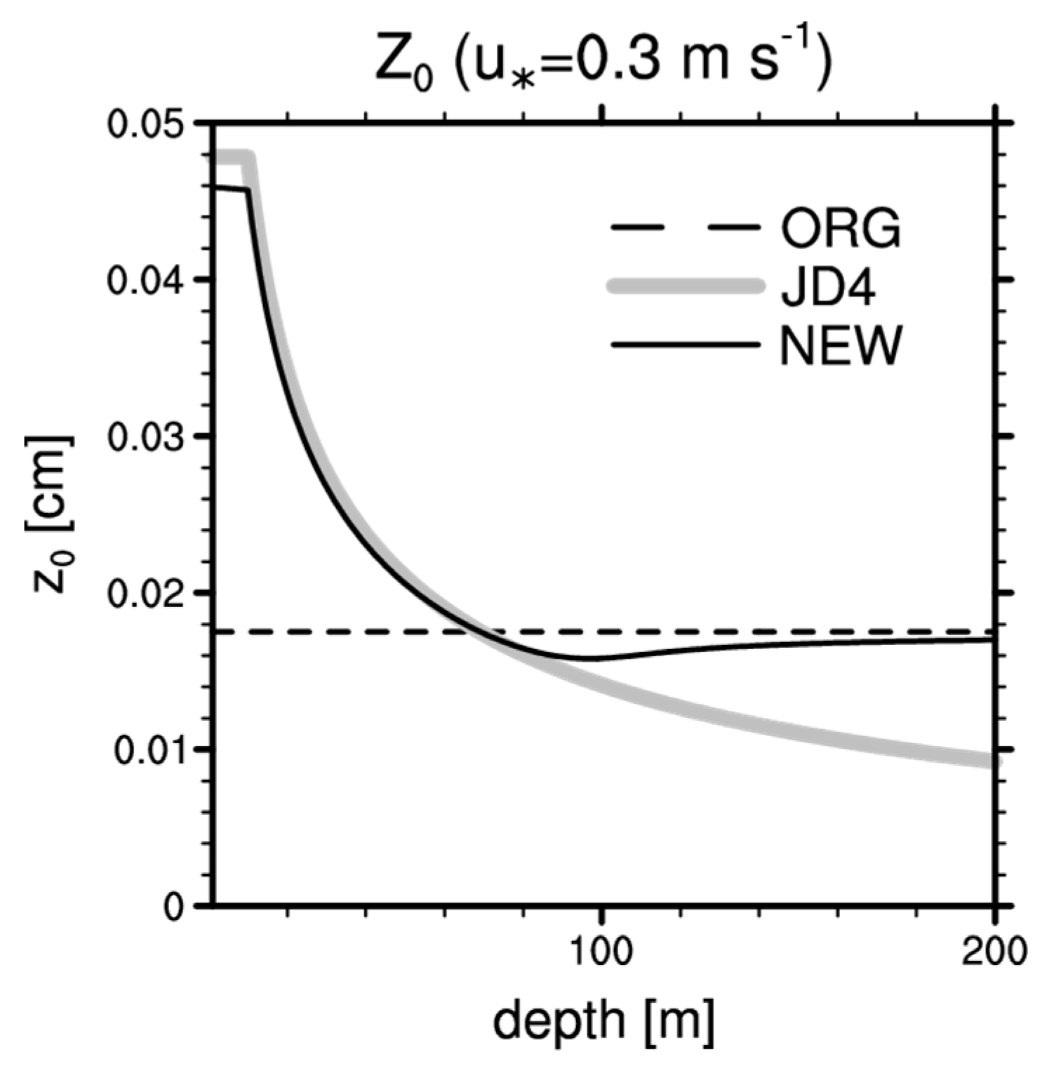
In the Advanced Research Weather Research and Forecasting model (WRF-ARW) [10] used in this study, sea-surface roughness length ( z 0 ) is represented as a function of friction velocity by the revised version of the Charnock (1955) [5] relationship [7] (dashed line in Figure 1) as follows:
z 0 , C h = ( a g ) u + 0.11 υ / u
where a is the Charnock parameter, which is assumed to be 0.0185, g is the gravitational acceleration, u is the friction velocity, and ν is the kinematic viscosity (1.5×10⁻⁵ m2 s−1). The second term on the right side of Equation (1) is to make surface roughness length depend on kinematic viscosity, rather than the Charnock parameter, for light–wind condition. The sea-surface roughness length in other numerical models is also calculated using similar formulas, and the Charnock parameter in atmospheric models is generally assumed to be a constant value representing the average state of the sea.
In order to examine the effects of water depth in the sea-surface roughness calculation, we used the formula suggested by Jiménez and Dudhia (2018) [9] for shallow waters (their Equation (4)) as
z 0 , J D = exp ( 2.7 u 1.8 / b u + 0.17 / b ) ,
b = 1 30 ln ( 1260 max ( d , 10 ) ) ,
where d is water depth (m) (gray line in Figure 1). Equation (2) is adopted for shallow waters with a depth less than 100 m, and the value of d is assumed to be 10 m when the depth is shallower than 10 m. To avoid a discontinuity in sea-surface roughness length values at a depth of 100 m, we combine the values calculated using Equations (1) and (2) as
z 0 = ( 1 α ) z 0 , J D + α z 0 , C h ,
where α is a weighting factor that depends on the water depth and is calculated as
α = 1 π [ atan ( 1 20 ( d 100 ) + π 2 ) ] .
This weighting factor allows the surface roughness length value to follow the formula suggested by Jiménez and Dudhia (2018) [9] over the shallow waters and approach to values derived using the revised version of the Charnock formula as the water depth increases (black solid line in Figure 1).
The formula suggested by Jiménez and Dudhia (2018) [9] mainly considers the effect of water depth in the sea-surface roughness length calculation. They mentioned that other factors, such as fetch and wave age also affect the surface roughness length over shallow waters. Their formula, which is based on limited observations, may require further assessment using observations with extended spatiotemporal ranges to test its reliability. However, the aim of this study is not to improve model performance, but to investigate the impact of considering water depth in surface roughness on atmospheric features.

2.2. Numerical Experiments

The model used for numerical simulation in this study is the WRF-ARW version 4.0 [10]. For physical processes, the WRF-Single-Moment 5-class cloud microphysics scheme (WSM5) [11]; the simplified Arakawa–Shubert (SAS) deep convection scheme [12] modified by Han et al. (2016) [13]; the Rapid Radiative Transfer Model for general circulation models (RRTMG) [14] for shortwave and longwave radiations; the Yonsei University (YSU) boundary layer scheme [15] that is a non-local closure scheme; the Noah land surface scheme [16], and the revised Monin–Obukhov surface layer scheme [17] were used. Three-dimensional simulations were performed in three one-way nested domains in East Asia with a horizontal grid spacing of 27 km (domain 1; D1, with 178 × 150 grid points), 9 km (domain 2; D2, with 259 × 223 grid points), and 3 km (domain 3; D3, with 400 × 382 grid points) (Figure 2). D3 encompasses the Korean Peninsula and the shallow waters (the Yellow Sea) between the Korean Peninsula and the eastern part of China. In the vertical direction, 51 levels were used from the surface to 50 hPa. The National Centers for Environmental Prediction (NCEP) final analysis (FNL) data with a horizontal resolution of 1 degree were used as initial and boundary conditions, and sea-surface temperature (SST) was provided from the NCEP daily real-time global SST analysis [18], with a horizontal resolution of 0.5 degree. To prevent the drift of synoptic-scale features, the spectral nudging method was employed. From the FNL data, large-scale information with wavenumbers less than or equal to 4, 2, and 1 was nudged into D1, D2, and D3, respectively. For water depth information, the General Bathymetric Chart of the Oceans (GBECO) 2014 Grid with a horizontal resolution of 30 arc second, which was released by the British Oceanographic Data Centre (BODC), was used.
Two experiments were performed: (1) a control (CTL) experiment using the original formula (Equation (1)) to calculate the sea-surface roughness length without consideration of water depth, and (2) an experiment using a modified formula (Equation (4)) of sea-surface roughness length considering water depth (Z0MOD experiment). The simulation was initiated from 00 UTC 24 June 2017 and integrated for 38 days, to 00 UTC 1 August 2017. The output in D3 was temporally averaged during July 2017, and that was analyzed in this study.

3. Results and Discussion

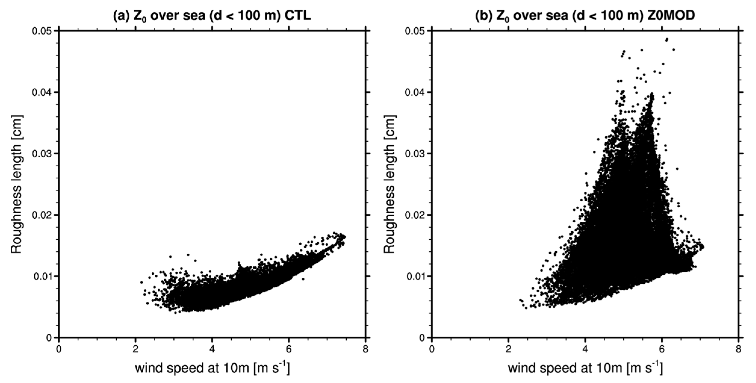
The distribution of surface roughness lengths over shallow waters with a depth less than 100 m is shown in Figure 3. In the CTL experiment, surface roughness lengths generally show an increase, with an increase in wind speed except for wind speeds of less than ~3 m s−1. For wind speed less than ~3 m s−1, the surface roughness lengths increase with a decrease in wind speed—likely because the contribution of the second term on the right side of Equation (1) increases with a decrease in wind speed. In the Z0MOD experiment, the surface roughness lengths are higher than in the CTL experiment, especially for wind speeds between ~4 m s−1 and ~6 m s−1. When the wind speed is less than 3 m s−1, surface roughness is generally lower than that in the CTL experiment because the term considering the light-wind conditions is absent in the revised formula for shallow waters (Equation (2)). Additionally, maximum wind speed recorded in the Z0MOD experiment is lower than that in the CTL experiment. This implies that, in the Z0MOD experiment, the wind speed at 10 m over shallow waters is reduced due to an increase in surface roughness length.
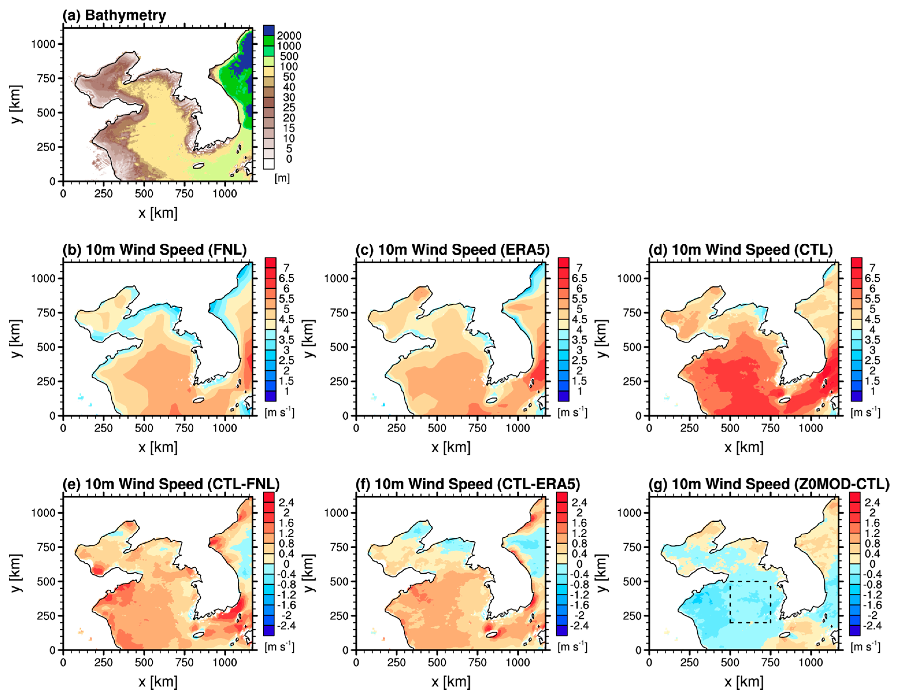
The bathymetry in D3 indicates that the sea is shallower than 100 m across a large area of the domain except for the eastern part (brown and yellow, sub-figure a in Figure 4). This is especially evident for the Yellow Sea, which is located between China and the Korean Peninsula. That is why this area was chosen as experimental domain. Over shallow waters, wind speed at 10 m is generally overestimated in the CTL experiment compared to in the FNL data (Figure 4b,d,e) and the fifth generation of European Center for Medium-range Weather Forecasts (ECMWF) atmospheric re-analyses of global climate (ERA5) data (Figure 4c,d,f). Near-surface wind speed over the coastal region is often overestimated in atmospheric models that are not coupled with ocean and wave models (e.g., [19]). Due to an increase in sea-surface roughness length over shallow waters in the Z0MOD experiment, wind speed at 10 m over the Yellow Sea is found to be lower in the Z0MOD experiment than in the CTL experiment (Figure 4g). This alleviates the wind speed bias, although the reduction is not enough to compensate for the positive bias of wind speed.
Figure 5 shows a comparison with the surface observational dataset including buoy and ship measurements, which is used for the data assimilation system of the Korean Integrated Model [20,21]. Since data are sparse and located at different points depending on the measurement time, 10 July 2017—when the number of measurement points is relatively large—was selected for comparison. The wind speed at 10 m in the CTL experiment is generally overestimated over the Yellow Sea compared to that in the observational dataset (Figure 5a–c), which is consistent with the comparison to the FNL and ERA5 data, and the bias is alleviated in the Z0MOD experiment (Figure 5d). The wind speed in the southeastern part of the domain is underestimated. Underestimation of wind speed in this part is also found in the comparison to the FNL and ERA5 data for the corresponding date (not shown). In this part, the wind speed at 10 m is enhanced overall by considering water depth in the sea-surface roughness length calculation (Figure 5d).
Since near-surface wind could be sensitive to the boundary layer and surface layer schemes used, two additional simulations were conducted during 1–10 July 2017 using (i) Mellor–Yamada–Nakanishi–Niino (MYNN) level 2.5 boundary layer scheme [22], which is a local closure scheme, and (ii) MYNN level 2.5 boundary layer and MYNN surface layer schemes. The overestimation of wind speed at 10 m shown in Figure 4 is also found in both simulations, although the magnitude of overestimation is different between simulations, and the bias is alleviated by considering water depth in the sea-surface roughness length calculation (not shown). The simulation was also performed during January 2017. An overestimation of wind speed at 10 m is found over the Yellow Sea, but its reduction in the Z0MOD experiment is smaller than in July (not shown). This is likely because the wind speed at 10 m over the Yellow Sea is stronger in January than in July and the enhancement of sea-surface roughness length over shallow waters is less significant for higher wind speeds, as expected in Figure 3.
The vertical profile of wind speed over the Yellow Sea (dashed box in Figure 4g) is also calculated (Figure 6). The wind speed at 10 m is higher in the CTL experiment (blue solid line) than in the FNL (black solid line) and ERA5 data (black dashed line), and this overestimation extends to the mid troposphere (~9 km). In contrast, above ~9 km, the wind speed in the CTL experiment is underestimated compared to that in the FNL and ERA5 data. The difference between the CTL experiment and the FNL/ERA5 data reaches ~3 m s−1 in the upper levels. This large difference occurs as a result of a shift in the location of a jet and is because the profile is calculated for a small area. In the Z0MOD experiment (red solid line), wind speed at low levels below ~7 km is reduced compared to that in the CTL experiment, in which the wind speed is overestimated, and a decrease in the wind speed is more significant above ~1.5 km than near the surface. As a result, wind speed in the Z0MOD experiment is relatively close to that in the FNL and ERA5 data near the surface, but lower than that in the FNL and ERA5 data between ~1.5 km and ~5.5 km. The effect of considering water depth in sea-surface roughness length calculation is not localized to near-surface levels, but extends into the upper troposphere. Above ~7 km, wind speed increases by considering depth-dependent sea-surface roughness. In particular, the jet in the upper troposphere is largely enhanced in the Z0MOD experiment. Since wind speed at this level is underestimated in the CTL experiment compared to the FNL and ERA5 data, the modified surface roughness in the Z0MOD experiment acts to alleviate this bias. In the present experiments, bias in the CTL experiment is overcompensated in the Z0MOD experiment, and therefore, the Z0MOD experiment overestimates the wind speed in the upper troposphere.
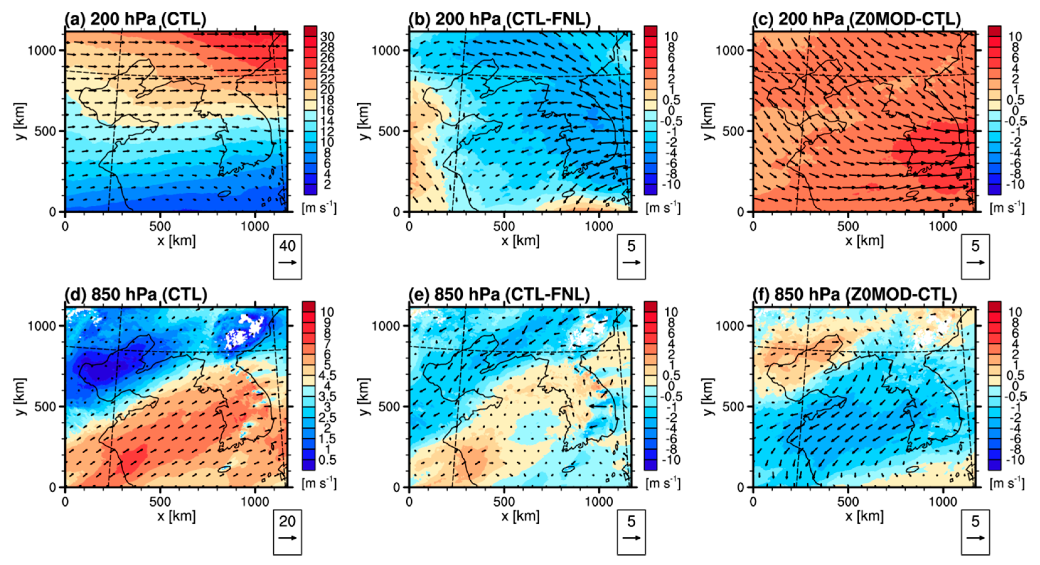
The distributions of upper (200 hPa) and lower (850 hPa) tropospheric horizontal winds are shown in Figure 7. In the CTL experiment, westerlies at 200 hPa, the speed of which increases with latitude (Figure 7a), are underestimated compared to those in the FNL data across most of the domain (Figure 7b). In the Z0MOD experiment, the westerlies are strengthened as shown in Figure 6, and the northwesterly component is enhanced in the northern part of the domain (Figure 7c). The difference in 200 hPa wind between the two experiments (Z0MOD–CTL) has opposite sign to that of bias in the CTL experiment against the FNL data (compare Figure 7b,c). However, the changes occurring due to the modified roughness length overcompensate for the bias and this makes the Z0MOD experiment have the opposite bias to that seen in the CTL experiment. Enhanced westerlies and north-westerlies in the southern and northern part of the domain, respectively, are related to changes in wind in the lower levels. At 850 hPa, the southwesterly flow is dominant (Figure 7d) and this low-level jet is slightly overestimated over the Yellow Sea (Figure 7e). The southwesterly flow is weakened in the Z0MOD experiment (Figure 7f), and this weakens the convergence over the Yellow Sea (not shown). At 200 hPa, changes in flow influenced by modified sea-surface roughness length lead to a decrease in divergence, which could be related to weakened convergence at the lower levels. Over the Yellow Sea, the updraft is also found to be weaker in the Z0MOD experiment than in the CTL experiment (not shown) due to the weakened lower tropospheric convergence and upper tropospheric divergence.
Figure 8 compares the zonal component of wind distribution between the two experiments. As shown in Figure 7, the modified sea-surface roughness length has led to an increase in zonal wind at 200 hPa across the entire domain, especially in the southern part where the wind speed is relatively low (Figure 8c). At 850 hPa, the zonal wind is reduced largely over the Yellow Sea where wind speed is relatively high in the CTL experiment while there are some increases in the northern part of the domain (Figure 8f). Modulated wind in the lower and upper troposphere changes the vertical wind shear. Since zonal wind increases with height (Figure 8a,d), a positive vertical difference is shown in the CTL experiment (Figure 8g). This vertical wind shear is relatively weaker compared to that in the FNL data due to overestimated (underestimated) lower (upper) level wind speeds. Weakened wind speed in the lower troposphere and enhanced wind speed in the upper troposphere result in an increase in vertical wind shear in entire domain (Figure 8i), especially in the southern part of the domain that includes the Yellow Sea. This increase in vertical wind shear of zonal wind contributes to changes in temperature.
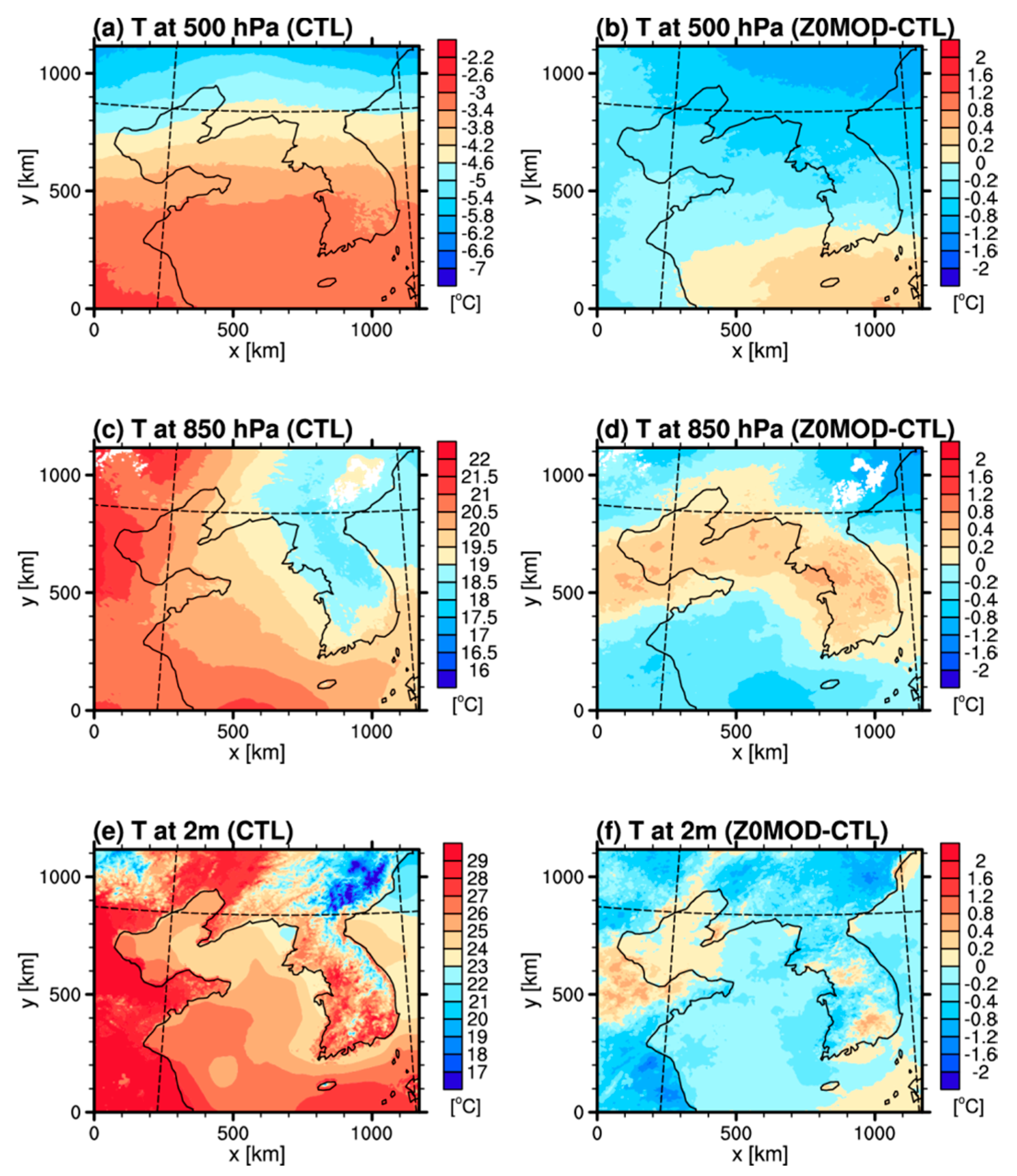
Figure 9 shows the effect on temperature. At 500 hPa, the modified sea-surface roughness length decreases temperature overall, except over the southern part of the domain, and the cooling effect is stronger at higher latitudes (Figure 9b). This enhances the meridional gradient of temperature, which is negative (Figure 9a). The enhanced negative meridional temperature gradient is related to an increase in the vertical wind shear of zonal wind through the thermal wind relationship. A lag-correlation analysis between the changes in the vertical wind shear of zonal wind and the meridional gradient of 500 hPa temperature indicates that changes in the two variables are highly correlated at lags between 0 and 6 h, when the wind shear change leads to a temperature change (not shown). At 850 hPa, the modified sea-surface roughness length leads to a decrease in temperature over the southern part of the domain, along with an increase in the northern part of the Yellow Sea and the Korean Peninsula (Figure 9d). The temperature at 850 hPa is found to be affected by near-surface temperature (e.g., temperature at 2 m), which is also decreased over sea overall (Figure 9f). Additionally, low-level cooling over the Yellow Sea is found to be partly due to colder air advection by the northeasterly flow induced by the modified sea-surface roughness length.

4. Summary and Conclusions

Sea-surface roughness length was modified over shallow waters considering the effect of water depth, and its impact is investigated through a regional climate simulation during a boreal summer. The formula considering water depth suggested by Jiménez and Dudhia (2018) [9] was used only over shallow waters, and the revised version of the formula proposed by Charnock (1995) [5] was used for the open ocean. By using a modified formula of sea-surface roughness length that took water depth into consideration, surface roughness length increased over shallow waters, leading to a direct decrease in near-surface wind speeds. As a result, the overestimation of near-surface wind speeds compared to those in the FNL data was alleviated. Lower tropospheric wind speeds were also reduced over shallow waters.
The effects of increased sea-surface roughness over shallow waters were not localized to low-level wind, but extended to the upper tropospheric wind. In the upper troposphere, wind speed was largely increased. The upper tropospheric wind speed was underestimated in the control experiment. Therefore, the enhancement of wind speed by the modified sea-surface roughness length acted to reduce the underestimation of wind speed. In the present simulations, however, the bias was overcompensated and the wind speed in the upper troposphere was overestimated in the experiment with modified sea-surface roughness length. Decreased wind speed in the lower troposphere and increased wind speed in the upper troposphere led to the enhancement of vertical wind shear between the upper and lower troposphere. The vertical difference in zonal wind between 200 hPa and 850 hPa increased, and as a result, the meridional temperature gradient at 500 hPa increased through the thermal–wind relationship. The low tropospheric temperature was also found to be affected by a modulated wind structure.
This study shows that a change in sea-surface roughness length modulates upper-tropospheric wind and temperature, as well as low-level atmospheric features. This modulation is not localized over shallow waters, but is apparent in the entire experimental domain. Additionally, positive changes are shown that help compensate for the bias in the model, although they are excessive in the upper troposphere. This implies that a proper representation of surface properties over the ocean is important in the simulation of upper level atmospheric features as well as of low-level circulation. This study mainly considers the effect of water depth in sea-surface roughness length. There are a number of other factors that could affect sea-surface roughness, including those that represent the state of the ocean, such as wave age, wavelength, and the phase speed of waves. The effects of these factors can be analyzed further by coupling ocean and wave models to atmospheric models.
Author Contributions

Conceptualization, Y.C.K., Y.H.L., S.-Y.K., S.-Y.H. and D.-E.K.; methodology, S.-Y.K. and S.-Y.H.; software, S.-Y.K.; validation, S.-Y.K.; investigation, S.-Y.K.; data curation, S.-Y.K. and D.-E.K.; writing—original draft preparation, S.-Y.K.; writing—review and editing, S.-Y.K., and S.-Y.H.; visualization, S.-Y.K. All authors have read and agreed to the published version of the manuscript.

Funding

This research was funded by the Korea Meteorological Administration (KMA).

Acknowledgments

This work has been carried out through the R&D project on the development of global numerical weather prediction systems of the Korea Institute of Atmospheric Prediction Systems (KIAPS) funded by the Korea Meteorological Administration (KMA). The NCEP FNL data are available from the Computational and Information Systems Laboratory (CISL) Research Data Archive (RDA; http://rda.ucar.edu/datasets/ds083.2), and ERA5 data are available from the Copernicus Climate Change Service Climate Data Store (CDS) (https://cds.climate.copernicus.eu/). The GBECO 2014 Grid data are available from the BODC (http://bodc.ac.uk).

Conflicts of Interest

The authors declare no conflict of interest.

References

  1. Hsu, S.A. A dynamics roughness equation and its application to wind stress determination at the air-sea interface. J. Phys. Oceanogr. 1974, 4, 116–120. [Google Scholar] [CrossRef] [Green Version]
  2. Smith, S.D.; Anderson, R.J.; Oost, W.A.; Kraan, C.; Maat, N.; de Cosmo, J.; Katsaros, K.B.; Davidson, K.L.; Bumke, K.; Hasse, L.; et al. Sea surface wind stress and drag coefficients: The HEXOS results. Bound. Layer Meteorol. 1992, 60, 109–142. [Google Scholar] [CrossRef] [Green Version]
  3. Johnson, H.K.; Højstrup, J.; Vested, H.J.; Larsen, S.E. On the dependence of sea surface roughness on wind waves. J. Phys. Oceanogr. 1998, 28, 1702–1716. [Google Scholar] [CrossRef]
  4. Taylor, P.K.; Yelland, M.J. The dependence of sea surface roughness on height and steepness of the waves. J. Phys. Oceanogr. 2001, 31, 572–590. [Google Scholar] [CrossRef] [Green Version]
  5. Charnock, H. Wind stress on a water surface. Q. J. R. Meteorol. Soc. 1955, 81, 639–640. [Google Scholar] [CrossRef]
  6. Donelan, M.A. Air-sea interaction. In Ocean Engineering Science; LeMehaute, B., Hanes, D.M., Eds.; John Wiley: New York, NY, USA, 1990; Volume 9, pp. 239–292. [Google Scholar]
  7. Hersbach, H. Sea-Surface Roughness and Drag Coefficient as Function of Neutral Wind Speed; ECMWF Technical Memorandum 630; ECMWF: Reading, UK, 2010; p. 6. [Google Scholar]
  8. Arya, S.P. Introduction to Micrometeorology, 1st ed.; Academic Press: San Diego, CA, USA, 1988; p. 303. [Google Scholar]
  9. Jiménez, P.A.; Dudhia, J. On the need to modify the sea surface roughness formulation over shallow waters. J. Appl. Meteorol. Climatol. 2018, 57, 1101–1110. [Google Scholar] [CrossRef]
  10. Skamarock, W.C.; Klemp, J.B.; Dudhia, J.; Gill, D.O.; Liu, Z.; Berner, J.; Wang, W.; Powers, J.G.; Duda, M.G.; Barker, D.M.; et al. A Description of the Advanced Research WRF Model Version 4; NCAR Technical Note NCAR/TN-556+STR; Mesoscale and Microscale Meteorology (MMM) Division, NCAR: Boulder, CO, USA, 2019. [Google Scholar]
  11. Hong, S.-Y.; Dudhia, J.; Chen, S.-H. A revised approach to ice microphysical processes for the bulk parameterization of clouds and precipitation. Mon. Weather Rev. 2004, 132, 103–120. [Google Scholar] [CrossRef]
  12. Hong, S.-Y.; Pan, H.-L. Convective trigger function for a mass flux cumulus parameterization scheme. Mon. Weather Rev. 1998, 126, 2599–2620. [Google Scholar] [CrossRef]
  13. Han, J.-Y.; Hong, S.-Y.; Lim, K.-S.S.; Han, J. Sensitivity of a cumulus parameterization scheme to precipitation production representation and its impact on a heavy rain event over Korea. Mon. Weather Rev. 2016, 144, 2125–2135. [Google Scholar] [CrossRef]
  14. Iacono, M.J.; Delamere, J.S.; Mlawer, E.J.; Shephard, M.W.; Clough, S.A.; Collins, W.D. Radiative forcing by long-lived greenhouse gases: Calculation with the AER radiative transfer models. J. Geophys. Res. 2008, 113, D13103. [Google Scholar] [CrossRef]
  15. Hong, S.-Y.; Noh, Y.; Dudhia, J. A new vertical diffusion package with an explicit treatment of entrainment processes. Mon. Weather Rev. 2006, 134, 2318–2341. [Google Scholar] [CrossRef] [Green Version]
  16. Chen, F.; Dudhia, J. Coupling an advanced land surface-hydrology model with the Penn State-NCAR MM5 modeling system. Part I: Model implementation and sensitivity. Mon. Weather Rev. 2001, 129, 569–585. [Google Scholar] [CrossRef] [Green Version]
  17. Jiménez, P.A.; Dudhia, J.; González-Rouco, J.F.; Navarro, J.; Montávez, J.P.; García-Bustamante, E. A revised scheme for the WRF surface layer formulation. Mon. Weather Rev. 2012, 140, 898–918. [Google Scholar] [CrossRef] [Green Version]
  18. Thiébaux, J.; Rogers, E.; Wang, W.; Katz, B. A new high-resolution blended real-time global sea surface temperature analysis. Bull. Am. Meteorol. Soc. 2003, 84, 645–656. [Google Scholar] [CrossRef] [Green Version]
  19. Li, H.; Kanamitsu, M.; Hong, S.-Y.; Yoshimura, K.; Cayan, D.R.; Misra, V. A high-resolution ocean–atmosphere coupled downscaling of the present climate over California. Clim. Dyn. 2014, 42, 701–714. [Google Scholar] [CrossRef]
  20. Hong, S.-Y.; Kwon, Y.C.; Kim, T.-H.; Kim, J.-E.E.; Choi, S.-J.; Kwon, I.-H.; Kim, J.; Lee, E.-H.; Park, R.-S.; Kim, D.-I. The Korean Integrated Model (KIM) system for global weather forecasting. Asia Pac. J. Atmos. Sci. 2008, 54, 267–292. [Google Scholar] [CrossRef]
  21. Kang, J.-H.; Chun, H.-W.; Lee, S.; Ha, J.-H.; Song, H.-J.; Kwon, I.-H.; Han, H.-J.; Jeong, H.-B.; Kwon, H.-N.; Kim, T.-H. Development of an observational Processing Package for Data Assimilation in KIAPS. Asia Pac. J. Atmos. Sci. 2008, 54, 303–318. [Google Scholar] [CrossRef]
  22. Nakanishi, M.; Ninno, H. An improved Mellor-Yamada level-3 model: Its numerical stability and application to a regional prediction of advection fog. Bound. Layer Meteorol. 2006, 119, 397–407. [Google Scholar] [CrossRef]
Figure 1. Sea-surface roughness length (cm) with respect to water depth (m) calculated using original formula (Equation (1), dashed); formula suggested by Jiménez and Dudhia (2018) [9] (Equation (2), gray), and a combination of both formulas using a weighting factor that depends on water depth (black solid). Friction velocity is assumed to be 0.3 m s−1.
Atmosphere 10 00818 g001
Figure 2. Model domains and ocean bathymetry (m, shaded).
Atmosphere 10 00818 g002
Figure 3. Sea-surface roughness length (cm) over shallow waters with a depth less than 100 m as a function of wind speed at 10 m in the (a) control (CTL) and (b) sea-surface roughness length considering water depth (Z0MOD) experiments.
Atmosphere 10 00818 g003
Figure 4. (a) Bathymetry (m) and wind speed at 10 m (m s-1) in the (b) final analysis (FNL) data, (c) ECMWF reanalysis (ERA5) data, (d) CTL experiment, (e) difference between the CTL experiment and the FNL data (CTL-FNL), (f) difference between the CTL experiment and the ERA5 data (CTL-ERA5), and (g) difference between the Z0MOD and CTL experiments (Z0MOD-CTL). The dashed box in (g) indicates the area where the wind speed is averaged for profile in Figure 6.
Atmosphere 10 00818 g004
Figure 5. Wind speed at 10 m (m s−1) on 10 July 2017 at observational points in the (a) CTL experiment, and the (b) surface observational (OBS) data; (c) difference between the CTL experiment and the OBS data (CTL-OBS); (d) difference between the Z0MOD and CTL experiments (Z0MOD-CTL).
Atmosphere 10 00818 g005
Figure 6. Wind speed profile averaged over the area indicated by dashed box in Figure 4g in the CTL (blue solid line) and Z0MOD (red solid line) experiments and FNL (black solid line) and ERA5 (black dashed line) data.
Atmosphere 10 00818 g006
Figure 7. Horizontal wind vector and speed (shaded) at (ac) 200 hPa and (df) 850 hPa in (a,d) the CTL experiment, (b,e) difference between the CTL experiment and FNL data (CTL–FNL), and (c,f) difference between the Z0MOD and CTL experiments (Z0MOD–CTL).
Atmosphere 10 00818 g007
Figure 8. Zonal wind at (ac) 200 hPa, (df) 850 hPa, and (gi) vertical difference between 200 hPa and 850 hPa (200 hPa–850 hPa) in the (a,d,g) CTL and (b,e,h) Z0MOD experiments, and (c,f,i) difference between the Z0MOD and CTL experiments (Z0MOD–CTL).
Atmosphere 10 00818 g008
Figure 9. Temperature at (a,b) 500 hPa, (c,d) 850 hPa, and (e,h) 2m in (left) the CTL experiment and (right) difference between the Z0MOD and CTL experiments (Z0MOD–CTL).4. Summary and Conclusions.
Atmosphere 10 00818 g009