1. Introduction
Data assimilation is a process by which observations are integrated into a model of the atmosphere thereby changing the model state and its associated forecast. Tropospheric observations related to dynamical variables such as temperature, wind, and humidity are continuously collected and routinely assimilated in weather prediction models. In the stratosphere, there are fewer meteorological observations available and these are mostly related to temperature, but there are, however, several research satellites measuring chemical composition in this region [
1]. Important missions began in the early 1990s with the Upper Atmosphere Research Satellite (UARS) [
2,
3,
4] followed by the Environmental Satellite Envisat [
5,
6,
7] and NASA’s Earth Observing System (EOS) Aura [
8,
9]. Instruments on board these satellites typically perform measurements which are tangent to the atmosphere (also called limb soundings) and provide height-resolved retrievals of a number of chemical species as well as temperature. Chemical transformations, especially those related to stratospheric ozone, have an impact on the temperature, while winds change the distribution of chemical tracers (i.e., long-lived species). A natural question which then arises is “
To what extent does the assimilation of chemical observations, and in particular those provided by limb measurements, impact the meteorology on time scales relevant to numerical weather prediction?” This is the main objective of this study. In Part I we focused on modelling aspects and introduced the coupled model GEM-BACH (GEM with the Belgian Atmospheric Chemistry model). Here we will discuss how these research satellite observations can provide useful information, and in particular, using weak and strong data assimilation coupling.
Coupled data assimilation is a relatively new area of research and development, where assimilation systems can broadly be classified as either weakly or strongly coupled [
10,
11,
12]. In weakly coupled data assimilation system, each geophysical component (e.g., chemistry, meterology) has its own independent analysis. The analyses are then used to initialize a coupled model, which produces a coupled model forecast (i.e., the coupling arises through the model forecast and not through the analysis). In a strongly coupled data assimilation system, the analysis is carried out on all variables together. Thus, observations of one geophysical component can have a direct impact on the analysis of the other geophysical component. Weak and strong data assimilation coupling strategies were developed for atmosphere-ocean [
12,
13,
14,
15,
16,
17,
18,
19,
20,
21,
22,
23,
24,
25] and atmosphere-land-surface coupled systems [
26,
27,
28,
29,
30].
Coupled meteorology–chemistry data assimilation has primarily been examined in the context tropospheric aerosol-radiation interaction, on short time-scales [
31,
32,
33], on subseasonal time scales [
34] and decadal time scales [
35] (also see [
36] for a review of chemical data assimilation). It was also used to estimate parameters in the activation of aerosols into cloud droplets [
37], and in determining cross-covariance between temperature and constituents (O
3, NO
2, and SO
2) using the coupled tropospheric model WRF-CHEM with an ensemble based approach [
38]. Coupling can also occur through coupled observation operators. For example, infrared channels of operational meteorological satellites are sensitive to ozone and CO
2 and can benefit from using an ozone assimilation [
39] and a CO
2 assimilation [
40].
Data assimilation coupling in the stratosphere was also investigated in perspective of weak coupling through ozone–radiation interaction, and as strong coupling using the tracer-wind relation. Weak coupling was investigated at numerical weather prediction centers, such as ECMWF, by considering the ozone–radiation interaction [
41] and at the Canadian Meteorological Center (CMC) with the experimental model GEM-BACH [
42]. The experiments conducted at ECMWF (European Center for Medium Range Forecasting) were performed with a linearized ozone chemistry and using nadir-sounding stratospheric measurements, whereas those at CMC used a relatively low resolution model but with the full stratospheric chemistry and using limb sounding observations. The CMC study showed an impact on the meteorological forecast skill in the lower stratosphere.
Strong data assimilation coupling has been considered in the context of using chemical tracer observations to infer winds. Some earlier studies using an extended Kalman filter with a simplified two-dimensional transport model showed that wind recovery is very sensitive to the accuracy of chemical observations, and to the concentration fields having sufficient horizontal gradients and with small data voids [
43]. It was also shown that constituents in zones of convergence could only determine the winds nearby. Experiments conducted with a one-dimensional model also showed that wind information can still be obtained in the case of a flat concentration field if there are gradients in the concentration error covariances [
44]. Using the barotropic vorticity equation with a 4D-Var assimilation system, Riishøjgaard [
45] examined the issues of data density and length of the assimilation window, and arrived at similar conclusions. Using column measurements of ozone with a NWP (Numerical Weather Prediction) model and 4D-Var method, a small improvement in the winds was obtained using simulated observations, but a deterioration using real observations [
46]. The negative impact was suspected to result from observational bias. In another study using an operational NWP model with a 4D-Var assimilation system, a small impact (about 0.1 m s
−1) was found on zonal wind with no reduction of error standard deviation [
47]. These rather unsuccessful results conducted in an operational context suggested that additional studies were necessary. Using an ensemble Kalman filter and an intermediate-complexity model, Milewski and Bourqui [
48] demonstrated that information about the ozone-wind cross-covariance is essential in constraining dynamical fields when ozone only is assimilated. Moreover they showed that a further reduction in error can be obtained with an ensemble Kalman smoother [
49]. In a series of studies using 4D-Var and the ensemble Kalman filter, Allen et al. [
50,
51,
52] showed that poorly-specified observation error could lead to an increase in RMS wind error, that observational coverage is important such that wind extraction could be improved if several chemical tracers were used, and that the balance between wind and temperature could be offset by the wind recovery from tracer measurements. We should note that the wind extraction from tracer observation is part of a more general class of joint state-parameter estimation problems (e.g., [
53,
54]).
The present study took place in the period 2005–2009 with funding, in part, from ESA/ESTEC [
55]. This article, henceforth referred to as Part II, summarizes the data assimilation aspects. First, in
Section 2, we present the extension of the CMC variational assimilation system to include chemical variables where we discuss in particular the analysis splitting and preconditioning, the extension of balance operators with chemical variables, and the validity of an incremental formulation of adjoint tracer operators for 4D-Var assimilation of long-lived species. In
Section 3 we describe the error statistics of chemical variables using the Hollingsworth–Lönnberg method to estimate the error variances, and using the Canadian Quick Covariance (CQC) method to obtain non-separable error correlations. We also discuss the method and issues related to the cross-covariances between temperature and ozone. In
Section 4 and
Section 5 we illustrate the benefits of using limb sounding temperatures from the MIPAS instrument on board Envisat to improve the AMSU-A bias correction and better simulation of temperature and transport in the stratosphere. We then discuss a weak coupling data assimilation experiment involving ozone and its impact on meteorological forecasts and show that a simplified linearized ozone chemistry gives comparable results to the full chemistry in terms of impact on thermodynamics. Then in
Section 7 and
Section 8 we discuss results from strong coupling experiments, first in a 3D-Var context using a balance operator between ozone and temperature, and then in 4D-Var assimilation of several long-lived species, i.e., O
3, CH
4, and N
2O to correct the winds.
2. Extension of 3D-Var and 4D-Var for Chemical—Meteorological Coupling
The assimilation system scheme used here consists of a model integration step to obtain a six-hour forecast (called the background state), and an assimilation step in which observations are used to correct the background state and obtain an analysis. This analysis is then used to initialize the next six-hour forecast, and the cycle is repeated. In this study, the assimilation step employs a variational analysis solver that can be run in one of three modes:
3D-Var: In this case, all observations collected over the six-hour assimilation window are assumed to be valid at the central time. Observation departures from the model state (called innovations) are computed with respect to the background state valid at the central time of the window [
56].
3D-FGAT (First Guess at Analysis Time): This scheme is a variant of 3D-Var in which the innovations are evaluated by comparing each observation with the model output valid at the observation time [
57] (actually closest to a 1-hour bin). This is the default configuration used in all 3D-Var experiments in this study.
4D-Var: Extending 3D-Var to 4D-Var can be achieved by including the forward model integration as part of the observation operator (the observation operator computes the model equivalent of the observation) [
58,
59].
It is generally assumed in variational analysis that observation errors and background errors are uncorrelated, both unbiased, and Gaussian distributed. Producing a minimum variance estimate (or maximum a posteriori estimate for nonlinear observation operator), called the analysis, leading numerically to a large-scale minimization problem of a quadratic function that can be solved by unconstrained minimization techniques. This requires suitable preconditioning, and an adjoint observation operator (that is equivalent of a matrix transpose of the Jacobian of the non-linear observation operator).
4D-Var mode also requires the adjoint of the linearized (prognostic) model, commonly called the adjoint model. The linearization is made about a nonlinear model solution, but in the incremental form of 4D-Var, the linearized model is not required to be at the same resolution nor contain the same physics. In this study, however, the linearized model on which the adjoint model is based is at the same resolution (following the discussion in Section 6 Part I) but has no adjoint of ozone–radiation interaction and no adjoint of chemistry. All 4D-Var chemical data assimilation experiments were conducted using only long-lived species treated as passive tracer (over a period of six hours; the time length of the 4D-Var time window).
Background error covariances and observation error covariances are needed to compute a minimum variance estimate. The background error correlation model used in this study is, for each variable, homogeneous and isotropic (i.e., invariant under rotation) on a sphere, and non-separable, meaning that the vertical and horizontal correlation structures are interconnected. The cross-variable error correlations are obtained by a transformation of variables, involving what are called balance operators obtained from a regression analysis following a Gram–Schmidt orthogonalization procedure (
Section 2.3). For the dynamical model variables, there are balance operators to represent the geostrophic and hydrostatic balance, and also the Ekman balance in the planetary boundary layer. In this study we introduced a balance operator between ozone and temperature that was obtained from either a fully coupled meteorological-chemical model or from a LINearized OZone photochemical model such as LINOZ [
60] (see [
61] for the implementation of LINOZ with semi-Lagrangian transport).
Applying balance operators between variables (when needed) and representing the error correlations in spherical harmonics, it is possible to completely diagonalize the error correlation matrix [
62]. The covariances in physical space and between all variables can then be obtained through a series of transformations on a vector. With this formulation the background error covariance matrix can, in principle, be easily expanded to include other non-meteorological variables. This approach was taken to extend our meteorological data assimilation system to a coupled chemistry-dynamics data assimilation solver. The numerical coding effort began in another Canadian study [
63] and was completed here with cross dynamics-chemistry balance operators and the 4D-Var chemical extension (passive tracer).
The last step of the development concerns the preconditioning, which will be discussed in
Section 2.1. In principle, the control vector should contain all the meteorological and chemical variables and which, in our case, consists of 57 (constituent) + 4 (dynamical) = 61 three-dimensional fields. In developing the preconditioning, it was realized, however, that only the observed variables had to be added to the control variable. In our case, this amounts to 4 + 6 = 10 three-dimensional fields (horizontal winds, temperature, water vapor, O
3, CH
4, NO
2, N
2O, HNO
3, and ClONO
2). As far as unobserved constituents that have correlated errors with observed constituents, their minimum variance estimate can be obtained off-line after the minimization.
2.1. Analysis Splitting between Observed and Unobserved Variables
The state of a chemical-meteorological model comprises of all prognostic meteorological and chemical model variables, which, in our case, represents 61 three-dimensional fields (57 advected chemical species + 4 dynamical variables). In principle, a state estimate should be conducted on all these variables. Yet, only a small fraction of these variables are observed. For example, MIPAS/ESA {5-7] chemical observations are mostly limited to O3, N2O, NO2, CH4, and HNO3. We will derive in this section a computational simplification that allows splitting the analysis into observed and unobserved variables parts.
Let
Z be the complete chemical-meteorological state vector be decomposed into
observed variables
X and
unobserved variables
U, i.e.,
The analysis of all state variables using a 3D-Var algorithm consists of minimizing the following cost function:
where
y denotes the observation vector (i.e., all observations of all observed variables at a given time),
H is the observation operator,
R the observation error covariance matrix, and
B is the full state background error covariance matrix that can be decomposed into:
which includes covariances and cross-covariances between observed and unobserved variables.
Developing a preconditioning for the cost function in Equation (2) with the full state vector
Z we found that the minimization of
can be split into two parts: A minimization of the cost function involving only the observed variables and observations, which takes the form:
and a regression between the analysis increments of the unobserved variables with the increments of the observed variables, of the form:
This property is called
analysis splitting. Note that the cost function in Equation (4) is composed of two parts, the background cost function
and the observation cost function
. We should also note that analysis splitting is quite general, and holds, in particular, when the observation operator is nonlinear (the derivation in presented in
Appendix A), but does not apply to 4D-Var as the
term is not separable in that case.
The concept of analysis splitting is interesting in terms of assimilation coupling and for practical reasons. Consider the behavior of unobserved variables U in either strongly-coupled or weakly-coupled data assimilation system. The analysis increment in a strongly-coupled data assimilation system would use (Equation (5)) as part of the initial condition for a coupled model. In a weakly-coupled data assimilation system, we would use (instead of ) to initialize the unobserved space, and furthermore would be obtained from an uncoupled analysis. That means that, for example, in weakly-coupled chemistry–meteorology data assimilation, , where are meteorological and chemical variables so that in the coupled model the initial condition is given by .
Analysis splitting is also practical as it reduces the optimization state space dimension for the 3D-Var. It also offers the possibility to examine the impact of the analysis on unobserved variables independently of the core variational optimization. In the absence of adequate information about cross-covariances between observed and unobserved variables, the increments of unobserved variables can be selectively removed from of the analysis in a simple manner.
2.2. General Description of the 3D-Var-CHEM
The CMC 3D-Var scheme developed for meteorology [
56] and extended to include chemical variables [
63] was further extended in this study to include cross-covariances between observed variables and between observed and unobserved variables using a balance operator. The general framework of balance operators will be discussed in
Section 2.3 and the associated error statistics in
Section 3.3. Cross-covariances involving chemical variables were estimated point-wise, while the meteorological variable error covariances (and cross-covariances) were computed in spectral space as in by Derber and Bouttier [
64].
The coupled chemical-meteorological model state used in the 3DVar-Chem in Equation (4) consists of
X = (
ψ,
χ,
T, ln(
q),
c1, …,
cN,
ps)
T, where
is the streamfunction,
the velocity potential (not the confuse with
used in the previous sub-section),
T the temperature,
q the (tropospheric) water vapor mixing ratio,
ps the surface pressure and
N observed chemical constituent with mixing ratios
c1, …,
cN. The state vector in 3D Var-Chem is such that all 3D fields are grouped together, followed by the 2D field
ps. As explained in
Section 2.1, the state augmentation is limited only to observed variables/species.
A flow chart of the 3D-Var-Chem (omitting some intermediate steps) is given in
Figure S1 (Supplementary Material). The 3D-Var-CHEM code can be used for: (1) general assimilation, (2) identification of observation outliers (background check), (3) monitoring (determination of O-P only), (4) testing by way of single observation experiments, and (5) stand-alone analysis splitting, i.e., Equation (5).
The minimization of the cost function in Equation (4) is performed after a transformation of variables,
where
, which simplifies the background penalty term to a simple quadratic of the form,
- a transformation step called preconditioning. The minimization is then performed on the transformed variable
using an efficient quasi-Newton algorithm adapted for large-scale problems [
65]. The preconditioning used in 3DVar-Chem follows what is done for the meteorological variables [
56]. The key aspect of this computation resides in the fact that
L times a vector
X, can be obtained as a sequence of operators, without the need to store any large matrices. This property arises principally from the assumption that the horizontal error correlation is assumed to be homogeneous and isotropic on the sphere. For such correlations, the spectral representation is diagonal in spectral space (see for example [
56,
62,
66,
67]). The sequence of operations then becomes as follows: (1) We multiply the spectral representation of the state
with the square root of the spectral coefficient of the correlation model
(which is a diagonal matrix for separable models and bloack diagonal for non-separable correlation model); (2) perform a transform from spectral to physical space. First using a spectral transform
which gives a field on the Gaussian grid, and then followed by an interpolation
from the Gaussian grid to a regular latitude–longitude grid; (3) multiply the resulting fields by the error variances (that takes the form of a diagonal matrix of error standard deviation
); and (4) using balance operators
M (to be define below), transform the primary fields into fields of physical significance accounting for cross-correlations between them. This is how we obtain, for example, the velocity potential from the stream function and an unbalanced velocity potential. This last operation is obtained through a balance operator. In the end, the square root of
is given as
, a sequence of operators.
Before we discuss the balance operators, we should note two things: (1) The CMC 3D-Var system uses a non-separable error correlation model. This means that for each horizontal wavenumber there is a unique vertical correlation matrix, and this introduces a dependence between horizontal and vertical scales; and (2) although it is usual in meteorological applications to perform the minimization on an analysis grid of lower resolution than the model grid (e.g., [
56] and in 4D-Var incremental formulation [
68]), as we argued in Part I, Section 6, the meteorological model and analysis increment, as well as the chemical forecast model and the chemical analysis increment should all be on the same grid, in order to avoid a loss of information.
2.3. Balance Operators
Balance operators have been introduced in meteorological data assimilation to account implicitly for the balance between mass and momentum in the background error covariance either through deterministic relationships (e.g., linear balance equation) [
56,
69,
70,
71] or through statistical regression [
64,
72]. The multilinear regression approach [
72] is particularly useful to define balance operators involving chemical species. In particular the streamfunction
, velocity potential
, temperature
, and ozone
which are known to be correlated, can be transformed into a set of
uncorrelated background error variables (denoted with a superscript
u), as follows:
The transformation from any set of correlated errors to uncorrelated error variables, as in Equation (6), can also be explained geometrically by adopting a Hilbert space representation of the random variables [
73,
74] and followed by Gram–Schmidt orthogonalization procedure (see
Appendix B for a geometrical derivation).
Back-substituting, we recover the transformation from uncorrelated variables to correlated variables, in the form:
where:
In the above we have set to zero (i.e., neglected) all cross-covariances involving the uncorrelated velocity potential, . Equation (8) consists of the balance operators involving the main variables only. The list of variables and their associated balance operator in Equation (7) is actually incomplete. To be complete it should include surface pressure, which follows the same structure as temperature, and humidity, which is assumed to be uncorrelated with any other meteorological variable. In chemistry, we could have also introduced a cross-covariance between long-lived species such as (N2O, CH4) or chemically-related species such as (O3, NO2), but we have not done so here.
From Equation (7) we obtain the background error covariances, which can be rewritten by splitting the covariances into variances and correlations as follows:
where
is a diagonal matrix of error standard deviations for all uncorrelated variables. Note that each correlation matrix
C, is actually represented spectrally as
where
S and
are the spectral direct and inverse transform and
is a diagonal or block-diagonal (
) matrices of spectral coefficients. For computational efficiency, the balance operators in
M are simplified as block diagonal matrices (
) for each latitude with an error variance that depends on height and latitude (using a Legendre polynomial expansion).
To start a 3D-Var or 4D-Var analysis using preconditioning requires the inverse of the square root of
, and, thus, we need to know the inverse of
M, which turns out to be easy to obtain as:
we should also note that computation using the balance operator never involve the computation of an inverse of a large matrix. For example, to compute
we begin by first solving for
in the equation
, then followed by computing
.
2.4. D-Var Tracer Extension
The 3D-Var algorithm can be extended to 4D-Var by including the model integration as part of the observation operator [
58,
59]. The minimization of the 4D-Var cost function with the adjoint of the original model including the full physics can be difficult and computationally demanding. Instead, an incremental formulation of 4D-Var [
68] can be used where the minimization of the 4D-Var cost function is approximated by a series of minimizations involving the adjoint of a tangent linear model with simplified physics and at a lower resolution [
68,
75,
76], called the inner-loop and where its solution is used to update the full model trajectory in an outer-loop. The outer-loop trajectories define new innovations and a new cost function and the method cycles through several outer loops, each of which requires the minimization in an inner loop. At CMC, the physics component of the adjoint model includes only the vertical diffusion, surface drag, orography blocking, stratiform condensation and convection. The simplified adjoint model is also run at a resolution of 1.5° × 1.5°, which is the same resolution as that of the GEM-BACH model. For the chemistry component of GEM-BACH, the adjoint is simplified by considering only the adjoint of advection transport. There is no adjoint of chemistry. The tangent-linear model of semi-Lagrangian advection was discussed in Polavarapu [
77] and the properties of the adjoint in Tanguay and Polavarapu [
78]. The key element in the implementation of 4D-Var for GEM-BACH is that the minimization is performed within the inner loop which uses the tracers of observed species only (with the simplified physics). The outer-loop uses the full chemistry and physics.
4D-Var assimilation of ozone was conducted between 300 hPa and 10 hPa where ozone is long-lived and, thus, be approximated as a passive tracer. To illustrate the validity of the incremental tracer approach for ozone,
Figure 1 shows the observation cost function Jo as a function of iteration. The solid black is the result of the first inner loop (up to iterate 42), while the dashed line refers to the cost function after the first update of the outer loop, during the second inner loop. We observe that the observation cost function is continuous, except for a small adjustment between the last iterate of the first inner loop and the beginning of the second inner loop, thus, indicating no significant issues with the incremental tracer approach.
3. Error Statistics
An accurate estimation of the observation and background error statistics is important in data assimilation as these control (at analysis time) the weight of the observations and the structure functions that spread information in space and to other model variables. The innovations contain the basic information to estimate the observation and background error statistics but this information is actually combined, i.e., not separated in its respective components. Under the assumption that observation errors are spatially uncorrelated and background errors are spatially correlated it is, however, possible to separate the observation and background error statistics. The Hollingsworth–Lönnberg (HL) method [
79,
80] does precisely this and is based on computing the distance between pair of observations usually at fixed locations. Here, we demonstrate that this method can also be used with a polar orbiting limb sounder, such as the MIPAS instrument on board Envisat using the distance between observations profiles along the orbit. With this approach, we were able to derive the observation and background error statistics of the observed chemical species. We should add that there are other methods in observation space that can provide observation and background error statistics, such as Desroziers [
81] and Desroziers and Ivanov [
82] methods, but these are based on different assumptions (see [
83]).
Any of these methods are limited as they can only estimate error statistics of the observed variables in the observation space, which is insufficient to prescribe the error statistics needed for an assimilation system. Additional information can be obtained by using model output methods, such as the ensemble methods and the lagged-forecast method also known as the NMC (National Meteorological Center) method. Ensemble methods require an ensemble of model forecasts, but conducting an ensemble of the GEM-BACH model runs would be computationally demanding, and would require tuning of model error (i.e., inflation) and localization. The lagged-forecast method, widely used in meteorology, uses differences of forecast valid at the same time(s) and is based on having a complete observational coverage. However, Bouttier [
84] argued that the lagged-forecast method is strongly related to the difference between the forecast error covariance and analysis error covariance, and not specifically on the forecast error covariance. Consequently, the lagged-forecast method cannot be used in extensive regions where there are no observations, as the difference between the forecast and analysis error covariances would then be close to zero.
Additionally, we should note that the lagged-forecast method is generally used to obtain the background error correlations, not the error covariances. The error variances are obtained through other means by using the innovation variance or estimates obtained by the HL method. In atmospheric chemistry, the observational coverage is generally not uniform and often has large data voids in each analysis. In this study, in particular, our main chemical observational source comes from a single polar orbiting satellite, i.e., MIPAS. The horizontal coverage of MIPAS in 6 h (analysis time window) is limited to about a quarter or a third of the global domain. In addition, some chemical components have a strong diurnal cycle. The use of the lagged-forecast method in this context is, thus, questionable. An alternative method that has been used in stratospheric and mesospheric data assimilation consists of obtaining statistical information from six-hour differences of a single model output. This method, originally developed by Yves Rochon (personal communication) is known as the Canadian Quick Covariance (CQC) [
63].
In this study, we used a combination of these methods depending on the variable type, i.e., meteorological or chemical, as summarized in
Table 1. The newer approaches, such as the CQC method and the HL method used with MIPAS, will be described in the following subsections.
3.1. Estimation of Error Variances by Autocorrelation of Innovations along the Satellite Track
The observation error obtained from innovations is comprised of the following: the instrument error, the forward modeling and retrieval errors, the error due to the interpolation from observation location to model grid point, and the error due in part to the subgrid scale variability not resolved by the atmospheric model [
85]. Aside from the instrument error, the sum of these other errors is called the representativeness error. The model forecast error is generally correlated horizontally over large distances, typically about 1000 km. As we shall see, we can assume that observation error is either spatially uncorrelated or correlated over much shorter distances, allowing us to estimate the observation error variance and forecast error variance by constructing spatial autocorrelation function of innovations. The spatially correlated part at zero distance of the innovation autocovariance (or the intercept) can be attributed to the model forecast error variance while and the remaining part measures the spatially uncorrelated part attributed to the observation error variance, which is in essence the HL method.
To illustrate the use of the HL method with chemical species we have conducted an assimilation of methane observations from MIPAS over a period of three weeks in August–September 2003, using 10% error for the background error and the retrieval error provided by the instrument team for observation error. We shall refer to these first guess error statistics as the old error statistics. These are not be taken as the true error statistics but are used only to derive a first set of innovation statistics from the assimilation cycle. Since MIPAS observational profiles are spaced uniformly at about 530 km along the satellite track [
7], we construct an along-track spatial auto-covariance of the innovations, which is illustrated in
Figure 2 at 63 hPa.
The units of the horizontal axis are profile lags along the satellite track, with spacing of 530 km. We note that the innovation variance at zero separation is 36 × 10−15 and is distinctively different from the extrapolated intercept of the spatially correlated part, estimated to be around 8 × 10⁻¹⁵. Such a separation of values at zero distance is observed at all levels and for all species. This supports our assumption that the observation error is either spatially uncorrelated or that the spatial correlation length is much shorter than the background error correlation.
The estimates of observation and background error variances for MIPAS CH
4, obtained from HL method are displayed in the left panel of
Figure 3. We note that the MIPAS CH
4 observation error variances are significantly larger than those of the (model) background errors except in the region between 2 and 0.5 hPa. This indicates that MIPAS CH
4 observations will have a small impact on the analysis, the main impact region is limited to 2–0.5 hPa and also in the lower stratosphere between 100 and 50 hPa.
Comparison of three different estimates of observation error variance is shown in
Figure 3 (right panel). One is the observation error variance provided by the instrument, i.e., the blue curve. We note that the instrument error variance is always smaller than or equal to the estimated observation error variance obtained with the HL method. This is consistent with the fact that the estimated observation error using innovation statistics includes the representativeness error, which is usually significant. The estimate of observation error variance using the Desroziers method [
81] is shown in green and is close to the HL estimate in the mid-to-lower stratosphere from 100 hPa to 3 hPa. However, at higher altitudes important differences are noted. Accurate error variance estimates with the Desroziers method [
81] relies on: (1) the assumption that the Kalman gain is nearly optimal (i.e., the analysis error is the minimum), and (2) that the innovation covariance matches the sum of the prescribed observation and background error covariances in observation space [
83] (i.e., the innovation covariance consistency). Since by construction the HL variance estimates respect the innovation covariance consistency (at least in terms of variance), that may explains the discrepancy between HL and Desroziers estimates of observation error variance. We also note that at 0.1 hPa the Desroziers estimate seems to be smaller than the instrument error variance. However, in the lower stratosphere, near 100 hPa, both HL and Desroziers estimates are nearly equal, but much larger than the instrument error variances, indicates that representativeness error is significant in the lower stratosphere.
One simple way to quantify the weight given to the observation is to look at the scalar form of the Kalman gain, which involves only the ratio of estimated error variances. A scalar Kalman gain close to one indicates that the solution is determined mostly by the observations while a gain of zero implies that the observations have no influence. In the
supplementary material (Figure S2) the reader will find the scalar Kalman gain for O
3, CH
4, N
2O, NO
2, HNO
3, and H
2O that were assimilated in the course of this study. We note for instance that for O
3 the gain is about 0.2 in the lower stratosphere and steadily increases to about 0.6 in the upper stratosphere. A similar situation was found for the long-lived species CH
4 and N
2O. However, the NO
2 gain is close to one in the upper stratosphere, indicating that the model has a small impact at these altitudes. As for HNO
3, the gain increases with height and reaches a maximum value of 0.8 at 4 hPa, then decreases with altitude. Chemical water vapor (H
2O) is presented in terms of the log of concentration.
3.2. The Canadian Quick Covariance Method
Let us first recall that the NMC method consists of obtaining a homogeneous isotropic and horizontal/vertical non-separable correlation model on a sphere using a spherical harmonics representation of 48-hour minus 24-hour model forecasts valid at the same time (see Errera and Ménard [
62] for a description on the use of spherical harmonics and how to construct error correlations, and Gauthier [
72] for aspects related to meteorological applications). The Canadian Quick Covariance (CQC) method [
63] is similar to the NMC method except that it uses six-hour differences of pure model forecasts. The CQC method does not involve an assimilation cycle and, thus, does not depend on observation density, and can be obtained for any variables, observed or not. This latter feature is particularly interesting for atmospheric chemistry, where many species are unobserved, or the observational coverage is limited. It should be stressed that each difference is computed using forecast valid at two different times. The information that the CQC method represents is actually the tendency, comprising advection and model physics or chemistry. Writing a model equation in the form:
where
X is a prognostic model variable and V is the wind, the CQC method, thus, derives its spatial error statistics from the six-hour differences which represent model tendencies:
where
is the spatial coordinate.
It has been argued [
63] that since the large-scale motion does not change in a 6 h time period, it may explain why the stream function and unbalanced temperature correlation obtained from the CQC method have less signal in wavenumbers 10 and lower in comparison with the correlation using the NMC method. However, it is known that the NMC method has a tendency to give too much spectral error variance at these wavenumbers for meteorological correlations fields [
86]. It is, thus, unclear whether the CQC method has an actual deficiency at large scales. The correlation power spectra of the species that were used in the assimilation are shown in
Figure S3 (Supplementary Material) indicate generally a maximum in power at the large scales (wavenumbers 8–10) as one would expect.
To compute the background error correlation with the CQC method we first compute the variance of six-hour differences of pure model forecasts. These zonal-mean variances as a function of height are presented in
Figure S4 (Supplementary Material). We then normalize the six-hour differences by the square root of these error variances to obtain an ensemble set of model variables that will be used to represent the error correlations. This ensemble set is then represented spectrally, as with the NMC method, from which by using the spectral representation of a non-separable correlation model we obtain a vertical correlation matrix
(see [
56] or [
62] for details) for each total wave number
. In a non-separable correlation model, we can compute a power spectrum as a function of the horizontal wavenumber
n and vertical level, as shown in
Figure S3 (Supplementary Material). A horizontal-vertical separable correlation model has a (horizontal) power spectrum that does not change with height. The non-separability of correlation models in meteorology has been attributed to dynamical processes, such as baroclinic instability [
56,
59]. The chemical constituent correlation models shown in
Figure S3 indicate that CH
4 and H
2O above 70 hPa and NO
2 above 10 hPa are (roughly) separable as well as N
2O in the entire stratosphere (although the correlation field is very noisy). However, the correlations for O
3 and HNO
3 at large scales (for wavenumbers smaller than 20) are not (horizontally/vertically) separable. These results suggest that a chemical specie has a non-separable correlation model if its chemical time-scale lies within the statistical sampling time-range which here is anything larger than 6 h and smaller than one month, otherwise the correlation of the species is separable.
The resulting correlation length can also be computed.
Figure S5 of the Supplementary Material, shows the horizontal correlation lengths for six constituents, which typically varies from 200 km (in the troposphere) to 400 km in the upper stratosphere. These correlation length-scales seem to be much smaller than the correlation length we obtain (visually) from the spatial autocovariance of innovations.
Figure 2 shows that the background error correlation decreases by a value of about 0.6 at about three profile lags along an orbit, thus, indicating a correlation length of roughly 1600 km. Despite the fact the HL method has a tendency in practice to overestimate the spatial correlation length scale compared with length-scale obtained with the maximum likelihood method [
87], the correlation length scale obtained with the CQC method for chemical constituents seem too small. However, since we have no means to correct for these deficiencies, we continue to use the spectral coefficients as is in the correlation models of the chemical constituents.
The background error covariance matrix is then obtained by using the background error variance estimated by the HL method and the correlation estimated using the CQC method. Thus, the background error covariance matrix is identical at all latitudes and longitudes and varies only as a function of height. We conducted a series of univariate constituent data assimilation experiments, using the background error covariance above and the observation error variance obtained from the HL method and computed the mean analysis increment over the period of 17 August to 5 September 2003. During this time period a strong energetic particle precipitation from the mesosphere affected the polar region down to the middle stratosphere and created large NO
2 and HNO
3 mixing ratio increments [
88].
Figure 4 presents the mean analysis increment for HNO
3.
We note that the analysis increment of HNO
3 with the new statistics is larger and self-organized, indicating vertical descent of HNO
3 in the polar vortex [
88], while the old statistics give rather random results with numerous small-scale features. The analysis increments for chemically active species such as O
3 and NO
2 (
Figure S6 in Supplementary Material) also appear to be larger and physically coherent, while those of passive tracer (CH
4, N
2O) are not changed significantly, remaining spatially random with both old and new statistics, with the difference that the increments with the new statistics are of somewhat larger scales.
3.3. Cross-Covariance Estimates
The use of cross-covariances between meteorological and chemical variables in a 3D-Var assimilation is a distinctive feature of our study. As discussed in Part I (Section 2.1), ozone and temperature are related by photochemistry above 10 hPa. Empirical relations of the form given by Equation (1) Part I, show that temperature perturbations are negatively correlated with ozone perturbations, and this adjustment takes place on time scale of less than 20 days (see Figure 2, Part I). In the lower stratosphere, between 10 and 30 hPa, the relation between ozone and temperature is due to the infrared cooling, which takes places on a time scale of about a month. Below 10 hPa, the photochemical lifetime of ozone is so long that it can be considered as a tracer. Interestingly, these correlations clearly show up with the CQC method.
To compute the cross-correlation between two variables, u and v, using the six-hour model differences method (i.e., the CQC method) a number of simplifications of the cross-correlation representation are required. In principle, collecting statistics of six-hour differences at each 6 h time period in a month (for a total of
N time periods), the cross-covariance is obtained as:
where
are diagonal matrices of error standard deviations of the six-hour differences, and the index
k is the index of one of the six-hour time period in a month In principle,
is a full matrix of dimension
and needs to be considerably simplified in order to derive it from time statistics. The cross-correlation is generally represented as a zonal field of point correlations, thus neglecting the horizontal and vertical correlations. It was found that neglecting the vertical correlation has a small impact on the zonal-mean representation of
.
The cross-correlation between ozone and temperature computed for the month of July 2003 is shown in
Figure 5. The pattern for August and October 2003 are very similar (result not shown). As discussed previously, the region above the 10 hPa is photochemistry-dominated, while below 10 hPa the ozone behaves like a tracer although its radiative effect is important on a time-scale of 20 days to a month. At around 10 hPa the photochemistry time scale is about 10 days and decreases to one day at 3 hPa, and to half a day at 2 hPa. At this altitude the photochemical time-scale decreases with latitude in the northern hemisphere summer (as shown in Figure 2, Part I). We observe in
Figure 5, that the maximum anti-correlation between temperature and ozone occurs at about 2 hPa, a region in which six-hour differences are able to capture the photochemical signal of half a day. The maximum anti-correlation is also not centered at the equator, but rather in the northern hemisphere summer due to the asymmetry between hemispheres in the photochemical time-scales (see Figure 2, Part I). We note a weaker but positive correlation between temperature and ozone below 10 hPa. However, this positive correlation is not very different between interactive and non-interactive runs, with the caveat that the interactive run shows a stronger positive correlation in the northern hemisphere summer between 10 and 100 hPa. At those altitudes the radiative time-scale is on the order of 20 days to a few months. The six-hour differences method clearly cannot capture a signal on time-scales of weeks and months, and this is why there is little difference between the interactive and non-interactive runs. The differences between interactive and non-interactive runs in the northern hemisphere between 10 and 100 hPa are slightly larger if instead of six-hour differences we use 24-hour differences to derive the cross-correlation (
Figure S8, Supplementary Material).
Generally, the positive correlation between temperature and ozone below 10 hPa is not of radiative origin but is due to the impact of short-term (e.g., 6 h) temperature effects on ozone transport. We note for example that large positive correlations are observed near the NH and SH tropopause and in the equatorial region around 20–70 hPa, a region clearly dominated by transport.
Construction of the balance operator F (see
Section 2.3) requires the unbalanced component of temperature. However, the unbalanced temperature is not directly accessible from the six-hour model differences, and would require a sequential reprocessing respecting the Gram–Smith orthogonalization of the model differences, which we have not attempted to do here. Instead, we used correlation with temperature as an approximation. We recall that what needs to be computed is
but what we have readily available from the statistics is
so we end up approximating F by A.
To understand the nature of this approximation, we first note that:
where we used Equation (6) and E denotes the expectation operator. The correlation between O
3 as a tracer and the streamfunction relates to the tracer-wind coupling discussed in Section 2.3 Part I, which has been an elusive coupling relationship to obtain diagnostically [
89,
90,
91] (see also discussion in
Section 7). It has been argued that in regions of Rossby wave breaking, potential vorticity is correlated with ozone in the lower stratosphere where O
3 behaves as a chemical tracer.
Figure S7 (Supplementary Material) shows scatter plots of O
3 concentration with streamfunction values between 10 and 100 hPa for March 2003 for different latitude bands. We note, however, that
streamfunction and ozone have no significant correlation except at the highest latitudes in the Northern Hemisphere. We, thus, make the simplification and approximation that globally, the correlation between O
3 and streamfunction can be neglected. This also implies that the balance operator G (Equation (8)) can be neglected. Regarding Equation (14) we, thus, make the approximation that:
Now, concerning the temperature error covariance, it can be calculated by taking the outer-product of
using the temperature equation from Equation (6) while neglecting
as in Equation (7), which yields:
In this study, however, for practical reasons, we will use the approximation:
to compute the ozone-temperature balance operator. Thus, with the approximations in Equations (15) and (17) and the limitations imposed by the statistics (as discussed at the beginning of this section) the balance operator F (Equation (8)) which is a function of latitude and pressure only, is approximated as:
The corresponding ozone error covariance, using the formulation in Equation (6) and taking into account the cross-covariance between ozone and temperature, yields:
To construct the operator A we used the ozone-temperature cross-correlation coefficients obtained from point-wise statistics derived from the CQC method, the ozone error variance from the HL method depending only on height as described above in
Section 3.1, and the temperature error variances from the NMC method with adjustments from innovations [
56]. This contrasts with the balance operators introduced by Derber and Bouttier [
64] where the regression statistics are derived in spectral space—an approach used for the balance operator between meteorological variables used here in the CMC 3D-Var meteorology. The point-wise statistics used for A are dependent on latitude and pressure (the model hybrid vertical coordinate to be precise). We have investigated the use of a vertical correlation (but not horizontal correlation) in the operator A and observed only small differences (results not shown).
Figure 6 (left panel) illustrates the cross-covariance thus obtained, which we will denote by
.
We also calculated the cross-covariance obtained using the LINOZ model, which is derived in
Appendix C using the stationary solution of the cross-covariance evolution equation between ozone and temperature (Equation (A47)), and which we denote by
displayed in the right panel of
Figure 6. The most important feature of the cross-covariance of the LINOZ model is that it contains only the effects due to photochemistry (radiative effects are absent). The cross-covariance is negative as we would expect, but in general nearly matches the ozone climatology (as explained in
Appendix C), with
.
4. Harmonization of AMSU-A Radiances with MIPAS Temperatures
The microwave sounder AMSU-A (Advanced Microwave Sounding Unit) on board several operational NOAA satellites has been the main source of temperature-sensitive measurements for NWP in the stratosphere (for the time period considered in these experiments). AMSU is a nadir-looking and horizontally-scanning instrument. The coverage of AMSU-A on board NOAA-15 and NOAA-16 during any six-hour window is almost entirely global (
Figure S9 Supplementary Material). The horizontal coverage is, in fact, too dense to apply all profiles with horizontally uncorrelated observation errors, and so thinning (i.e., discarding profiles) is usually performed in operational data assimilation (also illustrated in
Figure S9). Channels 10–14 are sensitive to stratospheric temperature but have rather coarse vertical resolution (
Supplementary Material Figure S10). Limb sounding instruments such as MIPAS are another important source of temperature measurements in the stratosphere. A description of MIPAS and the HALOE instrument on board UARS [
2,
3,
4] is given in Part I, Section 7.1. For the time period we have considered (i.e., 2003) AMSU-A and MIPAS were the two most important sources of stratospheric temperature measurements, with the exception of radiosondes that rise up to 30 km in tropical regions (and lower altitudes elsewhere).
The main issue with AMSU-A radiances is that the geolocated and calibrated radiances (i.e., level 1B) need to be bias-corrected and this is usually done by using the meteorological model short-term forecast as an “unbiased” estimate. This procedure is well adapted in the troposphere where other unbiased observations have a significant effect on the analysis, thus, by comparing model-simulated radiances with observed radiances can be used effectively to separate model bias from observational bias. Such observations are often referred to as “anchor” observations in a bias correction scheme. Observation bias-correction schemes can be either static or online with the analysis, as in the Variation Bias Correction scheme [
92]. However, it is found that the application of bias correction in the upper stratosphere is problematic in the absence of “anchor” observations [
93]. DiTomaso and Bormann [
93] have proposed assimilating AMSU-A channel 14 without any bias correction as a way to anchor the meteorological analysis in the mid to upper stratosphere. Here, we propose another approach, which consists of assimilating MIPAS temperature observations to anchor the stratospheric analysis and derive from it a new set of AMSU-A bias corrected radiances. This also has the effect of harmonizing these two sets of observations.
MIPAS-retrieved temperatures in the stratosphere are considered to be of good quality and compares well with HALOE temperatures (see Part I, Section 7.2.1). We, thus, conducted an assimilation of MIPAS temperature observations without AMSU-A (stratospheric) channel 10–14 as an “anchor” run. To generate this assimilation run, we used as observation error for MIPAS temperatures the estimates obtained from the HL method as described in
Section 3.1, and for the meteorological error statistics a combination of innovation variance consistency with the NMC method as summarized in
Table 1. From this anchor run, a new set of bias correction coefficients was obtained, as well as a new set of AMSU-A radiances with a bias correction based on MIPAS temperature.
The results are compared for 12–31 August 2003 in
Figure 7. Radiance innovations based on AMSU-A stratospheric channels and using the standard bias correction used at CMC are shown in blue, and using only the model in the stratosphere and the new bias correction using an assimilation of MIPAS temperatures are shown in red. This evaluation was also conducted over other time periods; 14–31 January, and 12–18 October 2003 with similar results (not shown).
We observe a net reduction in radiance bias for channels 11–14 with the new bias correction based on MIPAS temperatures, with a slight reduction in the standard deviation. The mean analysis increment at 10 hPa are presented in
Figure S11 (Supplementary Material) for September 2003 and zonal mean analysis increments in
Figure S12. These results indicate a significant reduction in the mean analysis increment everywhere except in the polar regions in the upper levels of the model (1 hPa and higher), which may be due to the model pole problem or the sponge layer. Because of these results, all following assimilation experiments were conducted using the new AMSU-A bias correction based on the assimilation of MIPAS temperatures.
5. The Added Value of the Assimilation of Limb Sounding (MIPAS) Temperatures
Let us first examine the benefit of assimilating MIPAS temperatures in addition to AMSU-A radiances, with the new bias correction (
Section 4). An assimilation from 17 August to 30 September 2003, was conducted and the global verification results are presented in
Figure 8. In blue is the assimilation of AMSU-A only, and in red the assimilation of MIPAS temperature and AMSU-A.
We observed an improved bias and a reduction in error variances in the mid to upper stratosphere (from 10 hPa to 0.3 hPa) with the combined assimilation of MIPAS and AMSU-A, whether the verification is performed against MIPAS or HALOE as independent observations. The larger impact in the mid- to upper stratosphere may be due to having more AMSU-A channels sensitive to the lower stratosphere, or that the limb sounding observations (thus vertical observation information) provided by MIPAS have a definite advantage in the mid- to upper-stratosphere where only one channel of AMSU-A (i.e., channel 14) provides information (note that there is about 22,000 thinned AMSU-A profiles and 300 MIPAS profiles in 6 h). To address this question we have performed an assimilation of AMSU-A (blue) only versus MIPAS (red) only, with results presented in
Figure 9.
Verification against HALOE temperatures (
Figure 9) shows very little difference with respect to the combined assimilation results (right panel of
Figure 8), but are more pronounced in the lower stratosphere. Similar results for individual latitude regions were found in both experiments (results not shown). Thus, we see the importance of height resolving observations such as MIPAS in the stratosphere.
Next, we conducted another set of experiments that directly illustrated the impact of the assimilation of limb-sounding temperature observations on model temperature and on transport of ozone. In this set of experiments, and contrary to the results presented in
Figure 8 and
Figure 9, we activate ozone–radiation interaction in the model, i.e., having transported ozone affecting radiation instead of a (prescribed) ozone climatology. But as we shall see in the following section (
Section 6), the ozone–radiation interaction has very little impact on the verification of six-hour forecasts. The impact actually develops over a time period of several days, so that for all practical purposes we can consider the following results to be essentially independent of the presence of ozone–radiation interaction.
To better illustrate the impact of limb sounding observations, we conducted a meteorological assimilation of MIPAS temperatures where stratospheric AMSU-A channels (11–14) are excluded (in red) and compared it with an assimilation of MIPAS temperatures where all AMSU-A channels are retained (in black). The new AMSU-A bias correction scheme was applied in both cases.
Figure 10 displays the global verification results of assimilation runs from 17 August to 31 October 2003. In general, for the mid- and upper-stratosphere, both in terms of bias and error standard deviations, the assimilation of MIPAS data with no stratospheric channels of AMSU-A performs better than assimilation using all stratospheric channels. This conclusion is valid whether the verification is made against MIPAS temperatures (left panel) or against independent temperature measurements from HALOE (right panel). This positive impact is also seen in temperature forecasts but gradually disappears over a forecast period of 10 days (see
Figure S13 in Supplementary Material). Note that when the statistic exceeds the range of value potted, the line that connect this point to another point below is not plotted—that is why, for example, the blue line connecting 0.16 hPa to 0.1 hPa on the right panel is not shown.
For the same set of experiments, the impact on ozone is illustrated in
Figure 11. We observe a reduction in the standard deviations of observation-minus-forecast (6 h) error in the lower and upper stratosphere whether it is verified against MIPAS ozone (left panel) or HALOE ozone (right panel).
The reduction of random errors is remarkably larger in the lower stratosphere (below 20 hPa) is where transport and the vertical gradient of ozone are important. A larger reduction in standard deviations is observed over Antarctica (results not shown). A reduction in the error standard deviations is also observed for CH4 above 3 hPa. Thus, we see that the presence of AMSU-A temperatures in the assimilation actually degrades the vertical structure, because of the coarse vertical resolution sensitivity of the associated channels, which is apparent in the transport of chemical species in regions of strong vertical concentrations.
6. Weak Coupling Assimilation due to Ozone–Radiation Interaction
We know that the ozone–radiative interaction time-scale varies from about a week at 1 hPa to about a month at 25 hPa, while the ozone photochemical time-scale is a few hours at 1 hPa and is on the order of three months at 25 hPa (see Part I, Section 2.1). At about 10 hPa, these two interactions have comparable time-scales, i.e., about two weeks. This implies that the assimilation of ozone will have little impact on temperatures above 10 hPa, but the impact, which is radiative in nature, will be noticeable in the lower stratosphere and will build up slowly over time. The assimilation of temperature on the other hand will influence the photochemistry of ozone above 10 hPa, and will influence ozone transport in the lower stratosphere.
To examine these effects in the context of assimilation we will focus on assimilating only limb sounding observations. As stated in
Section 5, the assimilation of limb sounding temperatures while excluding stratospheric AMSU-A channels has a stronger impact on both temperature and ozone transport than using the stratospheric AMSU-A channels, which tends to spread out the temperature information vertically.
An assimilation of MIPAS temperatures without stratospheric AMSU-A channels (i.e., using only channels 1–8) was performed for the period of 17 August–5 September 2003. The global verification of observation-minus-forecast (6 h) temperatures and ozone is presented in
Figure 12.
Red curves correspond to assimilation with the GEM-BACH model with ozone–radiation interaction activated while black curves correspond to an experiment where the radiation is computed from a monthly ozone climatology, not the transported ozone. We note that in these temperature-only assimilation experiments, ozone–radiation interaction creates very little change in the temperature and ozone analyses (or 6 h forecasts) except for small differences in the upper-stratospheric mean temperature and the variance of lower stratospheric ozone (most of the blue curves lie under the red curves).
The small mean difference in temperature between the two experiments around 5 hPa and above can be explained by the fact the GEM-BACH model has an ozone deficit of 15% at those altitudes (as suggested by the right panel of
Figure 12, and discussed in Section 7.2.3, Part I). Thus, with the interactive model, the lower model ozone concentrations leads to cooler temperatures, which the assimilation of temperature can only partially correct since it is a systematic error.
In the lower stratosphere, the O-P variances are increased in the case of ozone–radiation interaction. We recall that there is no assimilation of ozone in these experiments, and the impact on ozone can be understood by considering ozone as an unobserved variable as defined in
Section 2.1. The impact on unobserved variables can be computed from the cross-variable increments, Equation (5), and here in particular, the balance operator
A between ozone and temperature. The associated background (or model) error covariance is given by Equation (19) and using the operator
A. We have shown already in
Figure 5 that ozone–radiation interaction increases the correlation between temperature and ozone between 10 and 100 hPa (in the northern latitude summer). Consequently, the error cross-covariance and its effect on the error variance of ozone is increased, and this is what it is observed in the right panel of
Figure 12.
Although the impact of ozone-interaction is nearly absent in analyses (or six-hour forecasts), it gradually accumulates in forecasts. De Grandpré et al. [
42] have reported results of assimilation of temperature and ozone on the temperature predictability using the GEM-BACH with essentially the same experimental setup has discussed here. A gradual increase in the anomaly correlation for the period of 11 August–5 September 2003 was shown reaching nearly half a day in the lower stratosphere as a result of ozone–radiation interaction (either with assimilation of temperatures only or with assimilation of temperature and ozone). Here we show anomaly correlation results in which the assimilation of MIPAS temperature was conducted over a longer time period from 15 August to 5 October 2003 that essentially corroborate the published results. For a description of the calculation of the anomaly correlation (i.e., the correlation between the forecast and analysis valid at the same time) we refer the reader to de Grandpré et al. [
42].
The above improvement comes from a better representation of ozone radiative heating in the lower stratosphere region. This radiative forcing persists throughout the forecast period due to the long photochemical lifetime of ozone which is much longer than the radiative time-scale in this region.
The precise chemistry model used has in fact little impact on these results. To show this we have conducted a similar ozone–radiation interaction assimilation experiment using a linearized chemistry model LINOZ [
60] for daily mean values (with semi-Lagrangian transport [
61]):
where the coefficients
are determined using a chemical box model, the overbar
represents climatological values, and ↑ represents the overhead column. The coefficient
is related to the photochemical time-scale of ozone (see also Section 2.1, Part I).
Figure 13 and
Figure 14 show the impact of assimilating temperature and ozone with ozone–radiation interaction activated using the LINOZ ozone model and the BASCOE chemistry model.
We conclude from these figures that the analysis and time evolution of ozone over the South Pole region with GEM-BACH ozone–radiation interaction are similar whether we use the comprehensive (BASCOE) chemistry or the linearized (LINOZ) chemistry.
Figure 15 shows the temperature forecast, bias, and the root mean square (RMS) error at 50 hPa over the Northern Hemisphere in comparison with MIPAS temperature analyses.
Although there is a drift in the temperature forecast in all experiments, we note that the interactive runs using BASCOE and LINOZ chemistry both exhibit relatively slow growth of temperature random errors, while a faster growth of errors is seen from using the ozone climatology. This result is coherent with the anomaly correlation results presented in
Figure 16 (and [
42]) which indicate greater forecast skill with ozone–radiation interaction than using climatological ozone. The results illustrated in
Figure 15, also suggest that an anomaly correlations computed using the LINOZ chemistry should lead to improvements over the climatological ozone run.
Thus, we conclude that weak coupling due to ozone–radiation interaction does not change significantly the analysis. However, it has an effect on the forecast skill that is observed with using either the full chemistry or a simplified (linearized) ozone chemistry schemes.
7. Strongly Coupled Temperature–Ozone Assimilation with 3D-Var
The 3D-Var-Chem developed in this study allows for cross-covariances between meteorological and chemical variables and between chemical variables themselves. To examine the effect of adding cross-covariances between temperature and ozone in the context of 3D-Var, we have conducted experiments using the balance operators
and
described in
Section 3.3.
We have conducted three assimilation experiments using MIPAS O
3 and AMSU-A temperatures (all channels) for a period of two weeks, from 17 August to 4 September 2003.
Figure 17 shows the verification over the globe in the three case: univariate (blue), multivariate with the balance operator
(red), and multivariate with the LINOZ balance operator
(grey dots).
We note that in general there is little change between all three experiments, indicating no advantage in using multivariate cross-covariances between temperature and ozone in a 3D-Var assimilation system. The exceptions are for the upper stratosphere temperature where the LINOZ operator reduces slightly the temperature bias (although not significantly), and for ozone with an increase of variances for both the LINOZ and CQC-NMC operators in the lower stratosphere.
These results can be explained by the fact that, as we showed in
Section 6, the ozone–radiation interaction increases the error cross-covariance in the region between 10 and 100 hPa, while above 2 hPa the photochemical time-scale of ozone is so short that any adjustment due to the analysis is lost in a six-hour time period.
Additionally, the lack of significant impact of using balance operators suggest that the modeling of the balance operators may not be adequate. For the CQC-NMC balance operator the assumption of using the temperature instead of the unbalanced temperature, i.e., Equation (7), in the CQC-NMC may have a detrimental effect. The error correlations below 10 hPa (see
Figure 5) are dominated by transport—thus contain the balanced temperature. For the LINOZ balance operator, there is no account for radiative effects which would influence the mid- and lower-stratosphere where the analysis of ozone would have a persistent effect (contrary to the upper stratosphere where the model relaxation time for ozone is very short). Although we have not continued these experiments further, it seems necessary to re-examine the balance operators between ozone and temperature to better account for ozone–radiation interaction: (1) for the CQC-NMC operator by using unbalanced temperature to truly isolate ozone-radiation from transport in the lower stratosphere; and (2) to add an ozone–radiation interaction of the simplified ozone modeling, i.e., LINOZ operator.
8. Strongly Coupled Tracer–Meteorology Assimilation with 4D-Var
A second strongly coupled data assimilation experiments was conducted by using chemical tracer observations to infer information about the winds. We should first note that the information about winds inferred from tracers can either be mechanistic or statistical in nature. The evolution of quantities transported by the atmospheric flow field contains implicit information about the underlying winds. This is the basis for a mechanistic inference. As 4D-Var considers a time series of observations, it extracts wind information from time series of quantities like humidity and passive tracer concentrations [
44,
93,
94]. On the other hand, Daley [
43] has alluded to the fact that the spatial variation of error variances can also provide information about the winds (this is related to statistical inference). To understand how this works, let us consider a steady state example of a two-dimensional non-divergent flow. In steady state the streamfunction is identical to the trajectories or streamlines.
We recall that streamlines
X are solutions of:
where
V is the horizontal velocity vector at coordinate
x and time
t.
X is the Lagrangian solution of the flow, and since a tracer is a Lagrangian-conserved quantity, the concentration of a chemical tracer
c depends only on
X, i.e.,
c =
c(
X). On the other hand, a non-divergent flow can be described entirely by a streamfunction
ψ:
where
V = (
u,
v), such that ∇ ⋅
V = 0. However, since streamfunctions also have the property that
, in a steady-state case where
, the material derivative of
ψ is zero. In this case, the streamfunction
ψ is constant following the material particles, and, thus, the streamline and streamfunction coincides, and one could, thus, use the streamfunction as a proxy for the concentrations.
The cross-covariance between the streamfunction and the wind is obtained from:
and, thus, is clearly dependent on the spatial variation of the streamfunction error variance.
Given our steady state assumption with non-divergent winds, the streamfunction and the tracer concentrations are related through the Lagrangian coordinate X. From a statistical point of view, the cross-covariance 〈uc〉, 〈vc〉 between wind and the concentration plays a fundamental role in our ability to infer information about wind from concentration. If these cross-covariances are zero, statistical inference is not possible. Thus, we can see that statistical inference of winds from tracer in a steady-state non-divergent flow depends on gradients of concentration error variance.
The above argument stresses the importance of having correct error statistics to be able to infer correct winds. In preliminary experiments using the old error statistics (
Section 3.1) with the assimilation of MIPAS methane data in 4D-Var, the impact on the wind increments was small. It was noticed that the weight given to these observations was small. The observation and background error statistics of Polavarapu [
63] were reevaluated using the HL method described in
Section 3.1 and this experiment was repeated with the new error statistics in order to examine the sensitivity to changes in the error statistics.
The 4D-Var assimilation of MIPAS methane data with the old error statistics resulted in the wind analysis increment shown in
Figure 18 (left panel), while
Figure 18 (right panel) shows the equivalent from an experiment that used the revised background error statistics for chemical species. Note that the wind magnitude, plotted as contours, is more intense with the HL (i.e., new) statistics than with the old (first-guess) statistics, although mechanistically there is no difference between the two cases, since the initial concentrations and the wind trajectories are the same in both cases. The results are shown at 100 hPa, a level where methane induces the most significant wind corrections. The north-south concentration gradient of methane is weak at 100 hPa which gives small wind correction, but in the Southern Hemisphere the gradient is larger creating significant wind corrections. One also has to keep in mind that the wind analysis increments shown in this figure are limited to regions where observations are available, and depend on the concentration analysis increments themselves.
Next, a set of experiments was carried out using the new HL statistics where we produced wind analysis increments generated by assimilating individually the three species O
3, CH
4, N
2O, and all three together. The results shown at 10 hPa in
Figure 19 indicate the additive nature of the wind increments as the three species lead to different impacts at different locations. Analysis wind increments obtained at 50 and 100 hPa are displayed in
Figures S16 and S17 (Supplementary Material). The differences in the increments can be explained “mechanistically” by differences in the distribution of the constituents at different levels.
Figure S18 (Supplementary Material) shows that the distribution of N
2O is more homogenized than that of O
3 at 100 hPa. Ozone, generated in the tropical lower stratosphere, is transported in the Southern Hemisphere on a relatively short time scale. Gradients in the ozone field are more important than the gradient of N
2O, and, thus, provide more information about the underlying winds. When observations are present, the presence of these gradients yields the most significant wind increments. Nitrous oxide observations (N
2O) are also involved, but the weaker wind gradients in this field make it more difficult to accurately locate the displacement, which contains the wind information.
The above results indicate that the assimilation of ozone, methane and nitrous oxide yields significant wind increments. A validation of the winds was performed by comparing it with wind measurements from radiosondes in the troposphere. The results shown in
Figure 20 for the zonal wind component indicate a reduction in the zonal wind bias all the way to the free troposphere. The results shown here are based on assimilation cycles covering the period 15 August to 5 October 2003, over which the results were then averaged. The impact on the meridional wind are, however, negligible (result not shown).
The difference between the 4D-Var wind magnitude with and without the assimilation of passive chemical tracers (i.e., no chemistry) is shown in
Figure 21. We note that the wind magnitude correction in the tropical troposphere and lower stratosphere is about 0.5 ms
−1 to 3 ms
−1 agrees, for the most part, with the zonal wind correction in
Figure 20, except near 20 hPa where the difference between 4D-Var experiments is about 3 ms
−1 while the difference with radiosonde observations indicate a correction of about 1 ms
−1. We also note large mid-latitude corrections especially in the Southern Hemisphere just outside the polar vortex, in the surf-zone, i.e., the region of Rossby wave breaking.
Higher up near 2–3 hPa and near the equator, there is a large and possibly suspicious wind increment. The origin of this large difference is not clear. For instance, we have noted that lower down at about 10 hPa (and exactly at the equator) the model dynamics has developed very large vertical diffusion coefficients due to the non-staggered vertical discretization. However, it is not clear if the two are related, the maximum wind magnitude correction is not exactly centered at the equator nor is it at the same altitude. These large wind magnitude corrections in the Tropics (at 3 hPa and at 20 hPa) could also be related to the treatment of the background error covariance in the tropical region, which assumes that wind and temperature analyses become univariate close to the equator. Having no wind observations (above 30 hPa) and since the temperature increments are not balanced the wind increments, whereas the winds increments are created only by tracer observations, it may result in inconsistent analyses between wind and temperatures.
We also observe small changes in the temperatures through the lower stratosphere below 10 hPa where constituents are assimilated. Slight differences appear in the tropics but also in the Northern Hemisphere lower stratosphere. For example,
Figure 22 depicts the O-P temperature time series at 20 hPa in the Northern Hemisphere and indicates a buildup of systematic differences between a 3D-Var and 4D-Var+tracer assimilation systems throughout the period.
The impact of the wind correction on the transport of chemical species (e.g., O
3, CH
4, N
2O) is a second-order effect and is more difficult to assess, as the 4D-Var assimilated those constituents to produce a wind correction. For ozone, differences appear mainly in the winter hemisphere (Southern Hemisphere) where dynamical processes are more important.
Figure S19 (Supplementary Material) shows the comparison of ozone from the assimilation against MIPAS O
3 observations for the period 20 September to 5 October. Below 10 hPa in the Southern Hemisphere mid-latitudes and polar regions, the results of 4D-Var shows a slight degradation at about 100 hPa. In the case of methane and nitrous oxide, differences between both analyses appear in the tropics and are mainly driven by changes in the zonal wind (not shown).
Finally we may comment on the fact the wind corrections are mainly zonal, and not meridional. This can be attributed to zonal structure of the background error variance. Since there is no zonal variation of the background error variance (only meridional), according to Equation (21) the statistical inference of the concentration observations can only infer information on the u (zonal) component of the wind, not v. It is only through mechanistic inference that information on the meridional component of the wind can obtained, but the meridional wind component is generally small, giving rise to little corrections. Having more realistic error statistics (i.e., varying also in the zonal direction) may give rise to a more accurate wind inference.
9. Summary and Conclusions
We investigated the issues and particularities of coupled meteorology–chemistry data assimilation in the context of the stratosphere where there is an abundance of vertically-resolved observations and we performed a number of weak and strong coupling data assimilation experiments.
One of the key issues in these assimilation problems is the difference between the large number of prognostic model variables compared and the number of observed variables. In a variational data assimilation formulation, the following question arises: “Do we make an approximation with a term containing only observed variables, or should we consider the full state vector?”. In the case of the coupled model considered here (i.e., GEM-BACH) where there are 61 prognostic variables and 10 observed variables. We showed, through the preconditioning of the variational minimization problem, that there is a split between observed and unobserved variables. The minimization of the cost function can be carried out involving only the observed variables in the term, with the “analysis increment” of the unobserved variables deduced offline using the analysis increment of the observed variables, provided we have knowledge of the cross-covariance between observed and unobserved variables.
We extended the concept of balance operators in a 3D-Var context to include any variable (here chemical species variables) in addition to meteorological variables. In fact, any set of correlated random variables
can be transformed into a set of uncorrelated random variables
via a Gram–Schmidt orthogonalization procedure provided we define a proper inner product for random variables by using the mathematical expectation operator. The Hilbert space representation for random variables is a powerful tool that can be used in other contexts such as in cross-validation and optimization of covariance parameters [
73]. The procedure to construct balance operators is not new, but the way presented here captures the general nature of the approach applicable to any geophysical context.
Obtaining error statistics of chemical variables that are observed with a single polar orbiting satellite requires some adjustment and modification of the standard methods used in the data-rich meteorological context. For example, we adapted the Hollingsworth–Lonnberg method assuming that the statistics is homogeneous on a sphere, depends only on height, and using the distance between consecutive profiles along the satellite track as a measure of distance to construct the innovation autocovariance function. We showed that we can extract spatially correlated and uncorrelated components, from which we assign the observation error and the background error variances. Since the NMC method assumes implicitly a wide coverage of observations per analyses, we used instead the Canadian Quick Covariance method (CQC) [
63], which consists in using six-hour differences of the forecasts. The CQC method actually represents the spatial statistics due to advection with physical and chemical forcing terms. These difference fields are then used to obtain the parameters of a horizontal-vertical non-separable spectral correlations model. We show that spatial correlations of most species are in fact separable in the stratosphere except for O
3, and HNO
3 on large scales (wavenumber 20 and smaller). However, the resulting horizontal correlation lengths appear to be too small. With the CQC approach, we also computed cross-covariances between ozone and temperature, and showed that it contains signals not only from photodissociation and ozone–radiation interaction but also transport, which is undesirable. The cross-covariance should in fact be computed between ozone and the residual temperature unexplained by the mass field (i.e., unbalanced temperature) rather than the temperature itself, but this would requires additional development of the CQC method.
Despite these approximations and limitations, we conducted several assimilation experiments. First, we showed the added-value of limb sounding temperature measurements in the stratosphere. By assimilating MIPAS temperatures without the stratospheric AMSU channels, we created a model state that could effectively be used as an anchor run for a bias correction of the stratospheric AMSU channels. Secondly, the assimilation of vertically-resolved MIPAS temperatures is shown to reduce the temperature error variance and bias in the mid- and upper-stratosphere more than using the bias-corrected AMSU radiances, this despite the increased horizontal density and spatial coverage of AMSU.
We then examined further the weak coupling due to ozone–radiation interaction and showed that the impact on analysis is nearly negligible but develops over the forecast time. Additionally, it arises with a simplified linearized ozone chemistry model and does not require a full chemical representation.
We also conducted a strong coupling assimilation experiment between ozone and temperature using a 3D-Var assimilation scheme with a balance operator between ozone and temperature increments by information from using the CQC method. The strong 3D-Var data assimilation coupling experiment has virtually no impact in the upper stratosphere because of the very fast time-scale of the model adjustment process (photochemical and radiative), while the impact in the lower stratosphere is a small degradation in error variances. We suspect that the use of a balance operator using temperature instead of the residual temperature unexplained by the mass field (i.e., unbalanced temperature) could be responsible for this degradation.
Finally, we used a strong constraint 4D-Var to assimilate long-lived chemical species (O
3, CH
4 and N
2O) observations from the limb sounder MIPAS to infer winds in the stratosphere. Inference on winds can be mechanistic in nature, that means recovering wind information from a time series of concentrations (e.g., a uniform concentration has no mechanistic capability in inferring winds). The inference can also be statistical in nature, where gradients in concentration error variances introduces cross-covariances between winds and chemical tracers [
43,
44,
48]. Our experiments demonstrated the importance of having correct chemical background and observation error covariances, thus, supporting the statistical inference nature of the problem. The use of multiple tracers was also shown to be complementary, as the horizontal distribution of concentration gradients and vertical distribution of background error is different for different chemical tracers. Overall, an improvement in the tropical zonal winds was found in the lower stratosphere and a large portion of the troposphere, as assessed with radiosonde observations. A zonal-wind increment of about 2.5 ms
−1 was also found in the surf-zone above 5 hPa but it is unclear if this helped the transport of chemical constituents, possibly due to the fact that assimilating chemical tracers result in a second-order effect, which is not easily detectable. We also observed the buildup of a temperature bias in the tropical lower stratosphere (at 20 hPa) associated with the tropical wind correction—a wind correction that is supported by the radiosonde observations.
Overall, the coupled meteorology–chemistry data assimilation experiments have shown some interesting results in both weak and strong coupling experiments, but also in terms of added value of limb sounding observations and in the importance of correctly prescribing the error covariances.

 ,
, 


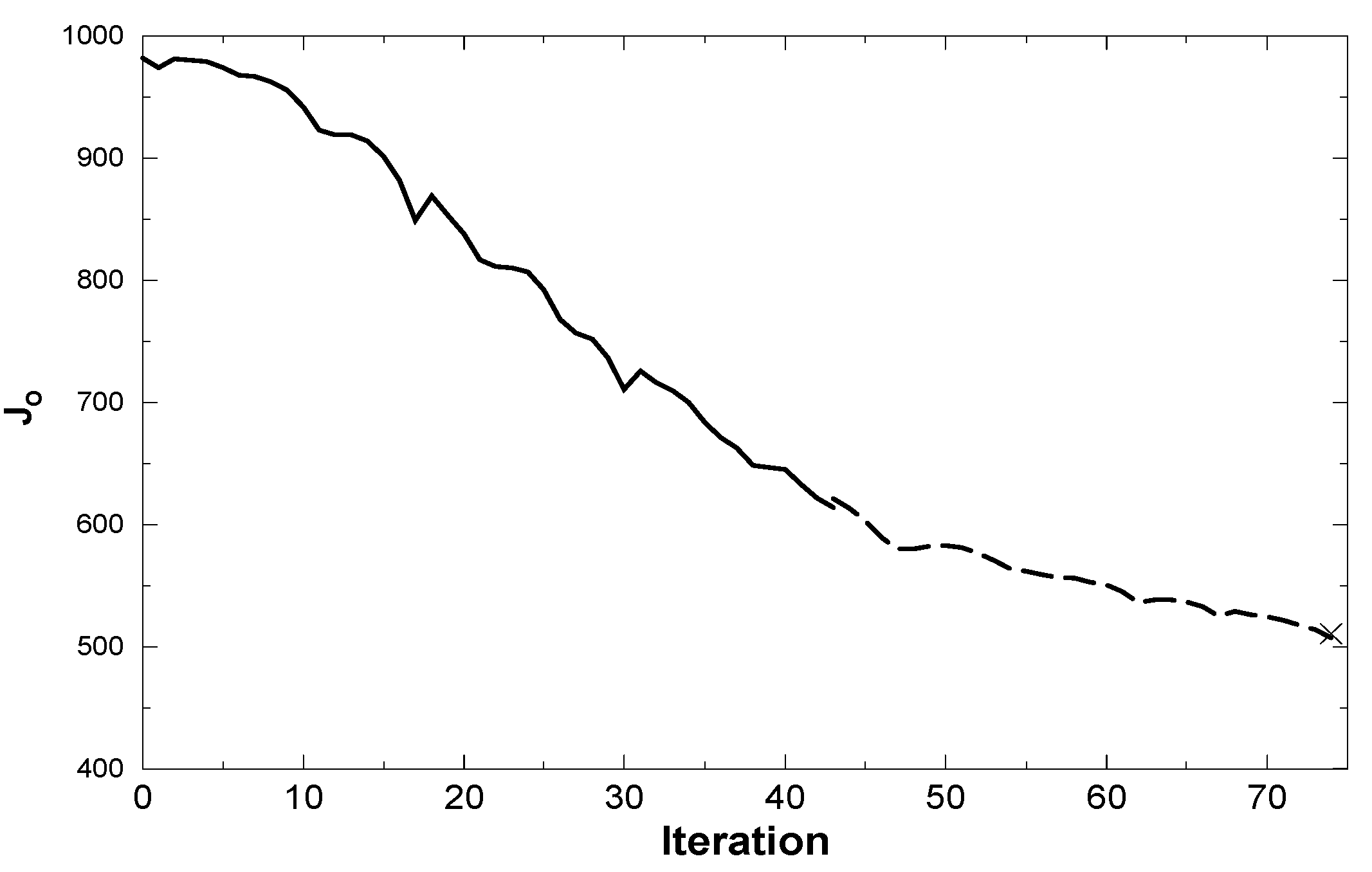
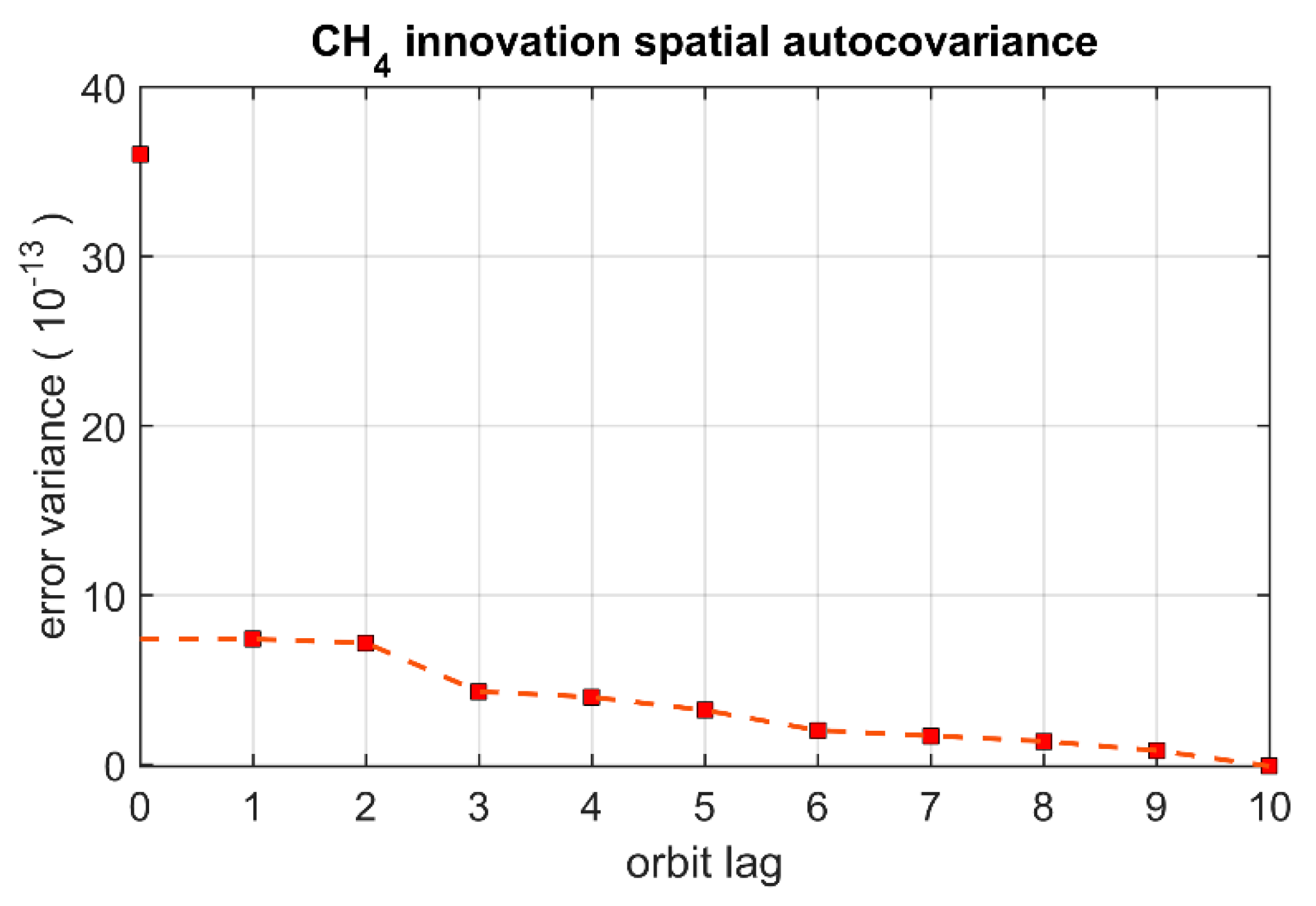
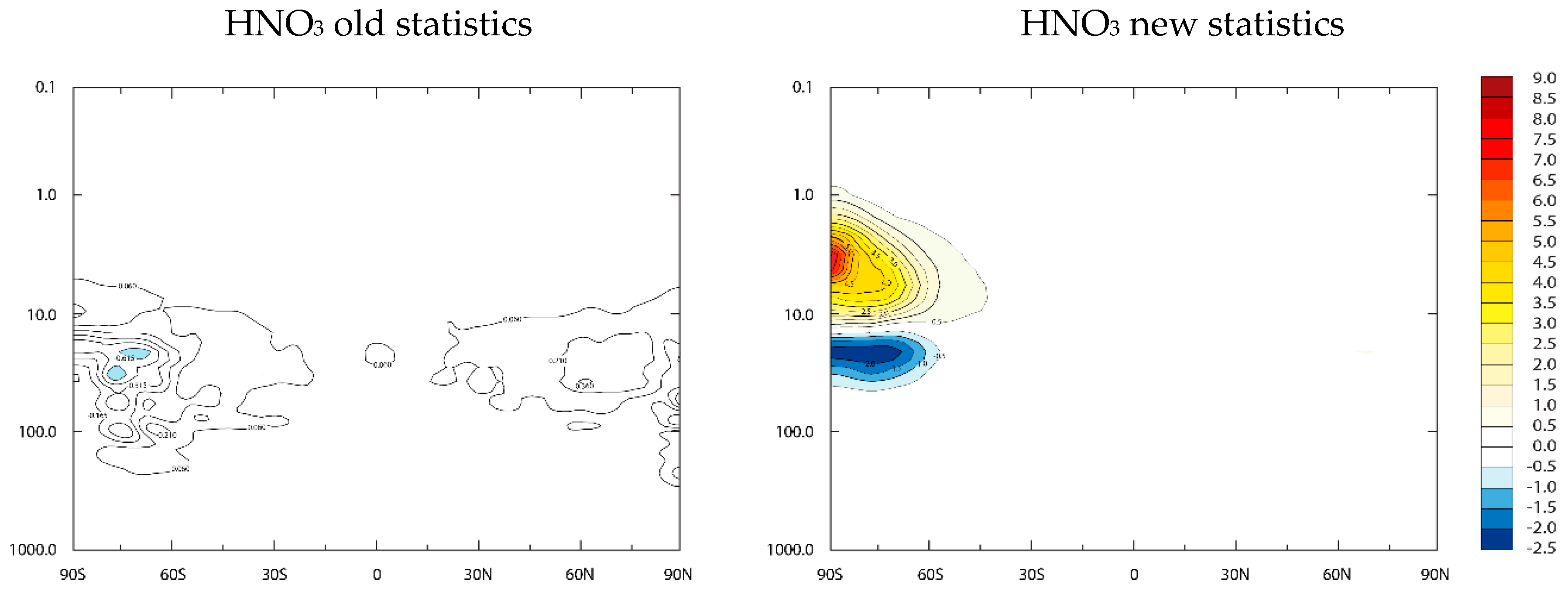
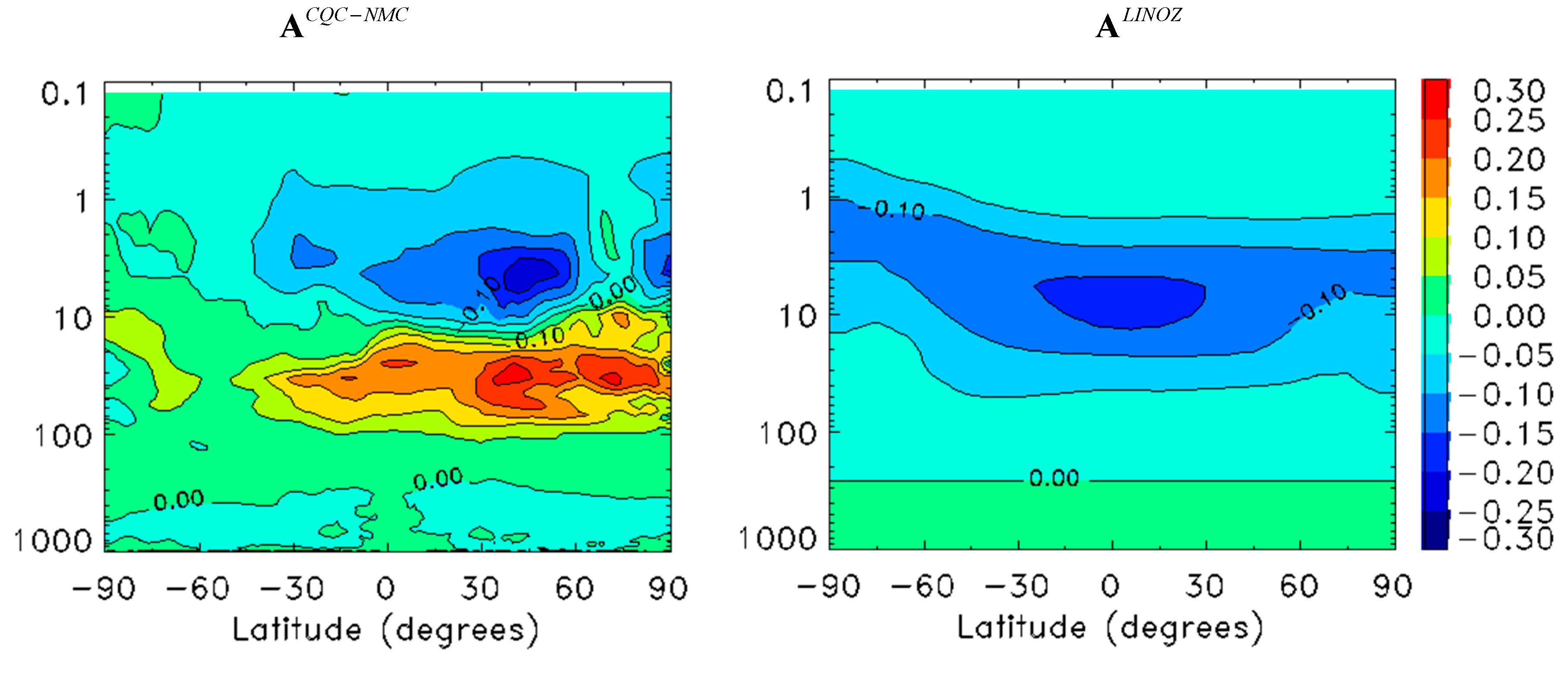
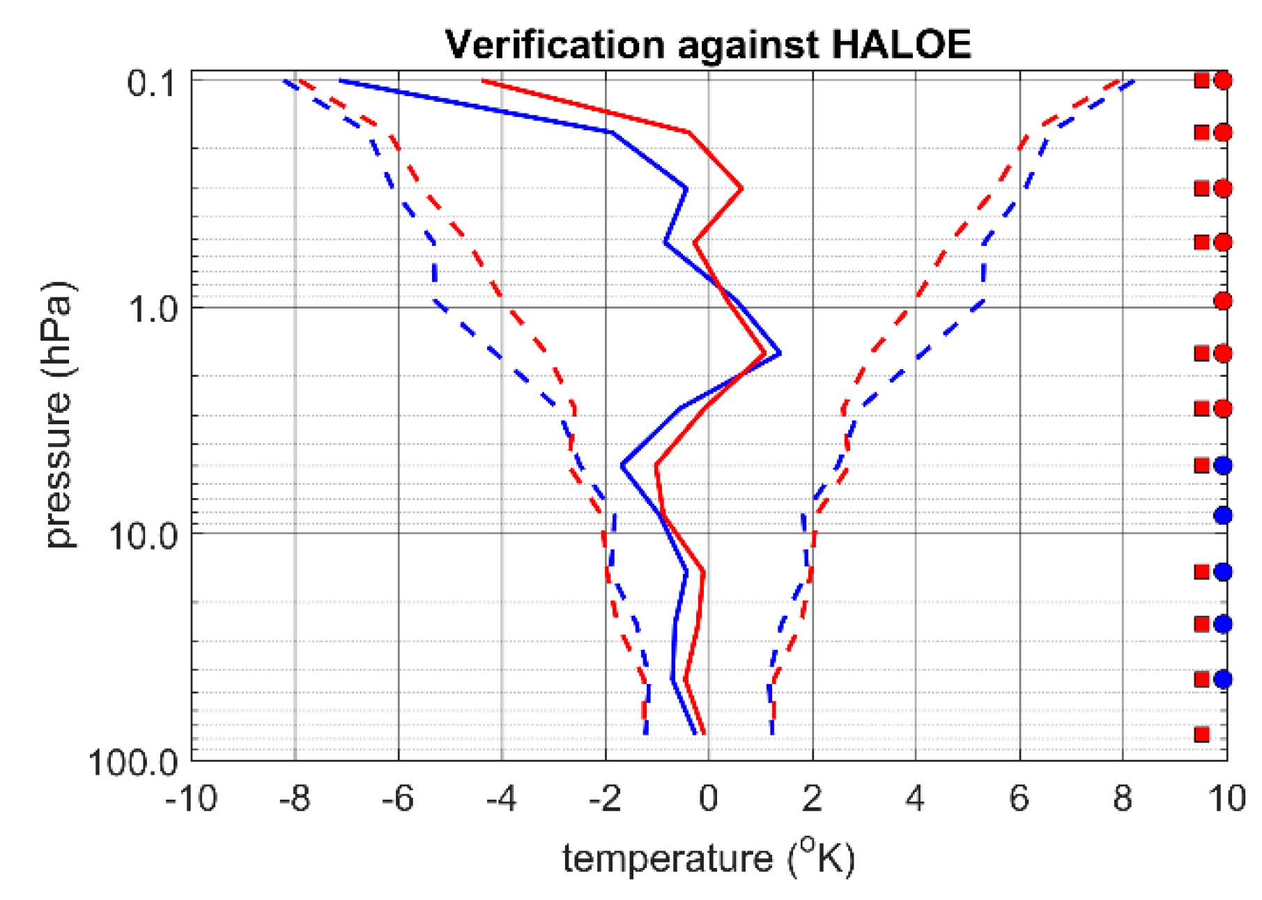
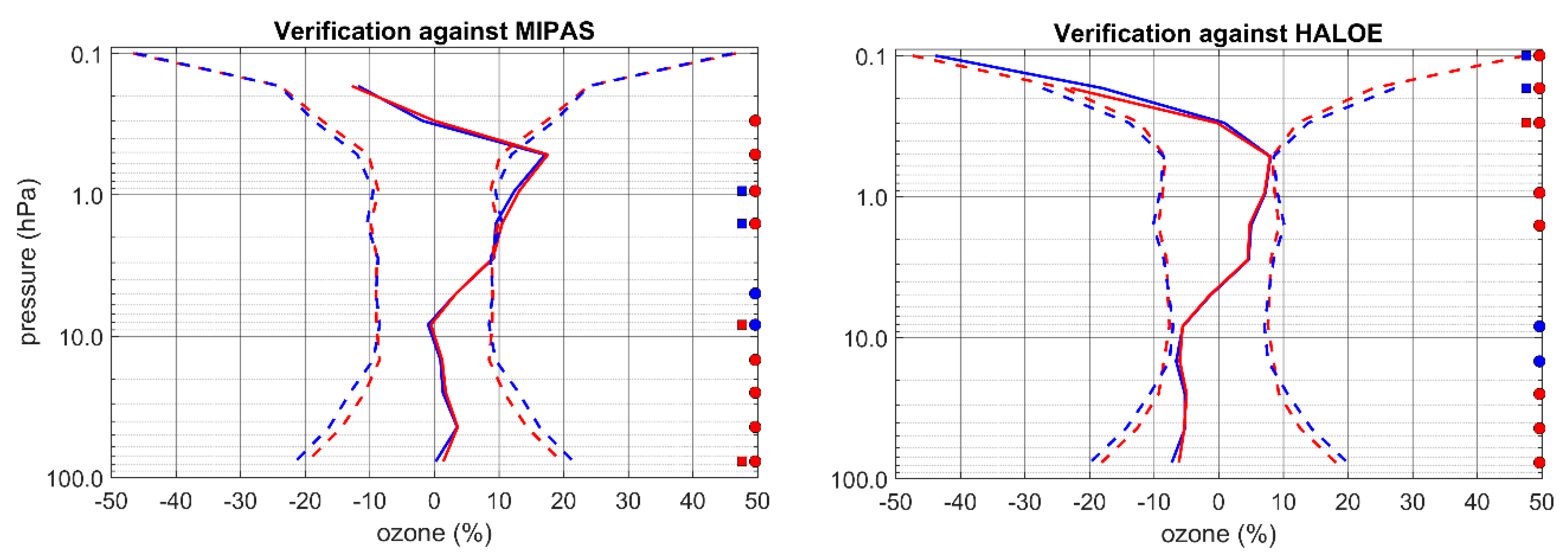
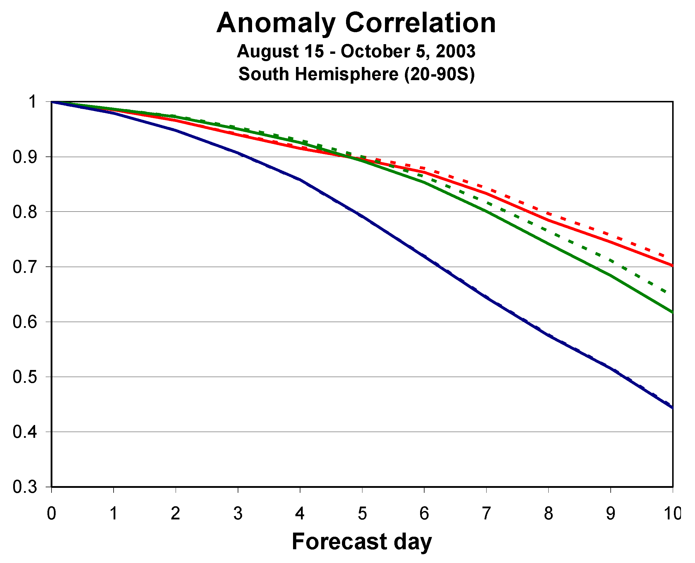
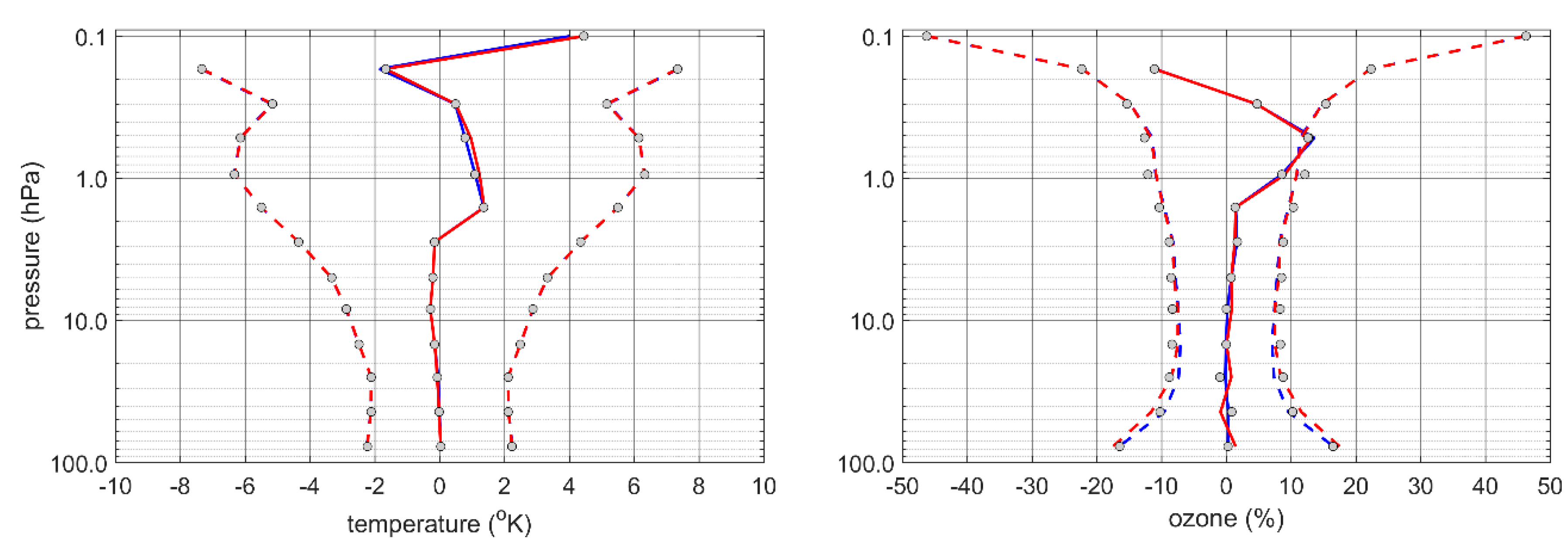
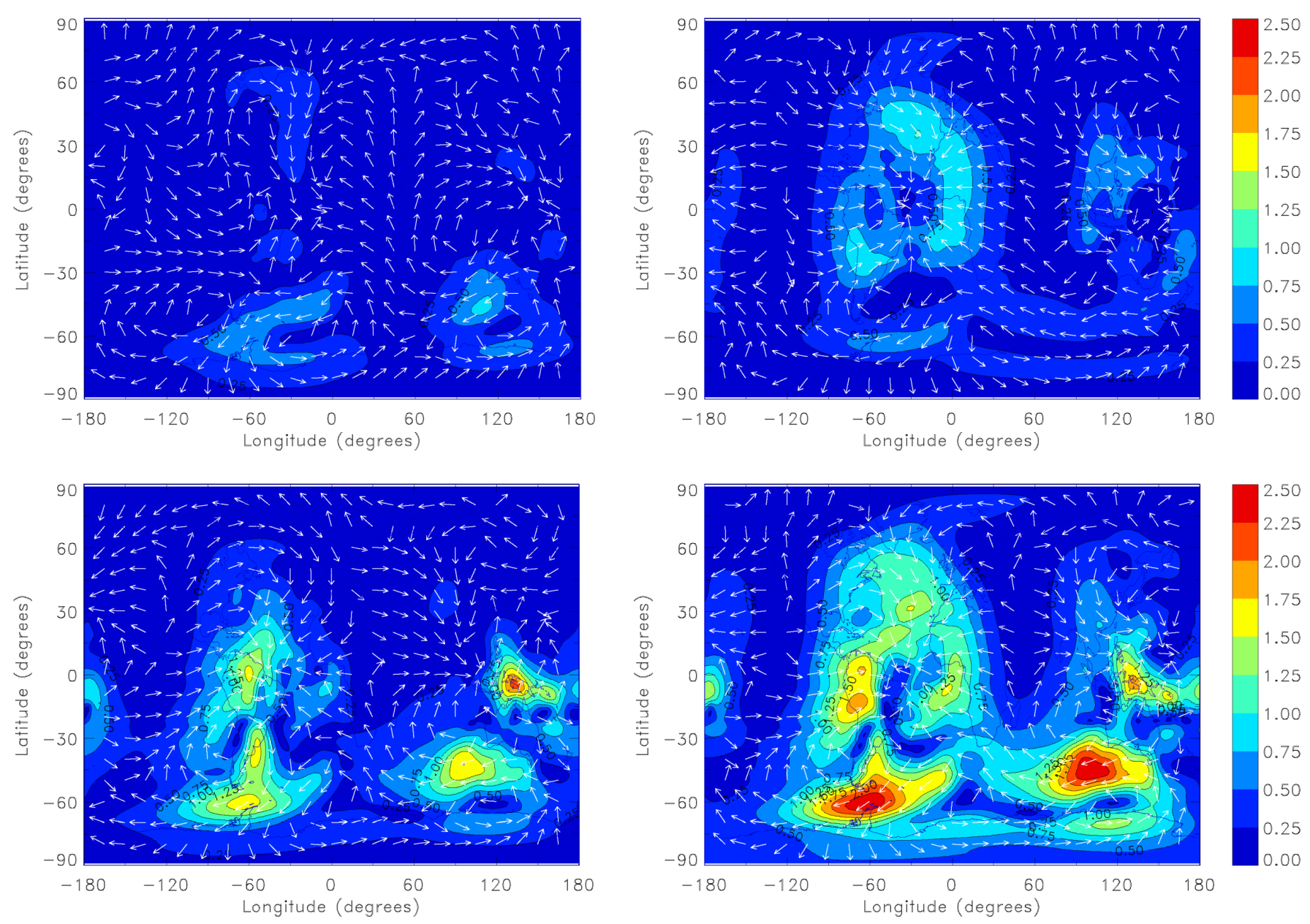
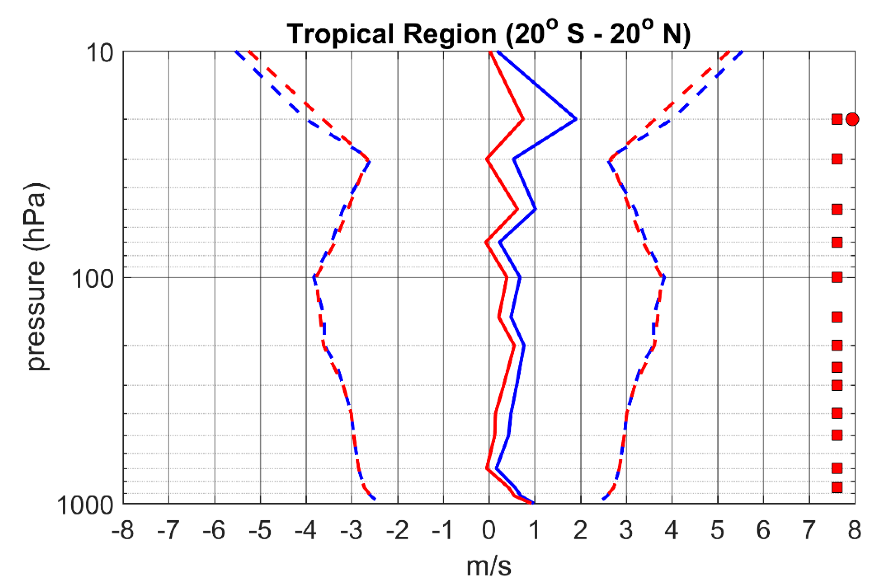
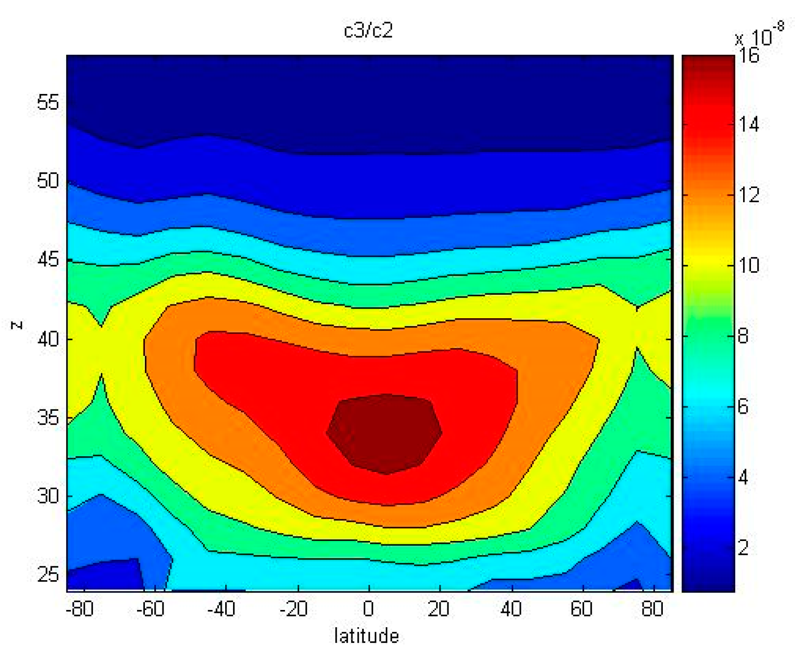