Article

April Vegetation Dynamics and Forest–Climate Interactions in Central Appalachia

1
School of Geosciences, University of South Florida, Tampa, FL 33620, USA
2
Department of Geology and Geography, West Virginia University, Morgantown, WV 26506, USA
3
Department of Geography, Kyung Hee University, Seoul 02447, Korea
*
Author to whom correspondence should be addressed.
Atmosphere 2019, 10(12), 765; https://doi.org/10.3390/atmos10120765
Submission received: 28 October 2019 / Revised: 26 November 2019 / Accepted: 28 November 2019 / Published: 2 December 2019

Abstract

:
The study of land–atmosphere (L–A) interactions is an emerging field in which the effects of the land on the atmosphere are strongly considered. Though this coupled approach is becoming more popular in atmospheric research, L–A interactions are not fully understood, especially in temperate regions. This study provides the first in-depth investigation of L–A interactions and their impacts on near-surface climate conditions in the Appalachian region of the Eastern United States. By way of statistical analysis, we explore vegetation dynamics, L–A interactions, and the consequences for near-surface climate, along with the competing effects of the albedo (energy) and moisture (evapotranspiration and soil moisture) feedback. Based on the results from linear regression, composite, and correlation analyses, we conclude that: (1) a statistically significant increasing trend in April vegetation exists from 1982 to 2015 in central Appalachia; (2) there was empirical evidence that this increasing vegetation trend was significant and altered near-surface climatic conditions, as indicated by significantly enhanced latent heat flux, 2 m-specific humidity, and soil moisture; and (3) the dominant biogeophysical process responsible for the changes in near-surface climate conditions could be the positive moisture feedback process.

1. Introduction

The Appalachian region follows the spine of the Appalachian Mountain chain and includes the surrounding dissected plateaus located in the eastern United States (Figure 1). This region is home to dense forests, scenic mountains, and freshwater streams, altogether covering more than 200,000 square miles in total surface area [1]. An estimated 24.8 million people live in cities and rural communities in Appalachia. The region’s natural landscape and its resources hold significant cultural and economic value for its residents [2]. The forests of Appalachia provide a wide range of ecosystem goods and services to the region, including wildlife habitats, watershed services, wood products, soil erosion prevention, recreation, tourism, and cultural services [1]. Considering the cultural and economic importance of natural resources in the region, an investigation of the biogeophysical processes that promote healthy vegetation growth in Appalachia is critical, especially with a changing climate and land use practices that could disrupt the balance of forest health [3,4].
The history of land use and land cover change (LULCC) in the Appalachian region began in the 1800s with the clearing of forests for agricultural practices [6]. By the mid 1800s, the agricultural lands were largely abandoned, and a period of forest regeneration was initiated [6]. Steyaert and Knox [6] remarked that the forest regeneration period was followed by extensive logging operations in the late 1800s and early 1900s. Along with logging, coal mining has been a common method of resource extraction throughout the history of the Appalachian region. Though surface coal mining has existed in the region since the 1800s, there has been a significant increase in activity since the 1970s [7].
In more recent years, surface mining and the reclamation of abandoned mines have driven LULCCs in the region [7,8]. The mountaintop removal and valley fill surface mining processes involve the removal of surface vegetation, the explosion of the overlying rock layers, the mining of the actual coal beds, and the placement of overburden material into surrounding valleys [9]. This mining process significantly changes the natural vegetation, surface topography, and subsurface structure of the landscape [7,9]. The central Appalachian subregion (Figure 1), which includes portions of West Virginia, Kentucky, Virginia, and Tennessee, has experienced intense LULCCs due to surface mining and mine reclamation processes. Pericak et al. [7] calculated a total surface mining footprint of 5900 km2 in central Appalachia, with 2900 km2 of that footprint resulting from mining operations during the period of 1985–2015. Given the recent and historical LULCCs in central Appalachia, this geographical region provides a unique opportunity to study the impacts of land surface dynamics on the near-surface atmosphere through the lens of land–atmosphere (L–A) interactions.
The more common perspective on the associations between the land and atmosphere is that atmospheric processes influence both land surface characteristics and land surface dynamics. In other words, the usual thought is that climate influences the biogeophysical characteristics in a given region. Thus, considerations regarding how these L–A interactions influence climate patterns has traditionally been limited. While climatic conditions influence the biosphere and land surface, a relatively newer perspective considers the ways in which the land and its biogeophysical characteristics affect climate [10]. The roles of L–A interactions in climate are usually observed at the local and regional scale; however, perturbed L–A interactions have the ability to significantly alter large-scale climate patterns [11,12]. These L–A interactions are under further investigation by using modeling analysis and observational evidence. Furthermore, the perspective of how L–A interactions affect climate patterns is being integrated into the approach to understanding various phenomena in climate science [13].
Land surface characteristics, like surface albedo, roughness, and wetness—which are all related to soil and vegetation properties—can affect near-surface climate conditions through energy, momentum, and moisture exchanges between the Earth’s surface and the atmosphere [10,14]. Initial alterations to the land surface characteristics may amplify the climatic impacts of land surfaces through positive feedback in L–A interactions [3,10,14]. The disturbed conditions could be associated with human-induced land use and land cover changes, including urbanization, agriculture land-use, and deforestation/afforestation, while some may be a result of natural phenomena, like wildfires and extreme climatic events such as heatwaves, droughts, and floods [15,16]. The primary processes of L–A interactions that influence climate are changes in the albedo and the partitioning of radiation into sensible and latent heat fluxes (e.g., [11,14]). A shift in the albedo and turbulent heat flux regimes due to LULCCs can disturb associated feedback mechanisms, leading to an even more pronounced change in the energy, momentum, and moisture budget of the region [3,4].
The two key biogeophysical processes that influence interactions between the land and the atmosphere are energy feedback (e.g., albedo) and moisture (e.g., evapotranspiration and soil moisture) [17]. Charney [18] first identified the albedo feedback in the Sahel region of Africa and suggested that this mechanism could be a factor in initiating and prolonging drought conditions. A shift in albedo, the proportion of incident radiation reflected by a surface, may change energy and surface moisture balances due to modifications in latent heat flux (LE) and atmospheric moisture flux convergence [10,19]. Vegetated surfaces have a lower albedo than surfaces with bare soil or low vegetation because they absorb more incident radiation [18,20]. Vegetation loss results in a greater albedo and less energy available for transfer to the lower atmosphere through LE and moisture flux convergence [20]. The increased albedo disrupts the balance between sensible heat flux (H) and LE, two ways in which the surface cools itself [10]. For example, the high albedo of the Sahel region leads to a net loss of radiative heat near the land surface, initiating a circulation pattern of descending air [18]. Moreover, this descending air and adiabatic heating can result in drier and warmer conditions that are less favorable for vegetation growth [10,18]. An initial reduction of vegetation cover paired with human-induced LULCCs (e.g., deforestation or land degradation) further increases the albedo, leading to a decrease in precipitation, exacerbating the dry conditions and reducing vegetation to a greater extent through this positive feedback [10,18,19].
The moisture feedback has been investigated and confirmed by a number of studies (e.g., [21,22]). An increase in soil moisture can be linked to an increase in vegetation cover and thus an increase in atmospheric moisture through evapotranspiration (ET) (e.g., [23]). Greater quantities of available atmospheric moisture may then lead to cloud formation and increased rainfall, though this is not always certain due to the complex dynamics involved with precipitation [17,23]. This increased rainfall can enhance soil moisture and create more favorable conditions for enhanced vegetation growth, thus leading to more ET through this positive moisture feedback mechanism [17,24]. On the other hand, a significant increase in soil moisture and ET also affects energy feedback through a cooling effect that is caused by the partitioning of radiative heat flux into primarily latent heat [17,25]. A recent study demonstrated that while the positive soil moisture–precipitation feedback is predominant over the land surface, a non-negligible negative feedback may occur over dry and wet regions [26]. In other words, preexisting environmental conditions may influence the direction (positive or negative) and overall impact of the soil moisture–precipitation feedback.
Though these two biogeophysical processes have been investigated and confirmed, they differ by region and with vegetation types. The net radiative forcing of a given region can be influenced by whichever feedback is dominant there. Bonan [11] offered a review of the dominant forcing and feedback of three different biomes with distinct vegetation types: tropical forests, boreal forests, and temperate forests. Most tropical forests have a negative radiative forcing, or cooling effect, and increase precipitation through high rates of ET and the dominant moisture feedback (e.g., [27]). On the other hand, boreal forests may have a positive radiative forcing, or warming effect, because of the associated low surface albedo that leads to the absorption of radiation [11]. Lastly, the net forcing of temperate forests is unknown because the albedo and moisture feedback often compete and may cancel each other out [11].
As noted in Bonan’s [11] review, the dominant biogeophysical mechanism and net radiative forcing for temperate forests is currently undecided. In the summer, the moisture feedback is usually dominant, leading to cooler and wetter conditions [28]. Conversely, the albedo feedback has a greater influence in the winter, with a lower albedo resulting in radiation absorption and a positive radiative forcing [28]. The Appalachian region is predominantly covered with temperate forests; thus, the L–A interactions between Appalachian forests and the atmosphere may influence the near-surface climate conditions through the two competing biogeophysical processes of energy and moisture feedback. In this study, we investigated vegetation dynamics, these competing biogeophysical processes, and their impacts on near-surface climate in central Appalachia by using statistical analysis.
There are no previous studies on L–A interactions in the Appalachian region. Therefore, this was the first study that particularly examined vegetation dynamics and their impact on L–A interactions in this region. A more comprehensive understanding of Appalachian vegetation and climate dynamics could be used to help predict future changes and the possible consequences for L–A interactions under changing land use and climate conditions. The primary objectives of this study were the following:
  • Determine if there is a trend in vegetation change in the Appalachian Mountains region and, if so, at what spatial scale.
  • Investigate whether the potential trend is significant and influences near-surface climate conditions.
  • Identify the dominant biogeophysical process that is responsible for the possible changes in the near-surface climate conditions.

2. Data and Methods

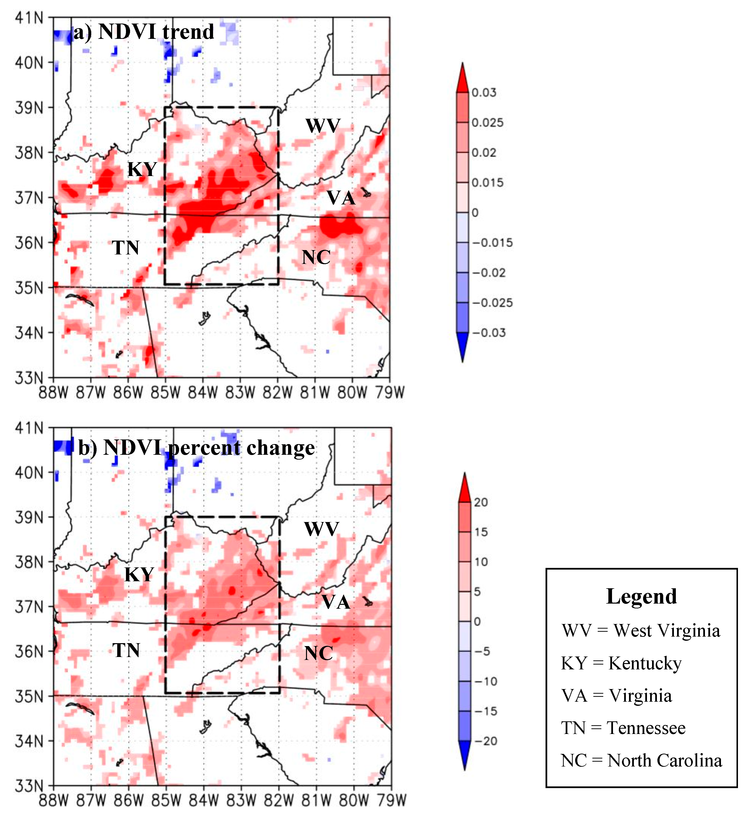
In order to identify trends in vegetation for the Appalachian region and investigate how they might impact local climate conditions, we first performed linear regression analysis of the normalized difference vegetation index (NDVI). The NDVI was selected as an indicator for vegetation changes in the region, and the method of linear regression was used to identify the trend in vegetation change for the study period 1982–2015. The statistically insignificant grid points were masked out at the 10% significance level to show only the statistically significant vegetation changes. We then extracted the April NDVI values over the central Appalachian region. The month of April was chosen for the NDVI extraction because it experienced the most significant trend in vegetation change within central Appalachia (outlined as the dotted rectangle in Figure 2). The extracted April NDVI values were detrended to remove the distortion from the underlying increasing trend that might have been linked to the secular warming trend.
We proceeded to conduct a composite difference analysis for the soil moisture, sensible heat flux (H), latent heat flux (LE), and 2 m-specific humidity variables. These variables were selected to investigate the possible influence of vegetation change on local moisture and energy. The composite analysis was performed to find the difference in each variable between years of high and low NDVIs in attempt to isolate the effects that vegetation change had on moisture and energy conditions. We followed with a correlation analysis between the NDVI and LE, H, 2 m-specific humidity, and soil moisture to examine the relationship between vegetation and each dependent variable. We sought to confirm the directional relationship observed in the composite analysis with the correlation analysis results.
Finally, we completed dryness index calculations using monthly mean precipitation (P) and potential evapotranspiration (PET) values to determine whether central Appalachia was water-limited or energy limited on an annual basis and for the month of April. The dryness index values were produced to help investigate which biogeophysical process might be dominant for the central Appalachian region based on energy and water limitations.

2.1. Data

We chose the NDVI, which is defined as the difference between near-infrared and red spectral reflectance normalized by their sum, as a vegetation indicator for this study [24,29]. Due to its strong correlation with photosynthetically active biomass, chlorophyll abundance, and energy absorption, this index has commonly been used as a vegetation greenness indicator [30]. Accordingly, the Normalized Difference Vegetation Index-3rd Generation (NDVI3g) time series dataset was used for the vegetation analysis. This NDVI dataset was derived from imagery collected by the Advanced Very-High-Resolution Radiometer (AVHRR) instrument included on the National Oceanic and Atmospheric Administration (NOAA) satellite series [31]. The dataset was obtained from the Global Inventory Modeling and Mapping Studies (GIMMS), which was made available by the Global Land Cover Facility at the University of Maryland. This NDVI3g dataset included bimonthly values for the time span of July 1981 to December 2015 at a grid increment of 0.08° (approximately 8 km).
The National Center for Environmental Prediction (NCEP) North American Regional Reanalysis (NARR) dataset was used for the land surface and near-land surface variables of soil moisture at 0–200 cm in depth, H and LE fluxes, and specific humidity at 2 m [32]. For turbulent heat fluxes, original values were multiplied by -1 at each grid point so that positive H and LE values represented energy transfers from land to atmosphere [33]. This dataset was constructed using the NCEP Eta model and its data assimilation system [32]. The NARR provided a long-term dataset for soil moisture, H, LE, and specific humidity beginning in 1979 over the spatial domain of North America. The monthly values were used for our analyses. The horizontal grid increment for this dataset was approximately 0.3° (approximately 32 km) and included 45 vertical layers.
Additionally, the gridded surface meteorological (GridMET) dataset was used for precipitation analysis. The GridMET dataset was created by combining temporal attributes from the North American Land Data Assimilation System Phase 2 (NLDAS-2) and spatial attributes from the Parameter-elevation Regressions on Independent Slopes Model (PRISM), which was done to optimize both temporal and spatial resolutions [34]. The GridMET dataset contained high-resolution gridded surface data over the continental United States beginning in 1979. The spatial grid increment was 1/24th° (approximately 4 km), and the data were updated daily for precipitation. We used the monthly average for total precipitation in our precipitation analysis.
Finally, we used Climate Research Unit (CRU) monthly mean P and PET data for dryness index (DI) calculation as the ratio of long-term PET to P (PET/P). The DI was calculated at each grid point by using the averaged PET and P over thirty-four years of the study period (1982–2015). Grid points with DI > 1 were considered water-limited, and those with DI < 1 were considered energy limited [35]. The CRU P and PET high-resolution gridded data (CRU Time-series version 4.02) were compiled using observational meteorological stations over the global land surface [36]. This CRU dataset was available for the time period 1901–2017 at a 0.5° (approximately 50 km) grid increment.

2.2. Methods

2.2.1. Linear Regression Analysis

A linear regression analysis of the NDVI was used to determine if there was a change in vegetation by examining the spatial and temporal trends of vegetation cover in the Appalachian region during the study period 1982–2015. The regression coefficient parameters were estimated using the ordinary least squares method. The slope of the regression line, b, explained how the dependent variable (Y) changed over time (X) [37]. The NDVI was the dependent variable; thus, the slope explained how vegetation changed over time. We conducted a significance test for the linear regression coefficient to quantify significant vegetation changes, with a rejection of the null hypothesis with the slope equal to zero at the 10% significance level. We then masked out the statistically insignificant grid points, leaving only the grid points with statistically significant vegetation changes in the results. We also calculated an NDVI percent to the mean value at each grid point, which represented the NDVI change in percent in comparison to the April mean for the thirty-four years of 1982–2015. Finally, the statistically significant values from the NDVI time series were extracted at each grid point over the domain with the geographic extent of 35° N to 39° N and 82° W to 85° W (shown as the dotted rectangle in Figure 2a) to be used for the detrended composite analysis.

2.2.2. Detrended Composite Analysis

A detrended composite analysis was utilized to determine whether or not the changes in H and LE fluxes, 2 m-specific humidity, soil moisture, and precipitation were associated with significant vegetation changes in the Appalachian region. April was identified as the month with the strongest changes of the NDVI in the central Appalachian region over the period 1982–2015 (Supplementary Figure S1), so the analysis for land surface and atmospheric variables was conducted for April. First, the extracted NDVI time series was used to calculate the slope coefficient for the NDVI regression line, which was estimated by the ordinary least squares method. Second, the time-weighted slope value was removed from the original value of the variable in order to remove the trend. The detrended values were then used to identify the nine years of the highest April NDVI (i.e., top 26.5% of the observations; n = 34, 1982–2015) and nine years of the lowest April NDVI (i.e., bottom 26.5%) in the central Appalachian region. We proceeded to calculate the composite differences of the moisture and energy variables between the nine years (1990, 1991, 1992, 1994, 1995, 2003, 2005, 2010, and 2012) of the highest April NDVI and the nine years (1983, 1984, 1993, 1996, 2007, 2008, 2009, 2014, and 2015) of the lowest April NDVI. Subsequently, a t-test for a two sample difference of means [38] was performed to quantify the significant differences for the composite analysis of each variable, with a rejection of null hypothesis with zero difference between the means of two variables at the 10% significance level. Lastly, the statistically significant regions at the 10% significance level were contoured on each map.

2.2.3. Detrended Correlation Analysis

We used a detrended correlation analysis to evaluate the relationship between vegetation and H and LE fluxes, 2 m-specific humidity, soil moisture, and precipitation. The same process for detrending in the composite analysis was used for this analysis. First, the slope coefficient for each variable was calculated by using ordinary least squares regression. Second, we extracted the slope value, weighted by time, from the original variable value. These detrended variables were utilized in the correlation analysis with the NDVI time series. Pearson’s correlation coefficient (r-value) was calculated at each grid point for all land surface and atmospheric variables to evaluate the strength and direction of relationship with vegetation, with significant regions contoured at the 10% significance level for each map. The detrended correlation results were compared with the spatial patterns of these variables from the detrended composite results. We estimated the association between the NDVI and the climate variables using the time series of the NDVI and each variable extracted over the study region of central Appalachia.

3. Results

3.1. NDVI Trends

Based on the linear regression analysis of the NDVI trends for each separate month from 1982 to 2015 (Supplementary Figure S1), the month of April experienced the most statistically significant vegetation changes in the central Appalachian region, which are shown in Figure 2. These statistically significant changes of the April NDVI occurred primarily near the central Appalachian area (eastern Kentucky, southwestern West Virginia, southwestern Virginia, eastern Tennessee, and western North Carolina), which was identified as the domain of interest in this study. The average increase in the NDVI in this region was approximately 0.02–0.04 per decade (Figure 2a), which represented an increase in the NDVI by 10–20% for the thirty-four years of 1982–2015 (Figure 2b).

3.2. Detrended Composite Difference Analysis

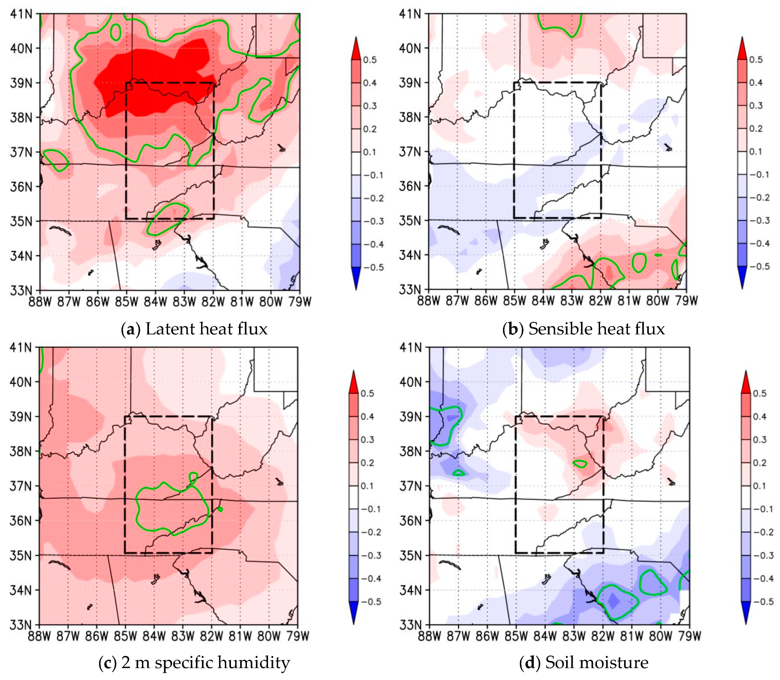
The detrended composite analysis results showed a statistically significant increasing LE spatial pattern that ranged from 6 to 12 W/m2 over central and south central Appalachia, which is indicated by the contoured region of statistical significance on the map (Figure 3a). There was a corresponding decreasing pattern (1–9 W/m2) in H around the same region, though this pattern was less statistically significant in extent and magnitude (Figure 3b). Additionally, there was a statistically significant increase in 2 m-specific humidity that ranged from 0.2 to 0.8 g/kg over central and south central Appalachia (Figure 3c). Finally, the detrended composite results for soil moisture of 0–200 cm in depth displayed a statistically significant increase in central Appalachia that ranged from 60 to 80 kg/m2 (Figure 3d). The spatial pattern for increasing soil moisture extended into south central Appalachia, but the increase was not statistically significant there (Figure 3d).

3.3. Detrended Correlation Analysis

The detrended correlation analysis results indicated a statistically significant positive correlation between the NDVI and LE, with an r-value that ranged from 0.3 to 0.5 over central Appalachia (Figure 4a). The results showed another statistically significant positive correlation between the NDVI and LE in south central Appalachia (western North Carolina) with an r-value range of 0.3–0.5 (Figure 4a). Though statistically insignificant, the spatial pattern from the detrended correlation analysis for H (Figure 4b) was generally consistent with the detrended composite results for H (Figure 3b). Thus, the negative correlation between the NDVI and H (Figure 4b) supported the detrended composite analysis results for H (Figure 3b), which indicated a pattern of lower H with an increasing NDVI. The detrended correlation analysis results displayed a statistically significant positive correlation between the NDVI and 2 m-specific humidity around south central Appalachia with an r-value that ranged from 0.3 to 0.4 (Figure 4c). Again, the statistically significant positive correlation pattern from the detrended correlation analysis results (Figure 4c) upheld the detrended composite analysis results for the 2 m-specific humidity (Figure 3c), which indicated a pattern of greater specific humidity with an increasing NDVI. Lastly, the detrended correlation results depicted a small area in central Appalachia with a statistically significant positive correlation, with an r-value of 0.3–0.4, between the NDVI and soil moisture at 0–200 cm in depth (Figure 4d). The sign of the correlation (+) and spatial pattern of the detrended correlation analysis results (Figure 4d) confirmed the results from the detrended composite analysis for soil moisture (Figure 3d), which indicated a pattern of increasing soil moisture with an increasing NDVI. Additionally, the detrended correlation between the time series of the NDVI and climate variables, extracted over the study region, supported significant positive associations of the NDVI with LE (r = 0.44; p-value = 0.01) and 2 m-specific humidity (r = 0.33; p-value = 0.05). The direction of the relationships of the NDVI with H (r = −0.07) and soil moisture (r = 0.12) was consistent with the spatial patterns in Figure 4b,d, respectively, but the correlations were not statistically significant.

3.4. Dryness Index Analysis

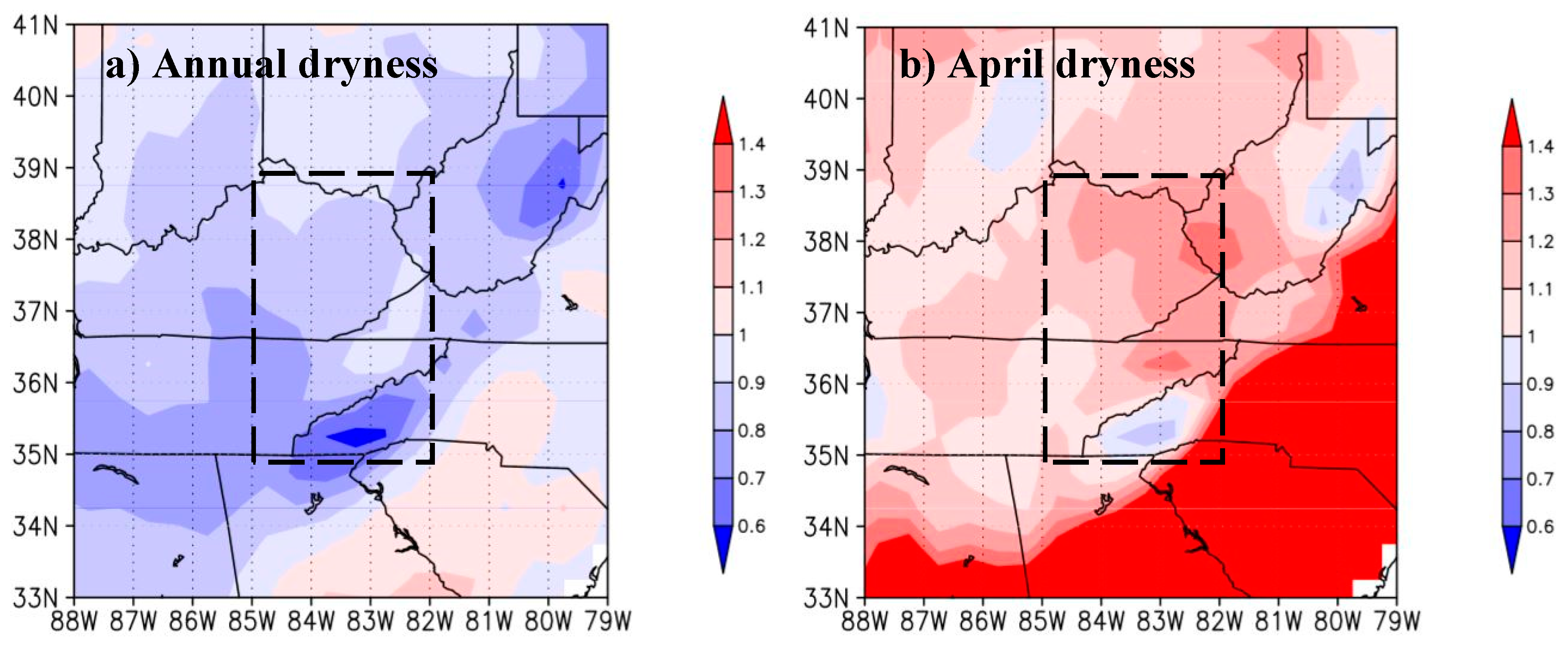
The DI calculations indicated that the Appalachian region was energy limited on an annual basis, which was shown by a DI value less than 1 in most of the region (Figure 5a). The DI value was less than 1, so P > PET, signifying a surplus of precipitation and a limitation of energy sources. In April, however, the DI values were greater than 1 in the Appalachian region, except for higher altitude regions in southern and central Appalachia. Overall, these results indicated that the Appalachian region was water-limited during the mid-spring month, April (Figure 5b). In this case, PET > P, so the demand for moisture was greater than what was provided through precipitation in this region during April. In other words, there was a moisture deficit (or energy surplus) during April. Interestingly, the border region of West Virginia and Kentucky exhibited an even greater moisture deficit (DI > 1.3), which was the same region where significant changes in surface and atmospheric variables were identified with an increasing April NDVI (see Figure 3a,d).

4. Discussion and Conclusions

The linear regression analysis results for vegetation demonstrated an increasing trend of 0.02–0.04 per decade, which represented a 10–20% increase in the April NDVI in the central Appalachian region from 1982 to 2015. This trend could have been a result of spring phenology dynamics. Yue et al. [39] documented how deciduous forests in the eastern United States have experienced phenological changes. According to Yue et al. [39], the trend for the start of season (SOS) from 1982 to 2011 was between −0.5 and −0.4 day/year. At this rate, the SOS dates advanced approximately 11.6–14.5 days from April 21st to May 14th to April 10th–30th [39]. Similarly, White et al. [40] (Figure 14) discovered a statistically significant earlier SOS trend in central Appalachia from 1982 to 2006 using the harmonic analyses of NDVI time-series–fast Fourier transform (HANTS-FFT) and midpoint pixel methods in their phenology models, providing more evidence for the earlier SOS trend in central Appalachia. This earlier growing season, which is almost certainly related to secular warming, could be the cause of the significantly increasing April NDVI trend identified in our results. Moreover, this long term shift in spring phenology may impact surface water and energy balances [41].
The patterns of land surface and atmospheric variables identified from detrended composite and correlation analyses suggested that the moisture feedback process could be the dominant biogeophysical process in the central Appalachian region for April. Our results displayed an increase in LE, a decrease in H, an increase in 2 m-specific humidity, and an increase in soil moisture at 0–200 cm in depth for April (Figure 3a–d). These variables have previously been identified to play an important role in the moisture feedback process [17]. Additionally, the lower magnitude of change in H (decrease ranging from 1–9 W/m2), compared to LE (increase ranging from 6–12 W/m2), could be explained by an increase of incoming radiation due to decreasing albedo, which compensates the reduced H fluxes due to increasing vegetation (e.g., [11]). The detrended composite and correlation results were generally consistent in regards to the direction and magnitude of the associations between vegetation and climate variables. The spatial patterns of detrended composite and correlation results were also consistent with the spatial pattern of increasing April vegetation. Therefore, the increasing April vegetation could be linked to the changes in land surface and climatic variables through L–A interactions. The changes in climatic conditions in the surrounding regions might be associated with the changes in the NDVI over the regions which have a similar year-to-year variability of the NDVI over the study region. In order to isolate the effects of the NDVI over the surrounding regions, an idealized simulation that uses a coupled land–atmosphere climate model is required.
The dryness index calculations, which were used to help identify the dominant biogeophysical mechanism, indicated that the Appalachian region was water-limited in April, except for the higher altitude regions in south central and central Appalachia. These higher altitude regions receive more moisture, and their land surface is covered with dense forests. Eastern West Virginia contains the Monongahela National Forest, which ranges from 1000 feet (301 m) to 4863 feet (1482 m) in elevation above sea level [42]. Western North Carolina is home to the Nantahala National Forest, where elevations reach 5800 feet (1768 m) [43]. The high altitudes in these locations lead to a more pronounced orographic precipitation effect, which could likely be the cause of this annual mean energy deficit (or moisture surplus), indicated by the DI values (DI < 1) in Figure 5a. The orographic precipitation effect also explains the significant water-limited region highlighted in red in Figure 5b. The descending air on the leeward (eastern) side of the Appalachian Mountains loses moisture from the precipitation caused by orographic lift on the windward (western) side, creating a rain-shadow effect in which dryer conditions dominate the landscape. In theory, the moisture feedback process is dominant in conditions that are water-limited [21]. Thus, the widespread water-limited results of the DI analysis (Figure 5b) supported that the moisture feedback process is dominant in the central Appalachian region for April.
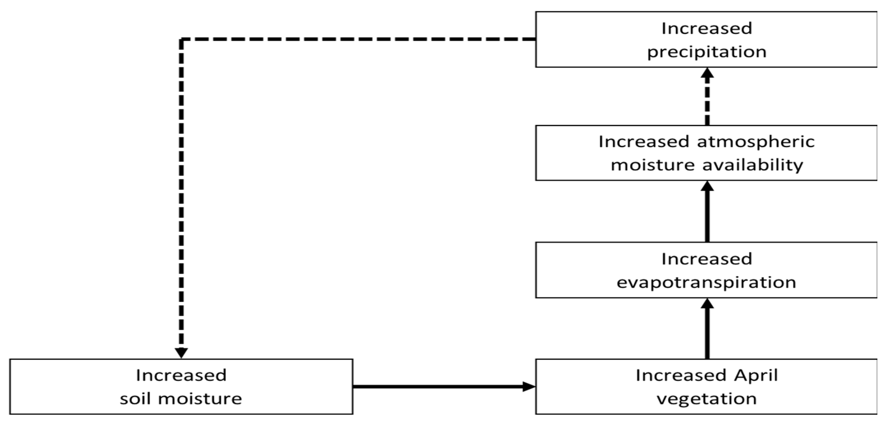
The schematic diagram that we developed, depicted the proposed moisture process and potential feedback mechanism for L–A interactions in central Appalachia (Figure 6). This process began with the increased April vegetation pattern, which was based on the NDVI regression analysis results. The increased vegetation was linked to an increase in latent heat fluxes and 2 m-specific humidity based on the detrended composite and correlation analysis results. The increase in LE, the corresponding decrease in H, and the greater specific humidity may have enhanced atmospheric moisture availability through the exchange of moisture and energy from the Earth’s surface to the atmosphere via evapotranspiration. Next, based on the anomaly in the precipitation pattern shown in the results of the composite analysis of precipitation, it can be suggested that the enhanced atmospheric moisture availability could be providing favorable conditions for cloud formation and possibly an increase in precipitation (Supplementary Figure S2). Lastly, greater precipitation in the region could result in increased soil moisture, which may then lead to more favorable soil conditions for further vegetation growth. After the enhanced vegetation growth, the cycle may continue and result in even greater atmospheric moisture conditions and L–A interactions, which is a positive feedback of vegetation and precipitation.
In summary, we addressed the three primary research objectives outlined in the introduction. These objectives were:
  • Determine if there is a trend in vegetation change in the Appalachian Mountains region and, if so, at what spatial scale.
  • Investigate whether the potential trend is significant and influences near-surface climate conditions.
  • Identify the dominant biogeophysical process that is responsible for the possible changes in the near-surface climate conditions.
After our analysis and consideration of the results, we concluded that:
  • A statistically significant increasing trend in April vegetation existed from 1982 to 2015 in central Appalachia.
  • There was empirical evidence that this increasing vegetation trend was significant and altered near-surface climatic conditions.
  • We proposed that the dominant biogeophysical process responsible for the changes in near-surface climate conditions was the positive moisture feedback process.
Future work should focus on confirming this plausible biogeophysical process and feedback mechanism using a coupled land–atmosphere climate model simulation. Additionally, a more empirical approach is required to find the causal association between vegetation change and climate conditions in Appalachia. A causality test will aid in determining whether the vegetation change is altering climate conditions or whether the climate conditions are causing the increased vegetation. An increasing trend in the October and November NDVIs (Supplemental Figure S1) suggests a delay in fall seasonal NDVI reduction. Moving forward, we can investigate this trend more closely to evaluate the possible impacts of a later end-of-season on vegetation–climate interactions in the Appalachian region during fall. Furthermore, future work can focus on the influence of surface mining and mine reclamation on the local L–A interactions in central Appalachia. Finally, further investigation is needed for the possible impacts of the altered feedback between vegetation and climate on ecological, hydrological, and societal and human dimensions.

Supplementary Materials

The following are available online at https://www.mdpi.com/2073-4433/10/12/765/s1, Figure S1: Linear regression analysis of NDVI from 1982–2015 for all 12 months, starting with January (top, left) and February (top, right) then proceeding downwards. The dotted rectangle represents the domain of the study region, Figure S2: Detrended composite analysis of GridMET precipitation (mm/month) between 9 years of high/low NDVI. The dotted rectangle represents the domain of the study region.

Author Contributions

Conceptualization, E.L.; data curation, N.S. and E.L.; formal analysis, N.S. and E.L.; funding acquisition, N.S. and E.L.; investigation, N.S. and E.L.; methodology, E.L.; project administration, E.L.; resources, E.L.; software, E.L.; supervision, E.L.; validation, N.S. and E.L.; visualization, N.S and E.L.; writing–original draft, N.S. and E.L.; writing—review and editing, N.S. and E.L.

Acknowledgments

This study was supported in part by the West Virginia University Summer Undergraduate Research Experience (SURE) program. We thank Yaqian He of the Department of Geography at Dartmouth College for detailed comments and suggestions on spring phenology in the Eastern United States.

Conflicts of Interest

The authors declare no conflict of interest.

References

  1. ARC. An Assessment of Natural Assets in the Appalachian Region: Forest Resources. Available online: https://www.arc.gov/assets/research_reports/AssessmentofNaturalAssetsintheAppalachianRegion-ForestResources.pdf (accessed on 20 May 2019).
  2. Nesbitt, J.T.; Weiner, D. Conflicting environmental imaginaries and the politics of nature in Central Appalachia. Geoforum 2001, 32, 333–349. [Google Scholar] [CrossRef]
  3. Foley, J.A.; DeFries, R.; Asner, G.P.; Barford, C.; Bonan, G.; Carpenter, S.R.; Chapin, F.S.; Coe, M.T.; Daily, G.C.; Gibbs, H.K. Global consequences of land use. Science 2005, 309, 570–574. [Google Scholar] [CrossRef] [PubMed]
  4. Pielke, R.A. Land use and climate change. Science 2005, 310, 1625–1626. [Google Scholar] [CrossRef] [PubMed]
  5. Appalachian Regional Commission, Subregions in Appalachia. 2009. Available online: https://www.arc.gov/research/mapsofappalachia.asp?MAP_ID=31 (accessed on 1 September 2019).
  6. Steyaert, L.T.; Knox, R.G. Reconstructed historical land cover and biophysical parameters for studies of land-atmosphere interactions within the eastern United States. J. Geophys. Res. Atmos. 2008, 113. [Google Scholar] [CrossRef]
  7. Pericak, A.A.; Thomas, C.J.; Kroodsma, D.A.; Wasson, M.F.; Ross, M.R.; Clinton, N.E.; Campagna, D.J.; Franklin, Y.; Bernhardt, E.S.; Amos, J.F. Mapping the yearly extent of surface coal mining in Central Appalachia using Landsat and Google Earth Engine. PLoS ONE 2018, 13, e0197758. [Google Scholar] [CrossRef]
  8. Simmons, J.A.; Currie, W.S.; Eshleman, K.N.; Kuers, K.; Monteleone, S.; Negley, T.L.; Pohlad, B.R.; Thomas, C.L. Forest to reclaimed mine land use change leads to altered ecosystem structure and function. Ecol. Appl. 2008, 18, 104–118. [Google Scholar] [CrossRef]
  9. Ross, M.R.; McGlynn, B.L.; Bernhardt, E.S. Deep impact: Effects of mountaintop mining on surface topography, bedrock structure, and downstream waters. Environ. Sci. Technol. 2016, 50, 2064–2074. [Google Scholar] [CrossRef]
  10. Foley, J.A.; Costa, M.H.; Delire, C.; Ramankutty, N.; Snyder, P. Green surprise? How terrestrial ecosystems could affect earth’s climate. Front. Ecol. Environ. 2003, 1, 38–44. [Google Scholar]
  11. Bonan, G.B. Forests and Climate Change: Forcings, Feedbacks, and the Climate Benefits of Forests. Science 2008, 320, 1444–1449. [Google Scholar] [CrossRef]
  12. Chase, T.N.; Peilke, R.A., Sr.; Kittel, T.G.F.; Nemani, R.R.; Running, S.W. Simulated impacts of historical land cover changes on global climate in northern winter. Clim. Dyn. 2000, 16, 93–105. [Google Scholar] [CrossRef]
  13. Pielke, R.A.; Pitman, A.; Niyogi, D.; Mahmood, R.; Mcalpine, C.; Hossain, F.; Goldewijk, K.K.; Nair, U.; Betts, R.; Fall, S.; et al. Land use/land cover changes and climate: Modeling analysis and observational evidence. WIREs Clim. Chang. 2011, 2, 828–850. [Google Scholar] [CrossRef]
  14. Pielke, R.A.; Avissar, R. Influence of landscape structure on local and regional climate. Landsc. Ecol. 1990, 4, 133–155. [Google Scholar] [CrossRef]
  15. Dirmeyer, P.A.; Niyogi, D.; De Noblet-Ducoudré, N.; Dickinson, R.E.; Snyder, P.K. Impacts of land use change on climate. Int. J. Climatol. 2010, 30, 1905–1907. [Google Scholar] [CrossRef]
  16. Mahmood, R.; Pielke, R.A.; Hubbard, K.G.; Niyogi, D.; Dirmeyer, P.A.; McAlpine, C.; Carleton, A.M.; Hale, R.; Gameda, S.; Beltrán-Przekurat, A. Land cover changes and their biogeophysical effects on climate. Int. J. Climatol. 2014, 34, 929–953. [Google Scholar] [CrossRef]
  17. Meehl, G.A. Influence of the land surface in the Asian summer monsoon: External conditions versus internal feedbacks. J. Clim. 1994, 7, 1033–1049. [Google Scholar] [CrossRef]
  18. Charney, J.G. Dynamics of deserts and drought in the Sahel. Q. J. R. Meteorol. Soc. 1975, 101, 193–202. [Google Scholar] [CrossRef]
  19. Xue, Y. Biosphere feedback on regional climate in tropical North Africa. Q. J. R. Meteorol. Soc. 1997, 123, 1483–1515. [Google Scholar] [CrossRef]
  20. Strack, J.E.; Pielke, R.A., Sr.; Steyaert, L.T.; Knox, R.G. Sensitivity of June near-surface temperatures and precipitation in the eastern United States to historical land cover changes since European settlement. Water Resour. Res. 2008, 44. [Google Scholar] [CrossRef]
  21. Koster, R.D.; Dirmeyer, P.A.; Guo, Z.; Bonan, G.; Chan, E.; Cox, P.; Gordan, C.T.; Kanae, S.; Kowalczyk, E.; Lawrence, D.; et al. Regions of Strong Coupling Between Soil Moisture and Precipitation. Science 2004, 305, 1138–1140. [Google Scholar] [CrossRef]
  22. Dirmeyer, P.A.; Gao, X.; Zhao, M.; Guo, Z.; Oki, T.; Hanasaki, N. The Second Global Soil Wetness Project (GSWP-2): Multi-model analysis and implications for our perception of the land surface. Bull. Am. Meteorol. Soc. 2006, 87, 1381–1397. [Google Scholar] [CrossRef]
  23. Shukla, J.; Mintz, Y. Influence of Land-Surface Evapotranspiration on the Earth’s Climate. Science 1982, 215, 1498–1501. [Google Scholar] [CrossRef] [PubMed]
  24. Lee, E.; He, Y.; Zhou, M.; Liang, J. Potential feedback of recent vegetation changes on summer rainfall in the Sahel. Phys. Geogr. 2015, 36, 449–470. [Google Scholar] [CrossRef]
  25. Lee, E.; Chase, T.N.; Rajagopalan, B.; Barry, R.G.; Biggs, T.W.; Lawrence, P.J. Effects of irrigation and vegetation activity on early Indian summer monsoon variability. Int. J. Climatol. 2009, 29, 573–581. [Google Scholar] [CrossRef]
  26. Yang, L.; Sun, G.; Zhi, L.; Zhao, J. Negative soil moisture-precipitation feedback in dry and wet regions. Sci. Rep. 2018, 8, 4026. [Google Scholar] [CrossRef] [PubMed]
  27. Shukla, J.; Nobre, C.; Sellers, P. Amazon Deforestation and Climate Change. Science 1990, 247, 1322–1325. [Google Scholar] [CrossRef]
  28. Snyder, P.K.; Delire, C.; Foley, J.A. Evaluating the influence of different vegetation biomes on the global climate. Clim. Dyn. 2004, 23, 279–302. [Google Scholar] [CrossRef]
  29. Tucker, C.J. Red and photographic infrared linear combinations for monitoring vegetation. Remote Sens. Environ. 1979, 8, 127–150. [Google Scholar] [CrossRef]
  30. Myneni, R.B.; Hall, F.G.; Sellers, P.J.; Marshak, A.L. The interpretation of spectral vegetation indexes. IEEE Trans. Geosci. Remote Sens. 1995, 33, 481–486. [Google Scholar] [CrossRef]
  31. Tucker, C.J.; Pinzon, J.E.; Brown, M.E.; Slayback, D.; Pak, E.; Mahoney, R.; El Saleous, N. An extended AVHRR 8-km NDVI dataset compatible with MODIS and SPOT vegetation NDVI data. Int. J. Remote Sens. 2005, 26, 4485–4498. [Google Scholar] [CrossRef]
  32. Mesinger, F.; Dimego, G.; Kalnay, E.; Mitchell, K.; Shafran, P.C.; Ebisuzaki, W.; Jović, D.; Woollen, J.; Rogers, E.; Berbery, E.H.; et al. North American Regional Reanalysis. Bull. Am. Meteorol. Soc. 2006, 87, 343–360. [Google Scholar] [CrossRef]
  33. Lee, E.; Bieda, R.; Shanmugasundaram, J.; Richter, H.B. Land surface and atmospheric conditions associated with heat waves over the Chickasaw Nation in the South Central United States. J. Geophys. Res. Atmos. 2016, 121, 6284–6298. [Google Scholar] [CrossRef]
  34. Abatzoglou, J.T. Development of gridded surface meteorological data for ecological applications and modelling. Int. J. Climatol. 2011, 33, 121–131. [Google Scholar] [CrossRef]
  35. Gaertner, B.A. Impacts of Climate and Land Cover on Water Balance Components in the Central Appalachian Mountains, USA. Ph.D. Thesis, Davis College of Agriculture, Natural Resources and Design, Morgantown, WV, USA, 2019. Available online: https://researchrepository.wvu.edu/etd/3931 (accessed on 5 June 2019).
  36. Mitchell, T.D.; Jones, P.D. An improved method of constructing a database of monthly climate observations and associated high-resolution grids. Int. J. Climatol. 2005, 25, 693–712. [Google Scholar] [CrossRef]
  37. Freund, R.J.; Wilson, W.J.; Sa, P. Regression Analysis: Statistical Modeling of a Response Variable, 2nd ed.; Academic Press: Burlington, MA, USA, 2006. [Google Scholar]
  38. Walpole, R.E.; Myers, R.H.; Myers, S.L.; Ye, K. Probability and Statistics for Engineers and Scientists; Macmillan: New York, NY, USA, 1993. [Google Scholar]
  39. Yue, X.; Unger, N.; Keenan, T.F.; Zhang, X.; Vogel, C.S. Probing the past 30 year phenology trend of US deciduous forests. Biogeosciences 2015, 12, 6037–6080. [Google Scholar] [CrossRef] [Green Version]
  40. White, M.A.; de Beurs, K.M.; Didan, K.; Inouye, D.W.; Richardson, A.D.; Jensen, O.P.; O’Keefe, J.; Zhang, G.; Nemani, R.R.; van Leeuwen, W.J.; et al. Intercomparison, interpretation, and assessment of spring phenology in North America estimated from remote sensing for 1982–2006. Glob. Chang. Biol. 2009, 15, 2335–2359. [Google Scholar] [CrossRef]
  41. Schwartz, M.D.; Crawford, T.M. Detecting energy-balance modifications at the onset of spring. Phys. Geogr. 2001, 22, 394–409. [Google Scholar] [CrossRef]
  42. United States Department of Agriculture Forest Service. Monongahela National Forest. Available online: https://www.fs.usda.gov/mnf/ (accessed on 18 October 2019).
  43. United States Department of Agriculture Forest Service. National Forests in North Carolina: Nantahala National Forest. Available online: https://www.fs.usda.gov/recarea/nfsnc/recarea/?recid=48634 (accessed on 18 October 2019).
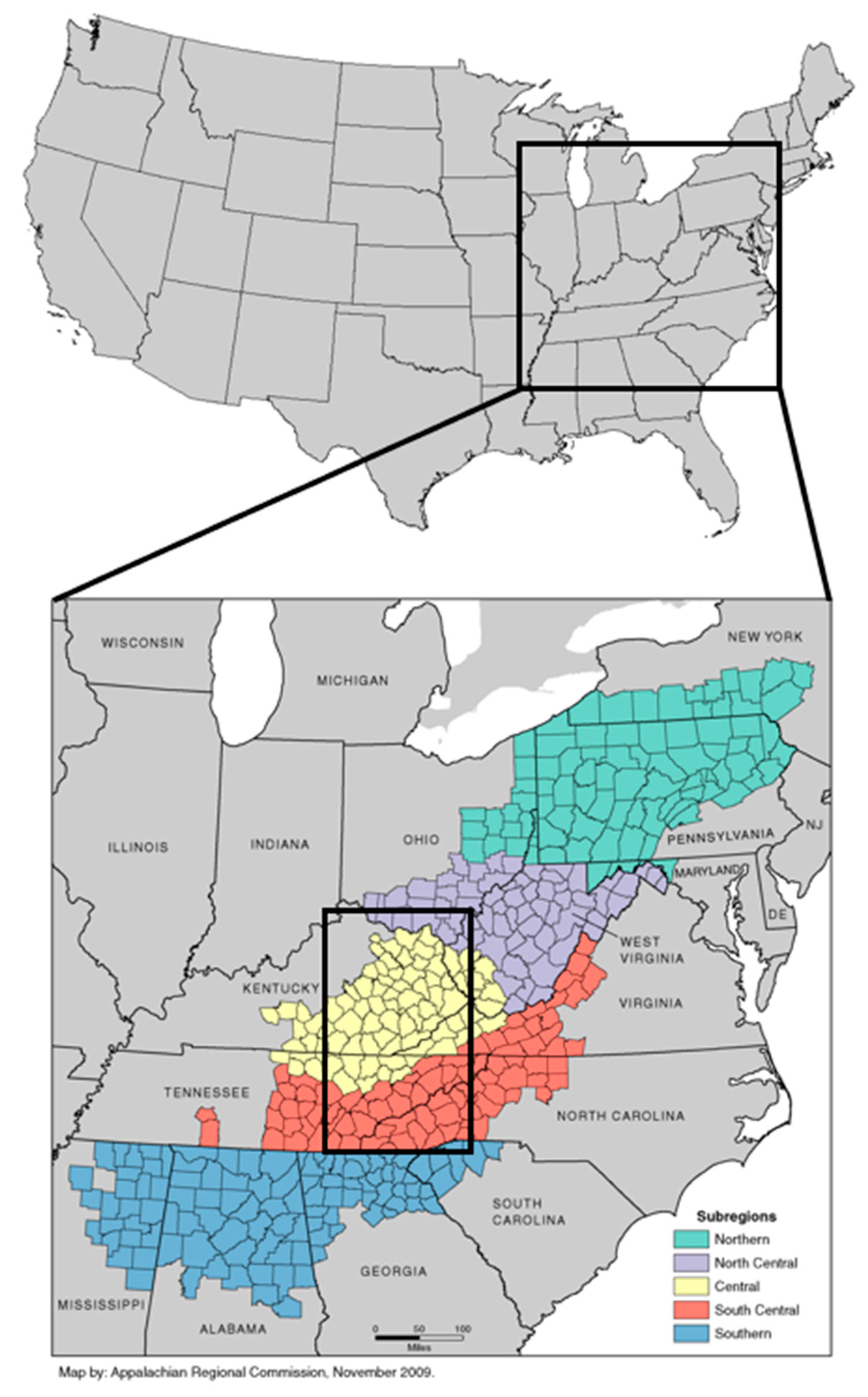
Figure 1. Map of the study region (rectangle in lower map) across the south central (red), central (yellow), and north central (purple) subregions of Appalachia, in relation to the other Appalachian subregions and the contiguous United States. Source: Appalachian Regional Commission [5].
Atmosphere 10 00765 g001
Figure 2. Linear regression trend of the April normalized difference vegetation index (NDVI) per decade (a) and percent of the April NDVI change to the mean NDVI (b) during 1982–2015. Statistically insignificant grid points were masked out at the 10% significance level, and only the grid points with statistically significant vegetation changes re shown here. The dotted rectangle represents the domain for NDVI extraction.
Atmosphere 10 00765 g002
Figure 3. Detrended composite difference analyses of latent heat (a), sensible heat (b) fluxes (W/m2), 2 m-specific humidity at 2 m (g/kg) (c), and soil moisture at 0–200 cm (kg/m2) (d) between the nine years of the highest and lowest average NDVI values for 1982–2015. The statistically significant regions were contoured at the 10% significance level.
Atmosphere 10 00765 g003
Figure 4. Detrended correlation coefficients of the extracted NDVI time series with of latent heat (a), sensible heat (b) fluxes, specific humidity at 2 m (c), and soil moisture at 0–200 cm (d) for 1982–2015. The statistically significant regions were contoured at the 10% significance level.
Atmosphere 10 00765 g004
Figure 5. Annual average (a) and April monthly average (b) of the dryness index (DI) values for 1982–2015. A DI value > 1 indicates water-limited areas, and a DI value < 1 indicates energy limited areas.
Atmosphere 10 00765 g005
Figure 6. The proposed biogeophysical process and plausible associated feedback mechanism of vegetation and precipitation in central Appalachia. Solid and dashed arrows represent the processes based on the results from this study and plausible physical processes, respectively.
Atmosphere 10 00765 g006