Spatial-Temporal Variability of Land Surface Dry Anomalies in Climatic Aspect: Biogeophysical Insight by Meteosat Observations and SVAT Modeling

Abstract

The spatial-temporal variability of drought occurrence over Bulgaria is characterized based on long-term records (2007–2018) of Meteosat information and the SVAT model-derived soil moisture availability index (referred to root zone depth, SMAI). Land surface temperature according to the satellite-derived Land Surface Analysis Satellite Application Facility Land Surface Temperature (LSASAF LST) product and SMAI were used to designate land surface state dry anomalies. The utility of LST for drought assessment is tested by statistical comparative analyses, applying two approaches, site-scale quantitative comparison, and evaluation of spatial-temporal consistency between SMAI and LST variability. Pearson correlation and regression modeling techniques were applied. The main results indicate for a synchronized behavior between SMAI and LST during dry spells, as follows: opposite mean seasonal course (March–October); high to strong negative monthly correlation for different microclimate regimes. Negative linear regressions between the anomalies of SMAI and LST (monthly mean), with a strong correlation in their spatial-temporal variability. Qualitative evaluation of spatial-temporal variability dynamics is analyzed using color maps. Drought-prone areas were identified on the bases of LST maps (monthly mean), and it is illustrated they are more vulnerable to vegetation burning as detected by the Meteosat FRP-PIXEL product. The current study provides an advanced framework for using LST retrievals based on IR satellite observations from the geostationary MSG satellite as an alternative tool to SMAI, whose calculation requires the input of many parameters that are not always available.

1. Introduction

Drought is determined by multiple climate variables on multiple time scales. It can feed back upon the atmosphere via biogeophysical and biogeochemical land-atmosphere interactions, potentially affecting the extremes of temperature, precipitation, and other variables [1,2]. The precise quantification of a drought event is a classic issue and a difficult challenge in geoscience. This signifies the importance of understanding the relationships between water supply and water demand. Regions where soil moisture impacts the atmosphere most are transitional zones between dry and wet climates [3], and are recognized as ‘hotspots’ of land-atmosphere coupling. For the present climate, the southern Europe/Mediterranean area has also been identified as such a region [4]. There is wide scientific consensus that southern Europe, and in particular, the Mediterranean region, can be considered as a climate change hotspot, both in the recent, past, and upcoming future [5,6]. This area has experienced a broad increase in drought frequency and severity [7], especially in summer [8,9,10].

Although all types of drought originate from precipitation deficiency, it is insufficient to monitor solely this parameter to assess severity and resultant impacts [11]. The relationships between meteorological drought indicators and agricultural/silvicultural drought impacts vary across Europe [12]. The efforts of the scientific community are focused on joint international activities that make use of numerical modeling and satellite data in establishing the synchronized Drought Information System in Europe, Africa, and Latin America [13]. As indicators, the following geophysical indices are recommended to be used: soil moisture anomalies, indicators optimized for characterizing vegetation water stress, and satellite observations and products.

Soil moisture, terrestrial vegetation, and atmospheric flows are parts of a complex interacting system, characterized by the presence of many feedback mechanisms between the various components. The strength of the interaction between soil, plants, and atmosphere depends highly on scale, and the incorporation of these relations in a common framework needs an extensive knowledge from different temporal and spatial scales of the land surface-atmosphere interactions [14]. Soil–vegetation–atmosphere feedbacks are particularly important in water-limited ecosystems, where water is the main factor controlling vegetation growth.

Therefore, drought as a specific state of the land surface state refers to the ‘dry’ anomalies of biogeophysical cycling. Soil moisture availability (SMA) to vegetation cover is an important variable for evaluating vegetation transpiration and a key factor in models of ecosystem and carbon cycle processes [15], as well as of energy and water budgets of crop canopies. SMA is a basic parameter in mesoscale atmospheric circulation models [16] and forecasting systems [17,18]. Since it is the main determinant of plant systems development, SMA might also be used in the current work as an information source for ‘warnings’ for environmental constraints. The main limitation of SMA calculation is the lack of ground observations of key variables such as soil moisture or evapotranspiration. Approaches that allow obtaining indirect estimates of such land surface parameters are progressively being introduced. The strengths of remotely sensed data lie in providing temporally and spatially continuous information over vegetated surfaces useful for monitoring surface biophysical variables affecting evapotranspiration (ET) [19]. Over the past 50 years, remote sensing has shifted the field away from the reliance on traditional site-based measurements and enabled observations and estimates of key drought-related variables over larger spatial and temporal scales than was previously possible. Nowadays, using satellite-based remote sensing in combination with in situ data is a promising approach for informing Earth surface modeling [20]. A recent review [21] charts the rise of remote sensing for drought monitoring, examining key milestones and technologies for assessing meteorological, agricultural, and hydrological drought events. Agricultural drought (also referred to as soil moisture drought) represents a deficit in soil moisture available to vegetation driven by a precipitation deficit (meteorological drought) [22]. Remotely sensed agricultural drought monitoring can be via measurement of soil moisture content, usually through microwave radar (active) and radiometers (passive) such as SMOS or SMAP (soil moisture active passive), e.g., [23,24], or through the assessment of vegetation using passive multispectral sensors such as Landsat or, more recently, Sentinel-2/-3, e.g., [25,26]. The former represents a direct measurement of soil moisture, while the latter infers this by assessing vegetation condition or productivity.

Land surface temperature is one of the key parameters in the physics of land–surface processes on regional and global scales, combining the results of all surface-atmosphere interactions and energy fluxes between the atmosphere and the ground. For more complex conditions like vegetated surfaces, the physical temperature of the Earth’s surface can refer to an average effective radiative temperature of the canopy and surface [27,28]. The capabilities of the meteorological geostationary satellites of EUMETSAT provide a set of methods for remote sensing of vegetation water stress. During vegetation stress, the vegetation spectral signatures may be substantially modified. The scientific and societal importance of land surface temperature has been obvious for a long time and it has been observed and investigated quantitatively for years, taking into account the following.

Surface temperature is a basic environmental/meteorological parameter that directly affects human life: it influences the function and variability of ecosystems, including agriculture; exercises control on surface-atmosphere exchange of energy, water, gases and aerosols; and is a primary variable of climatology and an indicator of climate change [29].

Due to the close relationship of surface temperature to soil moisture [30,31], it is an important parameter for monitoring changes in surface conditions: remotely sensed land surface temperature (LST) has been investigated for soil water content [32,33,34], water budget components [35], fire risk [36], and many others.

The remotely sensed estimates of canopy minus air temperature are applied as an indicator of crop/grassland water stress [37,38]. Other studies [39,40] link the temperature difference between LST and air temperature at 2 m height to root zone SMA in order to characterize soil moisture conditions. A statistical model for daily prediction of the maximum air temperature during heat wave episodes has been developed using LST as one of the input parameters [41].

The main objective of this study is to characterize the spatiotemporal variability of dry land surface state anomalies using long-term data records for the region of the Eastern Mediterranean (Bulgaria) and to test the sensitivity of skin temperature retrievals from infrared observations by the Meteosat geostationary satellite as a soil moisture indicator in a climatic context. Considering drought anomalies as a biogeophysical process resulting from the coupling between energy–water cycles on a regional scale, the following aims are specifically focused on:

• Characterizing the spatiotemporal variability of drought occurrence based on long-term data records (2007–2018) of a biophysical index, soil moisture availability index (SMAI, [42]) using the SVAT modeling approach).
• Revealing the score of skin temperature retrieval according to the Land Surface Analysis Satellite Application Facility Land Surface Temperature (LSASAF LST) product as a measure of dry surface state on a regional scale considering its consistency with SMAI based on statistical analyses.
• Identifying the most drought-prone regions over Bulgaria.
• Illustrating the effect of drought on fire activity using satellite information [43,44].

2. Material and Methods

Dry land surface state anomalies are studied using numerical comparative analyses of satellite information from Meteosat and numerical modeling of land-atmosphere interaction. The following drought indicators linked to the coupling between the energy and water cycles (and thus considered as biogeophysical indices) are used.

Soil moisture availability index (SMAI), which is developed on the basis of soil moisture (SM) calculated with the Soil–Vegetation–Atmosphere Transfer (’SVAT_bg’) model [42] of the National Institute of Meteorology and Hydrology (NIMH). SMAI has been produced operationally at NIMH since 2010 as a post-processing of the SVAT_bg model and is used in this study as reference information to identify dry anomalies.

Skin temperature retrieval according to the LSASAF LST product, which is based on IR satellite information from Meteosat Second Generation, to be tested for utility in reflecting dry anomalies on a monthly/annual basis.

2.1. SVAT Model and SMAI

The output of the ‘SVAT_bg’ model developed at NIMH [42] is used for characterizing the land surface state. This is a simple 1D site-scale meteorological model that exploits the concept of one layer of vegetated land surface and two levels of moisture availability in the root zone depth. One of the main ‘SVAT_bg’ model output parameters is soil moisture (SM). For the purposes of the current study, the model is parameterized for a grassland cover with albedo equal to 0.24. Calculations start during the spring at an air temperature transition above a threshold of 5 °C.

2.1.1. The Soil Moisture Availability (SMA) Concept

For assessing land surface moisture state, the soil moisture availability (SMA) concept is adopted to serve as an information source for ‘warnings’ of environmental constraints. Based on the ‘SVAT_bg’ model outputs of SM, a quantitative index soil moisture availability index, SMAI has been developed and operationally calculated at a site scale for the region of each NIMH synoptic station twice per day (0600 UTC and 1800 UTC) for 4 soil layers: 0–5 cm; 0–20 cm; 0–50 cm; 0–100 cm. SMAI is applied as a diagnostic tool in the case of soil overmoistening conditions and flood risk [42], and also works in the case of dry environmental conditions, accounting for drought severity [36,45].

2.1.2. Physical Interpretation of SMAI

Multiple equilibrium states in the soil–vegetation–atmosphere system are characterized by different levels of soil moisture availability. The SMA varies between the permanent wilting point (PWP), which defines the minimum soil moisture that a plant requires to prevent wilting, as well as the field moisture capacity (FMC), which is the maximum moisture content of capillaries in equilibrium with the force of gravity. Between FMC and PWP, there is a level of capillarity tearing moisture (CTM), below which SMA sharply drops as a result of a salutatory alteration in soil moisture mobility. The SMA variability through these three equilibrium states depends on soil physics, degree of moisture access to plants, and available precipitation a day before.

2.2. Drought Identification Using SMAI

Based on the considerations in Section 2.1 the SMAI is designed as a 6-level threshold scheme to account for moistening conditions. SMA is expressed by digital values ranging from 0 to 5, which are correspondingly color-coded,

Table 1. Categories of dry/wet classes by the soil moisture availability index (SMAI) following [42].

Category	SMAI Values	SMAI Color-Coding
Drought	0	Red
Drought risk	1	Orange
Dry	2	Yellow
Optimum	3	Green
Wet	4	Light blue
Overmoistening	5	Dark blue

:

The SMAI is calculated for the region of each synoptic station from the operational NIMH network, indicated by symbol (∙) in Figure 1. Values are visualized accordingly to provide information about the land surface state in each one of the 28 main administrative regions of Bulgaria. The inverse distance weighted (IDW) method, GDAL_grid library, was used to interpolate soil moisture in the mesoregions. This method was chosen due to its simplicity and efficiency as demonstrated in applications that aimed to interpolate soil moisture data [46].

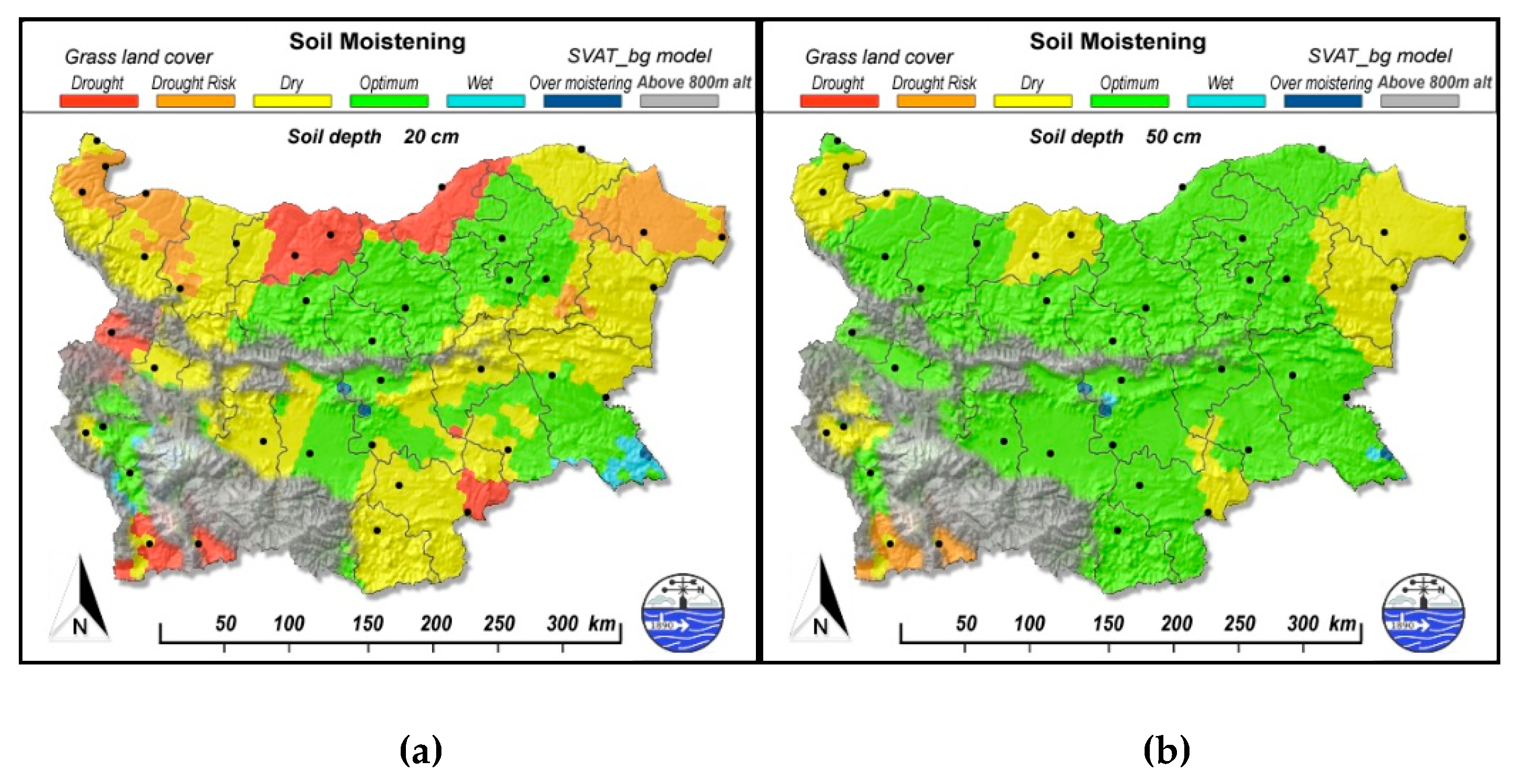
Considering that the soil moisture monitoring observational network in Bulgaria was established to obtain relevant information for use in agricultural productivity modeling, in situ measurements are organized in stations up to 800 m altitude [47]. For that reason, mountain regions are excluded in SMAI maps. In SMAI calculations, the moisture at 50 cm soil depth was used as a reference point, since it is indicative of vegetation activity during persistent dry anomalies.

2.3. The LSASAF LST Product

For the purpose of the current study, skin temperature retrieval according to the LSASAF LST product (MLST, LSA-001) using information from the geostationary Meteosat satellite was applied [48]. The retrieval of LST was based on clear-sky measurements from the MSG system in the thermal infrared window (MSG/SEVIRI channels IR10.8 and IR12.0). Theoretically, LST values can be determined 96 times per day from MSG but, in practice, fewer observations are available due to cloud cover. The identification of cloudy pixels is based on the cloud mask generated by the Nowcasting and Very Short Range Forecasting Satellite Application Facility (NWC SAF) software, https://landsaf.ipma.pt/en/products/land-surface-temperature/lst/. The LST MSG product is computed within the area covered by the MSG disk, every 15 min. The Meteosat LSASAF LST product is received via EUMETCast at the NIMH environment and some missing slots/time intervals are provided by the LSASAF help desk archive for the purposes of this study. The 12-year time series available in HDF5 format are processed by the GDAL_grid translator library and the georeferenced gridded datasets for the region of Bulgaria are visualized, producing maps. Daytime digital LST values at 0900 UTC and 1200 UTC time slots (±30 min to avoid the limitations of cloudy pixels) are inferred at MSG pixel resolution (about 5 km for Bulgaria region) to calculate monthly/annual mean values.

2.4. Numerical Analyses

Based on long-term records (March–October, 2007–2018) of LSASAF LST and the SMAI (referred to root zone depth horizons), a stochastic graphical analysis (boxplots statistics, Pearson correlation coefficient, Pearson′s r, and linear regression techniques) was performed using two approaches—quantitative site-scale comparison, and spatiotemporal variability consistency evaluation. The consistency in the behavior of the two indices was tested in terms of mean seasonal course, spatiotemporal variability on a monthly and annual basis, as well as their anomalous distribution and relations. To perform the comparisons, R language for statistical computing was used [49].

The data for comparative analysis are available at a different spatial resolution from that used in the operational Land Surface Analysis Scheme at NIMH. They are applied for the current study as follows:

SMAI values are calculated on the basis of inputs from meteorological measurements at 36 synoptic stations of the NIMH operational network (for the purposes of this study, only one Synop station is used for each administrative region). Soil moisture can vary significantly with depth and the anomalies at the surface can propagate and influence the dynamics of the entire soil profile [50]. For that reason, SMAI is calculated at 20, 50, and 100 cm, and the mean between 05 and 100 cm soil layers.

LST is derived at MSG pixel resolution and only values in the 1400 grid points of the European Centre for Medium-Range Weather forecasts (ECMWF) global NWP model IFS version O1280 (about 9 km spatial resolution) that cover the region of Bulgaria are used.

At each of these ECMWF grid points, the SMAI values at the nearest synoptic station are considered for calculation and comparison purposes.

Site-scale assessment of mean monthly SMAI at synoptic stations are compared with the averaged LST values from corresponding MSG pixels covering the region of the station using boxplots analyses and Pearson′s r statistics. Color-coded maps for each one of indices (monthly/annual means) and their anomalies (towards 2007–2018) were developed to depict the consistency in spatial-temporal variability between the two indices, including during ‘dry’ and ‘wet’ conditions.

Vulnerability of drought-prone areas to potential fire occurrence over Bulgaria was illustrated using biomass burning detections as shown by the LSASAF Fire Radiative Power-Pixel product for two sample years, 2016 and 2017.

2.5. The LSASAF FRP-PIXEL Product

The FRP-PIXEL product (https://landsaf.ipma.pt/en/products/fire-products/frppixel/) provides information on the location, timing, and fire radiative power (FRP, in Megawatts) output of landscape fires (‘wildfires’) detected every 15 minutes across the full Meteosat disk at the native spatial resolution of the SEVIRI sensor. Measuring FRP and integrating it over the lifetime of a fire provides an estimate of the total fire radiative energy (FRE) released, which for landscape fires should be proportional to the total amount of biomass burned. The pixels containing subpixel-active fire burning at the time of each SEVIRI image area are detected using the so-called geostationary fire thermal anomaly (FTA) algorithm fully described in Wooster et al. and Roberts et al., [43,44]. The product was found to both meet its performance requirements with respect to MODIS, and to be the best performing geostationary fire product currently available at testing. The operational product, disseminated in HDF5 format, was processed by the GDAL_grid library, and confirmed fires were mapped onto a Google Earth image of Bulgaria. Maps with the accumulated fire pixels for the period June–August of 2016 and 2017 were produced.

A summary of all data used for comparative analyses in the current study are presented in

Table 2. Summary of data used and their characteristics.

Data	Temporal Resolution	Spatial Resolution	Type/Source
Soil Moisture Availability Index (SMAI)	Twice daily, 0600 and 1800 UTC	NIMH synoptic station network	SVAT model post-processing/ [36]
Land Surface Temperature (LST)	15 min	SEVIRI, about 5 km over Bulgaria	LSASAF product/ MSG
Fire Radiative Power-Pixel (FRP-Pixel)	15 min	SEVIRI, about 5 km over Bulgaria	FRP-Pixel product/MSG

.

3. Results

3.1. Temporal Variability of Biogeophysical Indices

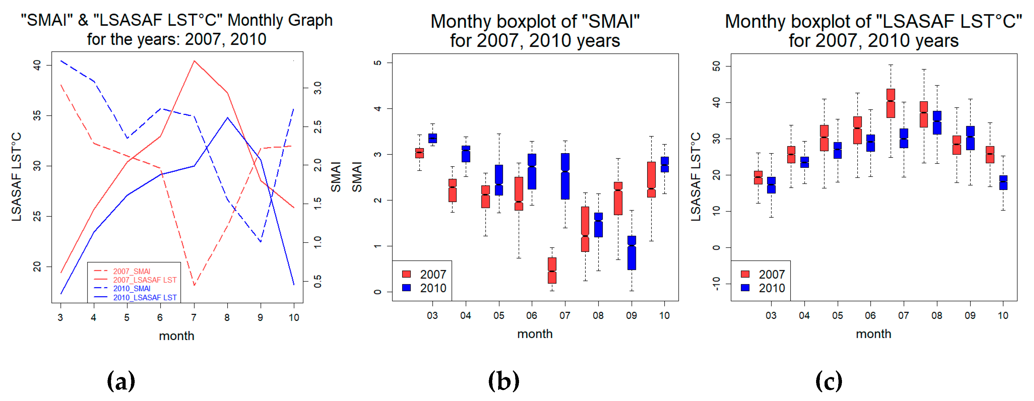
As a first step in the evaluation of the relationships between SMAI and LST, their temporal variability during ‘dry’ and ‘wet’ conditions was compared. The mean seasonal courses (March–October) for two selected ‘dry’/‘wet’ years (2007/2010) within the test period 2007–2018 exhibit similar trends (Figure 2), to summer, LST is increasing. The drought occurrence in July 2007 corresponds to highest mean LST values up to 40 °C while high SMA in July 2010 corresponds to lower LST (around 28 °C). The decreasing SMA is related to increasing of LST for both ‘dry’ and ‘wet’ years/periods, i.e., they have opposite mean annual trends (Figure 2a).

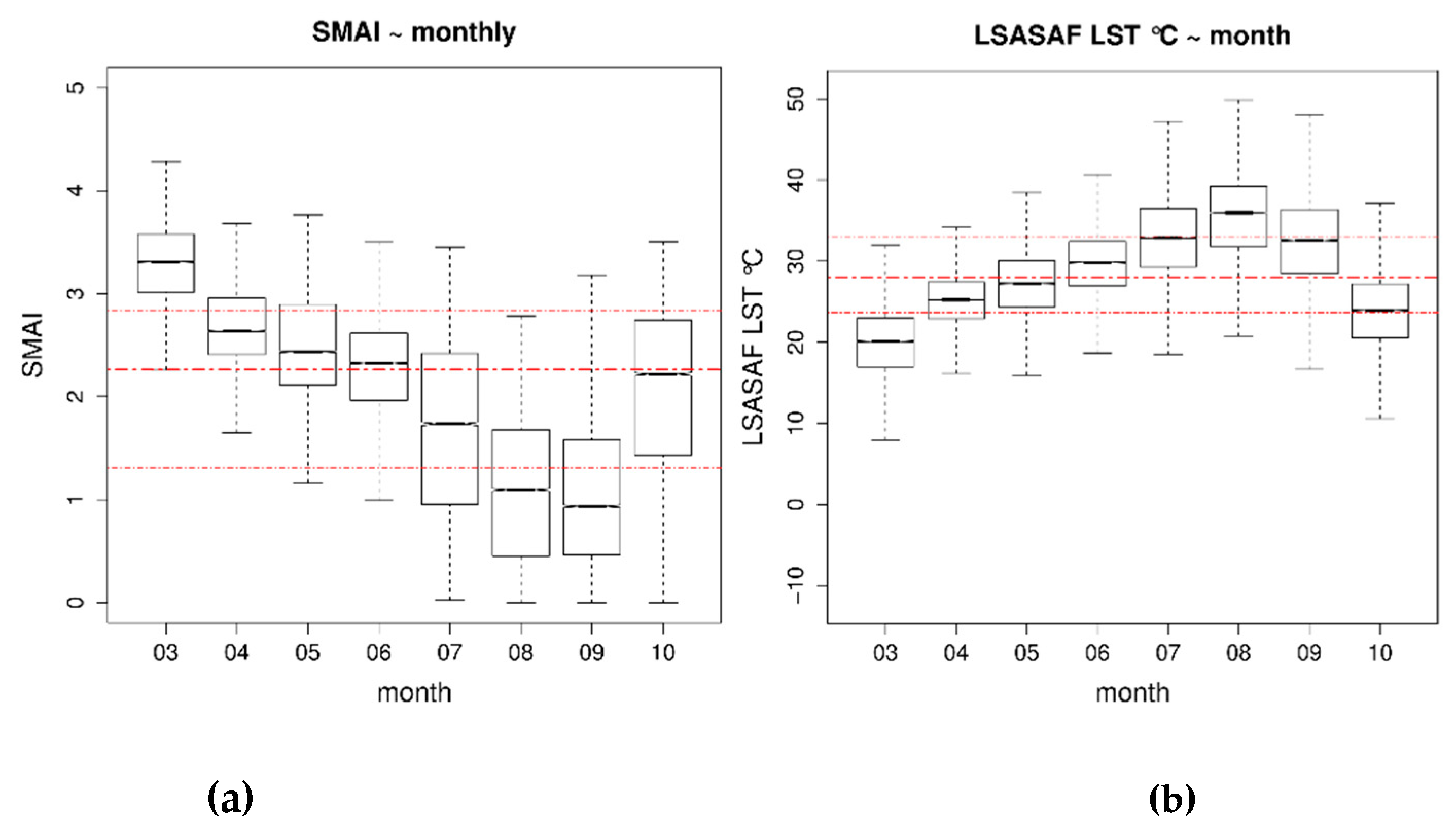
Boxplots of the two indices illustrate their mean values and seasonal variability (Figure 2b,c). The box with notches provides an opportunity for a visual statistical test of a hypothesis for the difference in the medians of the presented data and, thus, to prove the significance of the conclusions drawn below. The attached plots in Figure 2b,c show different aggregation of data by months and years and, thus, by visual comparison of the corresponding notches, it can be found that there is sufficient reason to accept the statistical hypothesis that the medians of all are significantly different.

There is a definite variability of both indices from month to month. During dry periods with depleted SMA, as in July 2007, there is a low variability in SMAI because of the high solar irradiance (leading to high energetic loading) and lack of precipitation. At optimum values of SMAI (March 2007) a low variability is present as well because of small energetic loading, while during wetter periods (July 2010, Aug 2007), the SMAI variation is more significant due to high energetic loading and existing precipitation. LST boxplots from March to October indicate a broader variation during dry periods, in contrast with those during wet periods where the higher SMAI mitigates the land surface heating and, in turn, decreases the amplitude of LST inter-monthly dynamics.

The seasonal course of SMAI and LST for the region of Bulgaria is characterized by their monthly mean values on the basis of the 12-year test period (2007–2018) (Figure 3). The red lines show the median and first and fourth quartile averages of the same statistics for all individual boxplots shown on this plot. They are used to visually assess the degree of difference depending on the month. Based on the boxplot comparative analyses, the following main findings can be drawn.

Mean SMAI and LST have opposed seasonal trends: an initial higher SMAI (optimum moistening) in spring (March) is steadily depleted in parallel to increasing insolation and vegetation development; it becomes significantly depleted in July (between dry and risk of drought stages according to the SMAI scale), reaches a minimum in August/September (risk of drought and drought, correspondingly), and starts to increase in autumn (October) (Figure 3a). Accordingly, LST starts from lowest mean annual values in March and steadily increases with a maximum in August (mean value of about 35 °C) (Figure 3b).

There is a larger variability in both indices for the period July–October. This means that in summer months, there are stronger anomalies in the two characteristics of land surface state. These larger variations are due to the numerous coupled energy–water cycle reveals, i.e., on the one hand, the fully developed vegetation cover decreases the LST by the cooling effect of evapotranspiration while, on the other hand, the steadily depleted available soil moisture restricts the evapotranspiration and this increases LST values. The two mean courses are well synchronized and reveal the average trends during the growing season. The lowest variability for both indices appears in June when precipitation in Bulgaria is maximum and the SMA is accordingly almost optimal.

In October, SMAI variability continues, highly dependent on precipitation, while LST varies within narrow limits. The solar radiation during that part of the year is low and the vegetation is no longer actively growing, thereby restricting evapotranspiration, and both processes prevent large variations in energetic characteristics.

3.2. Spatial Variability in ‘Dry’ and ‘Wet’ Conditions

To depict spatial variability of SMAI and LST, maps of their monthly mean values over Bulgaria are constructed and visualized. Drought severity is assessed according to the SMAI scale using its monthly averaged values for the location of each synoptic station. LST mean monthly values at 0900 UTC ± 30 min for each ECMWF model grid point over Bulgaria are used. Spatial variability of the two biogeophysical parameters are strongly related to the distribution of energy–water cycles across the climate gradient of Bulgaria and, thus, their evolution is performed for a variety of environmental conditions. Based on NIMH long-term data records of precipitation and ‘SVAT_bg’ model outputs, the results are categorized in two types of experimental evolutions for SMAI and LST:

• Years/months with dominant sensible heat fluxes are selected: In this case, a high energetic loading (i.e., high solar irradiance) but limited precipitation lead to depleted SMA and drought occurrence with different levels of severity. Such years/months are classified as ‘dry’ periods.
• Years/months with dominant latent heat fluxes are selected: In this case, even at a high solar irradiance, precipitation is above norms, soil becomes saturated (and even overmoistened), and evapotranspiration is undisturbed. Such years/months are classified as ‘wet’ periods.

3.2.1. SMAI and LST During Dry Conditions

In the ‘dry’ category, two years with different distribution of precipitation deficits from March to August are considered as examples, namely, 2007 and 2012.

Year 2007 is characterized by deficient precipitation from April up to the beginning of August (NIMH Hydrometeorological Bulletin, 2007). In April, the monthly sum is below the norm for the whole country. In May, for eastern Bulgaria precipitation vary from 35% to 65 % of the monthly norm, while in the rest parts of Bulgaria, values are around the norm. In June, for the most part, precipitation is below the monthly norm, 13–73%. In July, precipitation everywhere is below the monthly norm. Precipitation deficit is a marker, but not a sufficient condition, to constitute the existence of terrestrial drought. Based on the ‘SVAT_bg’ model, having inputs from meteorological data at synoptic stations, mean monthly values of soil moisture availability at different depths along the root zone are calculated.

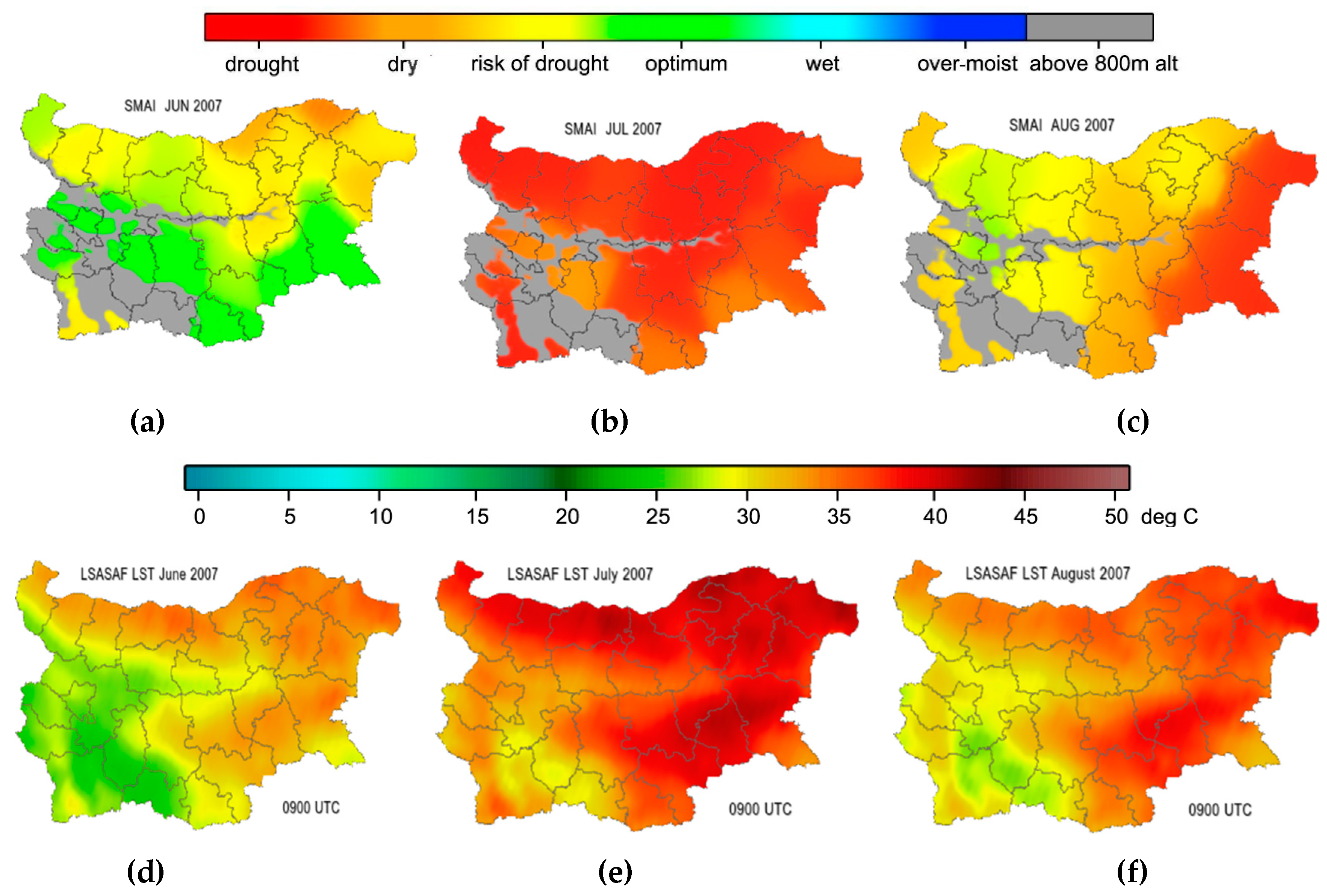
SMAI for 50 cm soil depth (Figure 4a–c) for June, July, August and the corresponding LST spatial distribution for the same period of 2007 (Figure 4d–f) are compared. Visualized maps are used to show the dynamics and variability of moistening and energetic conditions. Maps of SMAI indicate that in June, the northern part of Bulgaria suffers from ‘risk of drought/dry’, which is transformed into severe drought conditions over the whole region in July. In August, precipitation leads to an increase of the SMAI, drought severity declines, but drought remains in the eastern parts where precipitation also stays below the norm for this month. The spatial distribution of LSASAF LST shows a similar pattern: the lower the SMAI (i.e., increased drought severity) the higher the LST. Accumulated terrestrial drought leads to increased land surface temperature, as in July 2007. Qualitative comparison of the color maps reveals a good agreement between the spatial distributions of the two indices: for the regions with low SMAI indicating dry conditions, LST values according to the MSG-based satellite product are high.

Year 2012 is characterized by monthly precipitation below average: in March (4–50% mostly), April (50–120%), June (5–75%), July (0–80%), and August (20–120%). SMAI for 50 cm soil depth is sensitive to reflecting the lack of precipitation and the corresponding deficit in SMA. Spatial distribution for July and August 2012 indicates persistent ‘drought/risk of drought’ for the whole region that is consistent with the distribution of high LST values up to 35–45 °C in the corresponding areas. For 2012, as for 2007, there is a good correspondence in spatial variability of SMAI and LST (not here presented because of similarity with 2007).

3.2.2. SMAI and LST During Wet Conditions

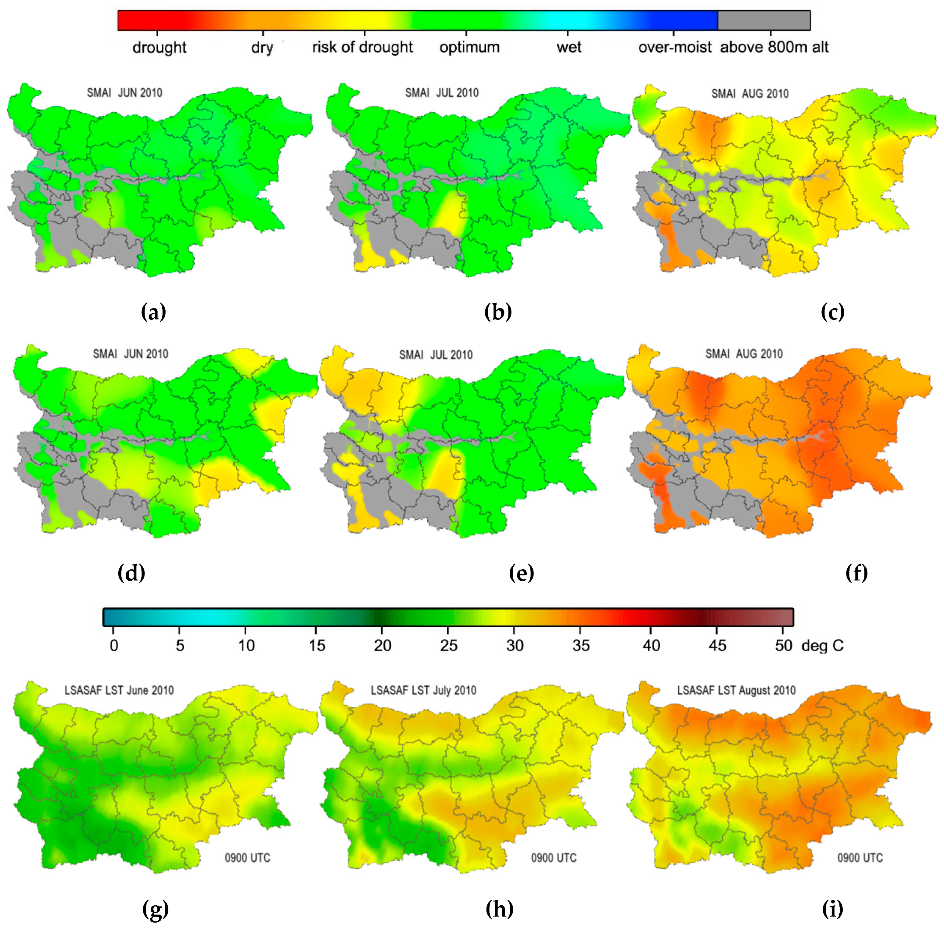
The years 2010 and 2014 are characterized by above-normal precipitation for prolonged periods or for the whole growing season. Year 2010 is characterized by precipitation equal to or above the monthly norms for March, April (small exceptions in eastern parts), May (for most parts of the region), June, July, September (50–150% of norms). The only exception is in August when, in most parts of the country, precipitation is between 0% and 50% of the climatic norms.

Spatial distribution of SMAI for the 50 cm soil layer indicates optimum soil moisture availability from March to July with a slight decrease in August when ‘risk of drought’ is observed over the whole region (Figure 5a–c). SMAI spatial distribution at the 20 cm layer (Figure 5d–f) is also considered because it is more sensitive to evaporative losses of water in wet conditions. For the upper 20 cm soil surface, SMAI indicates ‘risk of drought’ in some regions still in June/July, becoming ‘orange/dry’ for the whole region in August. The distribution of SMAI at 20 cm soil depths more closely corresponds to the increase of LST as a result of high insolation in June–July, and its increases up to 30–35 °C in some parts during August (Figure 5g–i). While during dry periods, there is a good agreement between the spatial distribution of LST and SMAI for 50 cm soil depth (Figure 4), in wet periods, LST spatial distribution is more closely related to SMAI variability at 20 cm soil depth, and LST is lower as shown in Figure 5.

For all months (March–October) of 2014 and for almost all parts of Bulgaria precipitation is above climatic monthly norms (NIMH Hydrometeorological Bulletin, 2014), sometimes 3–3.5 times the norm in July and August that leads to a full soil moisture capacity. The results are consistent with the findings for 2010 (Figure 5), that in ‘wet’ conditions, the LST spatial variability is more closely related to SMAI distribution for 20 cm soil depth than SMA for 50 cm soil depth (because of similarity, maps with the SMAI and LST spatial distribution are not presented here).

3.3. Comparative Analyses of Soil Moisture Anomalies Versus Land Surface Temperature Anomalies

3.3.1. Site-Scale Correlation Analyses

Pearson’s correlation coefficient is used as a measure of the correspondence between SMAI anomalies and LST anomalies. Based on the method of covariance, this test statistic measures the association between the two continuous variables and gives information about the magnitude of the association, or correlation, as well as the direction of the relationship. Pearson’s r of mean monthly anomaly values (regarding the 2007–2018 period) are calculated for the region of each synoptic station from the NIMH operational network.

Table 3. Pearson’s correlation coefficients between the SMAI and LST anomalies for the Nomenclature of Territorial Units for Statistics (NUTS) regions of Bulgaria. NE, northeastern; NC, northcentral; NW, northwest; SE, southeastern; SC, southcentral; SW, southwest.

Station	Soil Layer, cm	March	April	May	Jun	Jul	Aug	Sep	Oct
Dobrich, NE	20	−0.68	−0.59	−0.84	−0.38	−0.78	−0.83	0.09	−0.59
	50	−0.73	−0.38	−0.88	−0.59	−0.78	−0.80	−0.41	−0.40
	100	−0.82	−0.44	−0.61	−0.60	−0.62	−0.77	−0.57	−0.27
Rasgrad, NC	20	−0.36	−0.84	−0.79	−0.64	-.0.62	−0.43	−0.3	−0.46
	50	−0.42	−0.85	−0.73	−0.74	−0.74	−0.83	−0.22	−0.05
	100	−0.41	−0.85	−0.69	−0.67	−0.63	−0.74	−0.59	0.09
Kneza, NW	20	−0.72	−0.76	−0.76	−0.12	−0.85	−0.54	−0.65	−0.51
	50	−0.59	−0.39	−0.81	−0.21	−0.93	−0.82	−0.73	−0.44
	100	−0.7	−0.38	−0.91	0.03	−0.83	−0.94	−0.71	−0.18
Karnobat, SE	20	−0.58	−0.61	−0.61	−0.54	−0.76	−0.74	−0.72	−0.36
	50	−0.67	−0.67	−0.63	−0.56	−0.57	−0.69	−0.66	−0.18
	100	−0.63	−0.68	−0.59	−0.63	−0.6	−0.70	−0.41	0.08
Ivailo, SC	20	−0.73	−0.53	−0.52	−0.42	−0.80	−0.59	−0.70	−0.34
	50	−0.63	−0.63	−0.69	−0.38	−0.80	−0.88	−0.77	−0.40
	100	−0.75	−0.41	−0.70	−0.59	−0.73	−0.88	−0.73	−0.05
Blagoevgrad, SW	20	−0.23	−0.72	−0.65	−0.65	−0.76	−0.53	−0.73	−0.84
	50	−0.09	−0.67	−0.63	−0.43	−0.81	−0.41	−0.79	−0.79
	100	−0.26	−0.62	−0.56	−0.41	−0.81	−0.54	−0.82	−0.57

shows the Pearson correlation between the anomalies of SMAI and LST during the growing season (March–October). Selected stations representative for Nomenclature of Territorial Units for Statistics (NUTS) classification of Bulgaria according to the European Union (https://ec.europa.eu/eurostat/documents/345175/7451602/2016-NUTS-2-map-BG.pdf) are shown. The NUTS classification was set up by Eurostat, the Statistical Office of the European Union, to provide a comprehensive and consistent breakdown of territorial units necessary for collecting, developing and harmonizing regional statistics in the European Union (http://www.europarl.europa.eu/factsheets/en/sheet/99/common-classification-of-territorial-units-or-statistics-nuts-). In this context, Bulgaria is divided into six NUTS—northeastern, NE; northcentral, NC; northwest, NW; southeastern, SE; southcentral, SC; southwest, SW. Calculations are performed for each one of the soil depths, 20, 50, and 100 cm along the root zone. Analyses reveal a common trend in the degree of association between anomalies of SMAI and LST for the NUTS regions.

SMAI and LST appear to be highly negatively correlated during the growing season (Table 3) for all NUTS of Bulgaria. There is a high degree of association between the dry SMAI and warm LST anomalies, exceeding −0.50 most of the time and for most NUTS during the active growing season. The correlation is strong (−0.60 to −0.79) and very strong (above −0.79) in July and August. The strong negative relationship during dry periods highlights the role of LST geostationary retrievals in providing long-term information for drought occurrence and its severity because of the high temporal resolution of MSG. In spring months there is a second peak in correlation between SMAI and LST anomalies (at some stations) but this is not the case of a ‘dry’ land surface anomaly because in this period SMAI indicates optimum moistening and LST is lower (see Figure 2a). In June, when the vegetation cover is fully developed and SMA for that time of year is optimum (precipitation peak for the climate of Bulgaria), the correlation in some regions (NW, SC, SW) becomes weak/very weak due to the cooling effect of non-disturbed evapotranspiration. In October, when the growing season has ended, the relationship between the two indices is low because of the lack of vegetation cover and the periodical precipitation in the autumn. The SW region, Blagoevgrad is an exception to this trend which is related to the longer growing season due to the southern flow of Mediterranean Sea air masses.

SMAI anomalies for all soil depths correlate to a high degree with LST anomalies, and for most of them, the correlation is highest for the 50 cm soil depth. It is demonstrated that in March, the highest correlation is present at 100 cm soil depth. This is due to the very low SMAI anomalies in deep soil layers that correspond to low LST variations in March when the vegetation cover is still at an early stage and insolation is still moderate.

The selected stations in the NC and SW regions, Kneza and Blagoevgrad, respectively, are located in valleys that determine a specific microclimate. A positive relation in Kneza, although very low (r = 0.03), appears in June. For Blagoevgrad, which is in a mountain valley, low correlation in March (respectively low Pearson’s r) is obtained.

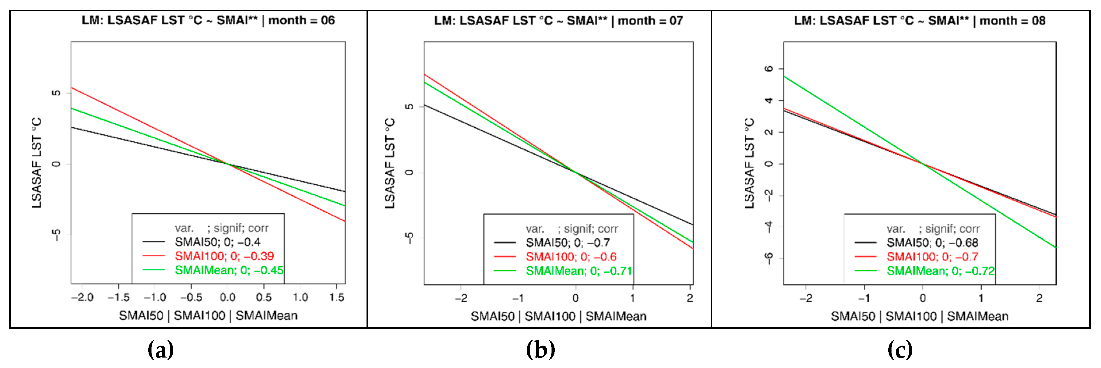
Further evaluation of the relation between SMA anomalies and LST anomalies is performed using the linear regression technique. Mean monthly anomalies from March to October are calculated on the basis of a 12-year period (towards 2007–2018) including the whole region of Bulgaria. SMAI anomalies at different soil layers of 50 and 100 cm were derived. In addition, the mean SMAI for the whole root zone (including 5, 20, 50, and 100 cm soil layers) is considered. Negative linear regression models are estimated to fit the sample distributions for each month with a high level of significance, α = 0.00 (indicated on the graphs, Figure 6).

Using information for the whole region of Bulgaria, the linear regression models confirm the results from site-scale correlation analyses. The correlation of anomalies is minimal in June, still around moderate values, r = −0.45 (Figure 6a). This is the period of full vegetation cover and maximum precipitation for Bulgaria and is related to the high values of SMA and an undisturbed evaporative cooling effect of the land surface. A strong negative relationship between SMAI and LST anomalies is observed in July and August, with correlation coefficients around −0.70 (Figure 6b,c). These are the periods with the most limited rain quantities for the climate of the country, leading to a decrease in the available soil moisture to the vegetation, which restricts evapotranspirative cooling of the vegetated land surface. With strong insolation at the beginning of this period and the following cumulative effects, land surface temperature can increase significantly (above 45 °C).

The values of anomalies of the SMAI and LST indices vary, being in a narrow range during spring and becoming largest for July and August (Figure 6).

It is demonstrated in Figure 6 that a larger correlation, i.e., a stronger relationship between higher warm anomalies of LST and stronger dry anomalies of SMAI occur in the summer months. This result shows that the LSASAF LST product can be used as a tool for drought assessment in the critical period of July–August when most frequently severe dry anomalies occur over southeastern Europe.

3.3.2. Spatial Distribution of Anomalies

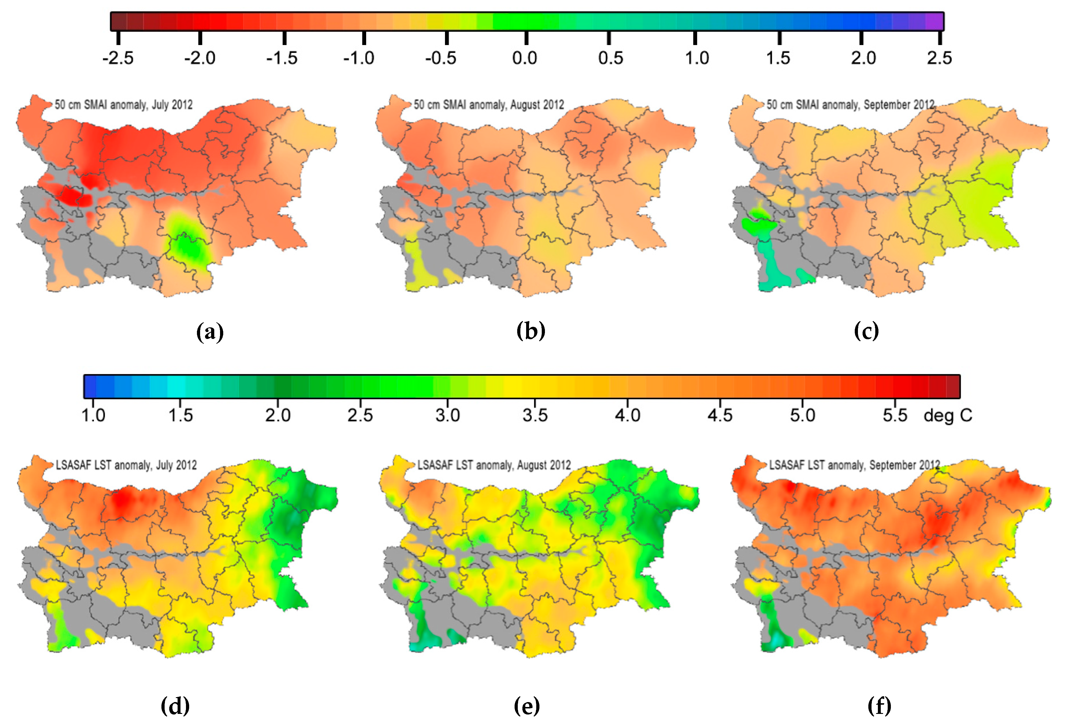
As the next step of the evaluation, the consistency in SMAI and LST behavior and the spatial distribution and variability of their anomalies was analyzed. Mean monthly anomalies were calculated with respect to the entire period of 2007–2018 and visualized in color maps. An example of spatial distribution over Bulgaria of the SMAI and LST anomalies for a selected ‘dry’ period, July–September 2012 is shown on Figure 7. The dry SMAI anomalies and the warm LST anomalies are indicated by reddish colors.

SMAI anomalies at 50 cm soil depth (Figure 7a–c) show that dry soil moisture anomalies are progressively decreasing from July to September. For most parts of Bulgaria, the LST anomalies exhibit a difference from the SMAI trend in 2012: in August (Figure 7e), the LST anomalies slightly decrease compared with July (Figure 7d) and then increase again up to 4–6 °C in September (Figure 7f). The fraction of vegetation cover in September 2012 is relatively lower, leading to a relative decrease in evapotranspiration and, consequently, to an increase in LST and its anomalies.

This behavior of LST anomalies is not observed for the southwestern parts of the country where the LST anomalies decrease progressively from July to September (Figure 7d–f) becoming ‘green’ in September. The southern flow of Mediterranean Sea air masses and the cooling effect of the mountain region mitigate the decrease of the fraction of vegetation cover in the region and the anomalies of the two biogeophysical indices.

However, a very good coincidence in the spatial distributions of ‘dry (in red)’ soil conditions and ‘hot (in red)’ land surface regions is shown, comparing the maps of the spatial distribution anomalies of the biogeophysical indices month by month: locations with the indicated dry negative SMAI anomalies (Figure 7a–c) correspond to regions with positive LST anomalies (Figure 7d–f) for the same period. Some existing mismatches in the degree of SMAI–LST anomalies are due to the highly inhomogeneous land cover as well as the complicated nature of their biogeophysical relations: LST is directly linked to precipitation, cloudiness, solar irradiance, while SMAI is influenced by the cumulative effect of these meteorological parameters and with functional links with vegetation.

3.3.3. Spatial Variability of Correlation between SMAI and LST Anomalies

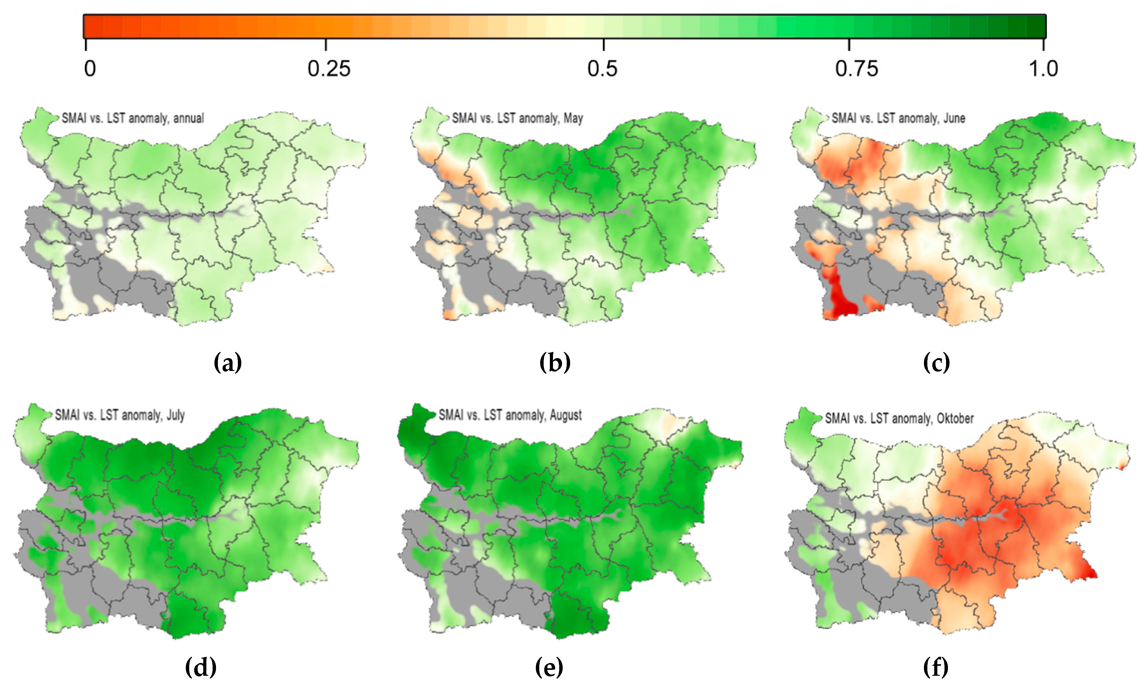
To characterize the spatial variability of LST values to indicate drought over Bulgaria, monthly mean correlations of SMAI and LST anomalies from March to October were calculated for the reference period 2007–2018. Their spatial distribution over Bulgaria is visualized in Figure 8; weak correlation coefficients are in reddish colors, strong correlation coefficients in greenish colors. The following dependences in spatial consistency between SMAI and LSASAF LST anomalies during the different stages of vegetation activity were revealed.

On a mean annual bases (including the whole growing season) the increasing dry anomalies are related to the increase of land surface temperature anomalies. The correlation varies mostly between 0.50 and 0.60 (maximum–0.77) for the whole territory. The color map on Figure 8a indicates that correlations are above moderate, r = −0.45 on mean annual bases.

A strong correlation between the anomalies of the two indices in July and August (coefficients mostly around 0.8, maximum 0.84) was obtained (Figure 8d,e). The behavior of LST closely corresponds to the drought severity as indicated by SMAI for the whole country: the lower the SMAI, the higher the LST. This result is consistent with the findings of past studies [51] that the amplitude of the land surface temperature diurnal cycle was related to soil moisture in regions controlled by thermal inertia, not in transpiration-driven regions [52]. The validation study presented in Ghilain et al. [53] exhibits the same conclusions: results from the comparison show an overall good performance over semiarid regions and degradation toward more wet and vegetated areas. Proceeding from a diurnal cycle [37] to long-term seasonal consideration of correlation between soil moisture and land surface temperature, the results of our study confirm this effect. In the spring and autumn months, the land–atmospheric interaction is a transpiration-driven process that determines the specific seasonal behavior demonstrated in Figure 8b–f.

In May (Figure 8b), the correlation is about 0.60, lower than in July/August for most of the country and even much lower for NUTS in the western mountain part and the mountain region in Southern Bulgaria. During that period of the year soil moisture is high and LST still not so high compared to summer months (see Figure 2a and Figure 3b).

For June (Figure 8c), the correlation tends to become worse. This behavior is due partly to the increased soil moisture as a result of convective precipitation and also to the maximum of solar insolation input, which is related to the increase of LST. The convective activity exhibits its maximum in June and especially near the predominantly mountain areas in the western part of Bulgaria, showing the lowest correlation between SMAI and LST.

In contrast to the behavior in June, the correlation in the western part of Bulgaria is much better in October (Figure 8f), while it is weak over the eastern part of the country. Such a behavior can be explained by the progressive increase of precipitation and soil moisture over eastern Bulgaria due to the enhanced appearance of cyclogenesis over the Aegean Sea that occurs predominantly throughout the cold months (from October to May, [54]). The activation of cyclogenesis in the Eastern Mediterranean basin in October is also confirmed by [55]. The cyclone development often occurs over the Black Sea associated with enhanced latent heat release from warm sea water in October. The increased horizontal moisture flux and resulting increase in moisture flux convergence is consistent with the inland precipitation maximum over the region of eastern Bulgaria in this period [42].

3.3.4. Sensitivity Analyses of Drought-Related Fire Activity

Landscape fires modify the physical and radiative properties of the surface [56,57]. Fires in the Mediterranean are mainly caused by human activities related to agricultural practices. In this regard, identification of the regions most vulnerable to biomass burning is of importance regarding some prevention activities. In general, the process of diagnosing fire risk includes recognition of critical fire weather patterns. Usually, fire weather indices are considered, but this approach is useful for a quick glance across varying time periods and geographic areas to identify possible problems. However, it is important to understand that these criteria could be met in periods where the fuel would not support fire, or conversely, where drought conditions are so profound that an event with less significant weather could still yield a catastrophic fire situation. Therefore, non-meteorological elements can significantly contribute to the enhancement of weather impacting the fire environment such as drought (long term and/or short term), terrain, fuel conditions, and human impacts [37,58,59].

There are many indices reflecting different aspects of drought that are recommended by World Meteorological Organization (WMO) [60]. It is difficult to devise a universal drought index because of the spatial and temporal complexity of drought. Drought indices (standardized precipitation index, Palmer drought index, etc.) are frequently used in a local area and can quickly indicate if the landscape is receptive to fire. The use of these indirect indices results in substantial uncertainties in the resulting analyses. In particular, one of the most widely used, the Palmer drought severity index (PDSI), has been criticized as having several limitations [61,62]. It has been noted that the PDSI may not be comparable between diverse climatological regions, e.g., [63].

An additional layer of analysis uses information on the vegetation (fuel) to indicate the potential for fire activity. The SMAI index (Section 2.2) can provide combined information for both drought and related vegetation stress as a prerequisite of fuel dryness and related fire risk. Remote sensing data are sensitive to the vegetation drought response and enhance capabilities for drought monitoring and detection. 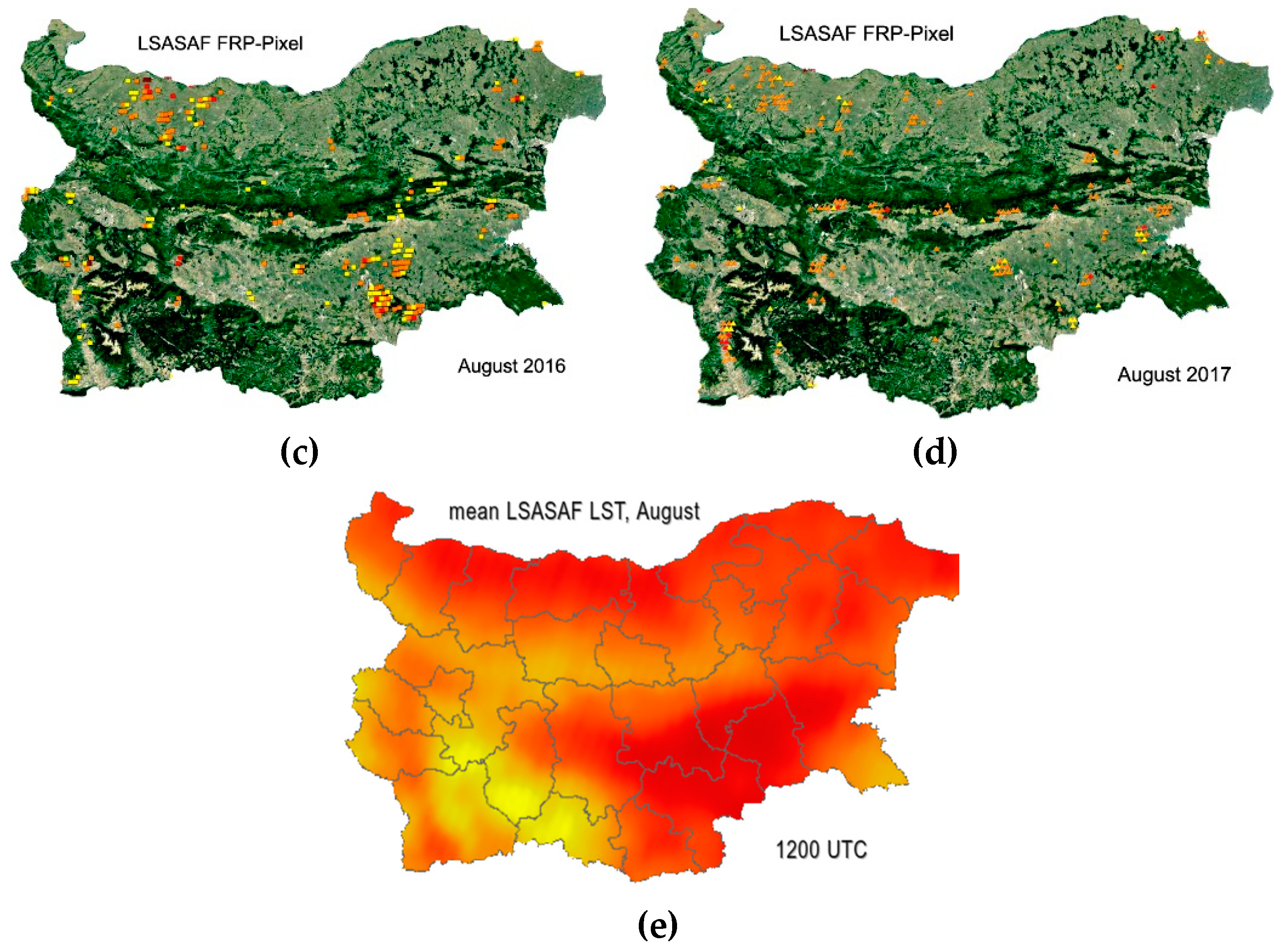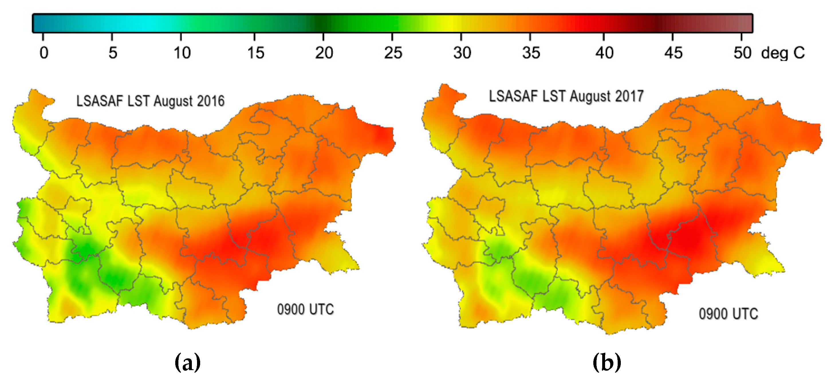The high correlation between SMAI and LST anomalies (Figure 8d,e) reveals that LST derived from operational meteorological satellites can be used as an alternative tool to SMAI for drought and, thus, for fire risk assessment. Monthly means of LSASAF LST for August 2016 and 2017 over Bulgaria are presented in Figure 9a,b, considering that this is typically the period with highest fire activity.

Capturing the spatial and temporal variability of biomass burning can be efficiently performed through observation from geostationary meteorological satellites. The active fire detection by the Meteosat FRP-PIXEL product, providing data with 15-minute repeat cycles for the region of southeastern Europe for the summer periods of 2016 and 2017 over Bulgaria are presented in Figure 9c,d.

Comparing Figure 9a,b with Figure 9c,d reveals that the MSG LST product very well indicates the most sensitive areas for wildfires: a large number of detected fires in the northwestern, southwestern, and southeastern parts of Bulgaria correspond to the areas of highest LST. Figure 9a,b shows that, on average, the land surface state assessed by LST is more receptive to fire in August 2016 than in August 2017. This is reflected by the higher fire activity over Bulgaria in the summer of 2016 than in 2017, as demonstrated in Figure 9c,d.

Figure 9e shows monthly mean LSASAF LST values for August averaged over the period 2007–2018. It is shown that the consistent areas of highest fire activity in 2016 and 2017 are also associated with the regions of long-term conditions of highest LST. The spatial variability of fire activity over Bulgaria demonstrated in Figure 9c,d is primarily related to the long-term land surface state characteristics, and also to favorable mesoscale meteorological factors. The significance of LST as a useful parameter for long-term fire risk assessment originates from it providing combined information for both land surface state (drought, vegetation stress) and meteorological (temperature, humidity) elements, which control the fire risk.

4. Discussion

A major characteristic of drought is the presence of extremely low soil moisture, either due to reduced precipitation and/or increased evapotranspiration [64]. This suggests that soil moisture can provide vital signals about drought conditions and its severity. When studying soil moisture deficit, it is usual to pay attention to the correlation between soil moisture anomaly and the following two frequently used drought indices: the standardized precipitation index (SPI) and the standardized precipitation evapotranspiration index (SPEI) [65]. The World Meteorological Organization [65] suggested that the SPI estimated for time intervals between one and six months can be used for agricultural drought monitoring. Previous studies [66,67] have used the SPI as a benchmark to compare soil moisture anomalies.

In the current study, spatiotemporal variability of drought is analyzed using as reference parameter the soil moisture availability to vegetation, SMAI [42]. This biogeophysical index can account for onset/termination of different levels of drought severity being functionally related to soil moisture deficit, while SPI is a precondition for soil moisture deficit on a correlation principle. The obtained results are indicative of a strong functional negative linear relationship between SMAI and LST during periods of dry land surface anomalies. Using a long-term dataset of 12 years of records from the contemporary climate (2007–2018) over Bulgaria, Eastern Mediterranean region, LST is applied in the context of an Essential Climate Variable (ECV). The correlation varies with the changes of the ratio between evapotranspiration and soil moisture during ‘wet/dry’ periods, and it is also related to the type and state of vegetation cover and local climate. Thus, the current study provides an advanced framework for using LST retrievals based on IR satellite observations from the geostationary MSG satellite as a source of information for studying climatic aspects of dry land surface state anomalies in the context of coupled energy and water cycles. The reported behavior of the biophysical parameter LST underlines the role of land-atmosphere interactions for the establishment of dry land surface anomalies in the Eastern Mediterranean.

The physical basis of this framework is the relationship between surface soil temperature and soil moisture. The variations of surface soil temperature are related to soil thermal properties and meteorological factors such as solar radiation, air temperature, relative humidity, wind, etc. When the soil surface is wet, evaporation is a major factor controlling surface heat loss. As the surface layer dries and the soil water supply cannot meet the evaporative demand, soil temperature is largely influenced by thermal inertia. Thus, the change of surface soil temperature can be an indication of soil water content. Idso et al. [32] found a significant relationship between the diurnal range of surface soil temperature and surface soil water content, and reported that the relationship was a function of soil type. The physical mechanism of this relation includes the following influences: changes in soil moisture affect the albedo and thermal diffusivity of the soil and the Bowen ratio (the ratio of the sensible to latent heat fluxes) in the atmospheric surface boundary layer. As the moist soil surface dries out, more of the incoming solar energy is reflected, and a larger fraction of the absorbed energy is used to heat the air and soil [68]. The heat flow into the soil increases at first, then decreases as the soil becomes very dry [69]. This results in higher land surface temperatures, which also influence the rate of drying and evapotranspiration. Therefore, high LST are both a cause and the product in the case of dry periods.

A good agreement was found between the spatial distributions of the two indices: for the regions with low SMAI, there are high LST values according to the LSASAF satellite product. However, for periods characterized by precipitation equal to or above the monthly norms, there was not good agreement between the LST spatial distribution and SMAI for the 50 cm soil layer (Figure 5). In such ’wet’ periods, LST spatial variability is more closely related to SMAI dynamics in the 20 cm soil layer, but the correspondence is still not satisfactory (Figure 5). This result is consistent with the Prigent et al. (2005) [47] conclusion that in areas where the surface temperature is controlled by evaporation, and not by thermal inertia, the diurnal amplitude extracted from the infrared observations is not well correlated with the soil moisture. In our study, this finding of Prigent et al. (2005) is confirmed on a monthly basis and considering the climatic aspect as well. On the other hand, the reported results indicate that for regional assessment of dry land surface anomalies, more deep root zone layers (about 50 cm) are indicative.

The behavior of LST closely corresponds to the drought severity as indicated by SMAI for the whole country in July and August: the lower the SMAI, the higher the LST. Color-coded maps of spatial distribution of the correlation between the anomalies of SMAI and LSASAF LST indicate a strong relationship for the whole region of Bulgaria (correlation coefficient mostly around 0.8, maximum 0.84, Figure 8d,e). For the rest of the growing season, the correlation (above 0.5) is preserved for regions and months where SMA is negative. This indicates that land surface temperature (LSASAF satellite retrievals) can be used as a dry anomaly indicator on a climatic basis. Taking into account that in July and August, the evapotranspiration is limited for the climate regime of Bulgaria, our results are consistent with the findings of Prigent et al. [44], considering that radiation and soil moisture availability are the main drivers of ET at a regional scale [45]. The validation study presented in Ghilain et al. (2015) [51] exhibits the same conclusions: results from the comparison show an overall good performance over semiarid regions.

The main constraint concerning these satellite applications is that MSG LST data are not available for cloudy pixels. The sensitivity of LST to soil moisture and vegetation cover means it is an important component in numerous applications. However, despite their recognized importance in a large number of applications, accurate measurements of surface skin temperatures over continents are not yet available for the whole globe, for clear and cloudy skies, with a time sampling adequate to resolve the diurnal cycle and to analyze synoptic, seasonal, and interannual variability. A contribution in this direction is the GlobTemperature project of ESA’s Earth Observation Envelope Programme (2013–2017) that provides global-scale satellite LST data for research and operational user communities. The outcome from the project is the delivery of the first LST datasets via a dedicated data portal in harmonized data format [70,71]. The GlobTemperature website remains open. The activity continues under the ESA CCI program (http://cci.esa.int/lst), which is expected to have LST climate data records (CDRs) with the first passive microwave time series.

5. Conclusions

Considering that soil water is central to both biogeophysical and biogeochemical interaction processes within the Earth system, this study is a step forward in revealing the climatic aspects of spatiotemporal variability of land surface dry anomalies using LST retrievals from IR observations by geostationary MSG satellites.

As a consequence, we identify that the relationship between soil moisture and land surface temperature can only be regionally and temporally understood by considering regional and temporal variations of their anomalies, taking into account the main drivers of evapotranspiration and their seasonal changes. The results obtained from the use of satellite LST data as a drought indicator, providing climatic information of drought occurrence and severity, encourages their use in other applications. The results obtained on the use of satellite LST data as a drought indicator providing climatic information of drought occurrence and severity encourages their use in other applications.

As illustrated in this study, the significance of LST as a useful parameter for long-term fire risk assessment comes from its origin in providing combined information for both land surface state (drought, vegetation stress) and meteorological parameters (temperature, humidity), which control the fire risk and indicate potential fire occurrences. Contemporary understanding accounts for drought as a main factor affecting wildfire occurrence and size [36,58,72]. Landscape fires in the Mediterranean region are mostly related to human-caused land-use and land-cover change (LULCC) during their agricultural practices. LULCC can drastically alter hydrological and land surface-atmosphere processes. Knowledge about the identification of drought-prone areas on a regional basis is of importance for the purposes of mitigation activities because fires and biomass burning in the region are not only a natural hazard but can also be a climate change driver. Even better results for fire risk assessment and forecast can be obtained by using as indicator the temperature difference between LST and air temperature at 2 m height (LST-T2m) rather than using LST alone [37,64].

Accurately understanding LST behavior at a regional level helps to evaluate the exchange process in models and, when combined with other physical properties such as vegetation and soil moisture, provides a valuable metric of surface state and processes. Based on the framework developed in this study and our experience on work with LST /(LST-T2) applications, further studies might be focused on using CDR of LST from geostationary and polar orbiting satellite missions for short-term and long-term aspects of drought [37,40] analyses, linking land surface ‘dry’ anomalies and related heat waves [41], for crop yield prediction [47]. Of special interest is the link between the coupled biogeophysical and biogeochemical processes and their associated products, like gross primary productivity (GPP), e.g., in [73], and net primary productivity (NPP) of ecosystems in a drought environment.