Analysis of a Precipitation System that Exists above Freezing Level Using a Multi-Parameter Phased Array Weather Radar

Abstract

An X-band multi-parameter phased array weather radar (MP-PAWR) was developed in 2017. The scan concept of the MP-PAWR is electronic scanning in elevation by combining fan beam transmissions and pencil beam receptions with digital beam-forming techniques and mechanical scanning along the azimuth. The MP-PAWR realized three-dimensional (60 km in radius and 15 km in height) observations without gaps of 30 s. Although the MP-PAWR is supposed to be suitable for observations of rapidly changing convective systems, it can be advantageous for observations of stratiform rainfall because of continuous vertical pointing observations and its ability to apply the Velocity Azimuth Display (VAD) method with a constant radius for a vertical profile of dynamic parameters such as divergence and deformation. In this study, a precipitation system that existed mainly above the freezing level (in this case, it was approximately 5 km in height) observed from 14:00 to 17:00 Japan Standard Time on 6 September 2018 was analyzed using MP-PAWR data. The averaged area of the vertical profile of Z, and the Doppler velocity with fixed elevation showed a stationary structure with time. The average differential reflectivity factor (ZDR) profile with fixed elevation angles showed values that were close to zero and increased with height. Similar characteristics were shown in the average Specific Differential Phase (KDP) profile. Vertical pointing data, especially for Z, ZDR, and Doppler velocity, were utilized when the echo passed over the radar site, and the Doppler velocity showed the acceleration of fall speed below the freezing level. The vertical profile of divergence with a fixed radius was calculated using the VAD method, and the vertical velocity was calculated using the fall speed profile from the vertical pointing data and by assuming the vertical velocity at the cloud base was zero. The results indicate that the updraft region corresponds to higher ZDR and KDP regions.

1. Introduction

In recent years, phased array weather radar technology has been developed [1,2,3,4,5]. The dual-polarization radar is one of several radars that have been developed using phased array weather radar technology [6,7]. The main characteristic of a phased array weather radar is that one-dimensional or two-dimensional electrical scanning can be conducted using a one-dimensional or two-dimensional phased array antenna. Both the precipitation radar (PR) onboard the Tropical Rainfall Measuring Mission (TRMM) satellite and the Dual-frequency Precipitation Radar (DPR) on the core observatory of the Global Precipitation Measurement (GPM) electrically scan ±17 degrees from the nadir and switch the transmission/reception direction using a slotted waveguide array antenna. The X-band phased array weather radar (PAWR), developed in Japan [4,5], introduced a slotted waveguide array antenna similar to the TRMM/PR and the GPM/DPR, and performed electronic scanning in elevation. The PAWR transmits using a fan beam and receives 128-element antenna data, and high-resolution elevational resolution is realized using digital beam-forming techniques. The MP-PAWR ([7]) is a dual-polarization version of the PAWR. By changing the one-dimensional slotted waveguide antenna to a two-dimensional patched antenna, the MP-PAWR realizes electronic elevation scanning with dual-polarization observations. MP-PAWR has been installed at Saitama University (approximately 30 km north of Tokyo) since the end of 2017, and it has been in full operation since March 2018. The main feature of the MP-PAWR is that it can perform dual-polarization observations in a radius of 60 km up to an altitude of 15 km within 30 s by combining the electrical scan in the elevational direction (0–90 degrees) and mechanical scanning in the azimuthal direction (0–360 degrees). Assuming that the typical X-band operational radar with a parabolic antenna scans about 15 elevation angles within 5 min, the MP-PAWR can complete three-dimensional scanning ten times faster while covering 0 to 90-degree elevation angles. Therefore, MP-PAWR is suitable for the observation of rapidly changing hazardous convective systems. The resultant data size in unit time becomes one hundred times larger than the operational radar. Because of the very fast acquisition of three-dimensional observations, the MP-PAWR is thought to be suitable for observing cumulonimbus clouds, which develop very fast and occur at a very high altitude near to the tropopause.

A precipitation cloud observed on 6 September 2018 appeared in a height range from approximately 4 to 10 km, and precipitation was not observed on the ground. This precipitation cloud can be categorized as a virga. The Glossary of Meteorology of the American Meteorological Society (http://glossary.ametsoc.org/wiki/Virga) defines a virga as, “frequently seen trailing from altocumulus and altostratus clouds, but also is discernible below the bases of high-level cumuliform clouds from which precipitation is falling into a dry subcloud layer.” The remote sensing of virgas is often performed using vertical observations by using cloud radar and lidar [8]. Virga-type precipitation systems observed by a spaceborne radar were reported by Wang et al. in 2018 [9], and ground-based radar and range-height indicator (RHI) observations of the anvil portion of the mesoscale convective system (MCS) were reported by Evans et al. in 2011 [10]. There are few continuous observations of three-dimensional structures by polarization radar, and even virga may be extremely hazardous to aviation if colder air is able to descend rapidly. In addition, there are few examples of precipitation observations performed by operational radars, and this is because observations at high elevation angles are typically limited for operation radars. In this paper, we analyzed virga-type precipitation clouds by MP-PAWR to extract dynamic information as well as information regarding the physical characteristics of the clouds using dual-polarization observations.

2. Observation and Analysis Method of MP-PAWR Data

The MP-PAWR is an X-band radar that transmits and receives both horizontal and vertical polarization data simultaneously. By combining fan beam transmissions, where the beam width is ~6 degrees, along with pencil beam receptions, it is possible to complete RHI scans electronically with elevation angles ranging from 0 to 90 degrees in ~0.1 s. The azimuthal observations are accomplished by rotating the antenna. With these observations, we can obtain data up to an altitude of 15 km within a radius of 60 km in 30 s, without any gap. The major observation parameters of the MP-PAWR are the radar reflectivity factor (Z), Doppler velocity, differential reflectivity (ZDR), differential phase shift between horizontal and vertical polarization (φDP), and the correlation coefficient between the horizontal and vertical polarization (ρhv). Takahashi et al. [7] detailed the specifications and performance of the MP-PAWR, and they found that the minimum sensitivity of the radar to be approximately 12 dBZ at a range of 30 km. Regarding the calibration of ZDR, a simple calibration using zenith observations was found to be insufficient. In the MP-PAWR configuration, the antenna pattern of the transmitting fan beam and the receiving pencil beam greatly affected the ZDR estimation. Therefore, the correction value for ZDR was estimated from the ZDR value of the weak echoes sampled from the area, where the attenuation could be ignored for each elevation angle by assuming that the ZDR value of the weak echo was close to zero. The range of correction is about 1 dB. Please note that I am not aware of a better bias correction method than this, even though the ice crystals show larger ZDR for a weak reflectivity factor. In addition, it was found that the calibration bias between the short pulse and the long pulse, especially in the case of the vertical beam in Z, ZDR, and φDP, should be considered. In this study, values from the long pulse were corrected to match the short pulse observations by considering the continuity of the data.

This study presents data obtained from the analysis of a precipitation cloud observed between 14:00 JST (Japan Standard Time = UTC + 9 h; hereafter, the time is express in JST) and 17:00 JST on 6 September 2018. During this event, three-dimensional data were obtained every 30 s. Figure 1 shows an example of a three-dimensional structure of the radar reflectivity factor at 16:00 JST, showing that the radar echo exists mainly at altitudes from 5 to 10 km. In this figure, virga (precipitation echoes streaks extending downward) were seen, in some places, to an altitude of ~2 km. These were recognized as virgas through time-lapse camera observations. Figure 2 shows the plan position indicator (PPI) images of Z, ρhv, Doppler velocity, ZDR, φDP, and specific differential phase (KDP) with an elevation angle of 9 degrees at the same time interval as in Figure 1. The reason why the elevation angle of 9 degrees was selected is that, as can be seen from Figure 1, almost no echo was observed at the low elevation angle PPIs. Since this situation lasted for more than 3 h, it can be assumed that precipitation particles were generated at a high altitude due to the disturbance of the synoptic scale. The maximum radar reflectivity factor at this time was about 25 dBZ, indicating the formation of precipitation particles in this cloud system. The ρhv values were generally smaller than 0.99 and even less than 0.8, where the weak echo dominated. During long-term observations by the MP-PAWR, the ρhv value was smaller than the typical precipitation values of >0.98. The reason for the low ρhv was not identified, but a possible reason could be the low signal-to-noise ratio (SNR) of the weak echo and the smaller correlation due to the combination of the fan beam and pencil beam with digital beam-forming (DBF) techniques. The ZDR field showed almost constant values close to zero between −0.5 and 0.5 dB. The φDP showed a gradual increase with range, and the KDP exhibited positive values of less than 1 degree/km, except for the echo edge.

For dynamic analysis, the velocity azimuth display (VAD) method was used [11]. The VAD method can be applied for PPI data. In this study, however, various elevation angles of PPI data were used in order to estimate the vertical velocity with a fixed radius of the VAD. Since the vertical velocity was calculated from the integration of divergence vertically, from the bottom, by using the mass continuity equation, calculations with a constant radius are more representative of the scale of interest (here, mesoscale phenomena). The MP-PAWR is the most appropriate tool to apply to the VAD method because it can provide seamless elevation angle data. In the VAD method, the Doppler velocity is expressed as:

$$\begin{array}{ll}{V}_r=& V_{z}sin\theta +\frac{1}{2}r\left[\frac{\partial \overline{u}}{\partial x}+\frac{\partial \overline{v}}{\partial x}\right]+\overline{u_0}cos\theta sin\varphi +\overline{v_0}cos\theta cos\varphi \\ & +\frac{1}{2}r\left[\frac{\partial \overline{v}}{\partial x}+\frac{\partial \overline{u}}{\partial y}\right]co{s}^2\theta sin2\varphi -\frac{1}{2}r\left[\frac{\partial \overline{u}}{\partial x}-\frac{\partial \overline{v}}{\partial y}\right]co{s}^2\theta cos2\varphi \end{array}$$

(1)

where θ is an elevation angle, φ is an azimuth angle, and r is a radius. The u₀ and v₀ terms represent the east–west component and the north–south component of the horizontal wind speed, respectively. As shown in (1), the u- and v-components can be expressed in terms of wave number one in the azimuthal domain. In terms of wave number two in the azimuthal domain, these represent deformations (shearing and stretching, respectively). The wave number zero term represents horizontal divergence and vertical motion of the precipitation particles (V_Z). The term V_Z is the sum total of the vertical wind speed and falling speed of the precipitation particles. Since the vertical motion term is the product of sinθ, this term decreases as the elevation angle decreases. Since the target precipitation system did not have intense convection, it can be assumed that the w is nearly uniform in the horizontal direction for each height. The Doppler velocity data at a 90-degree elevation angle was used to obtain V_Z in this equation. Then, the divergence term was estimated from the wave number zero term. The upward motion was calculated by integrating the divergence with the equation of continuity.

Regarding the physical characteristics of the observed cloud, the ZDR and KDP, as well as the Z, with an elevation angle of 10 degrees or less were used to infer the types of precipitation particles. By combining the dynamic information (vertical air motion) from the VAD and other observations with the polarimetric parameter, the formation process of the precipitation particles and their transition was deduced.

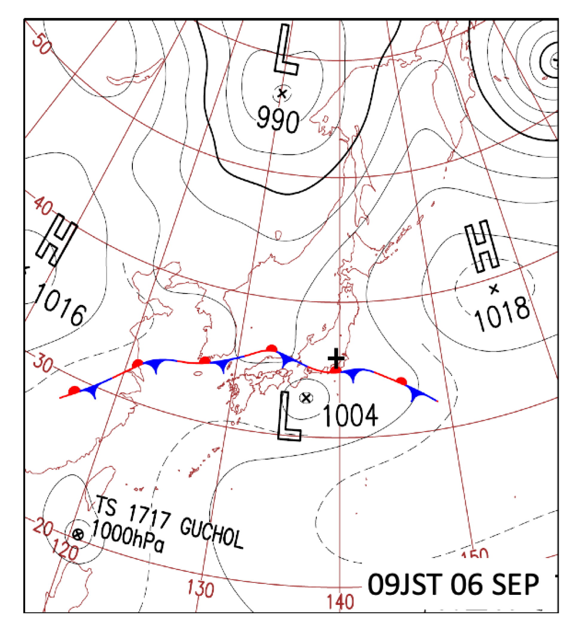
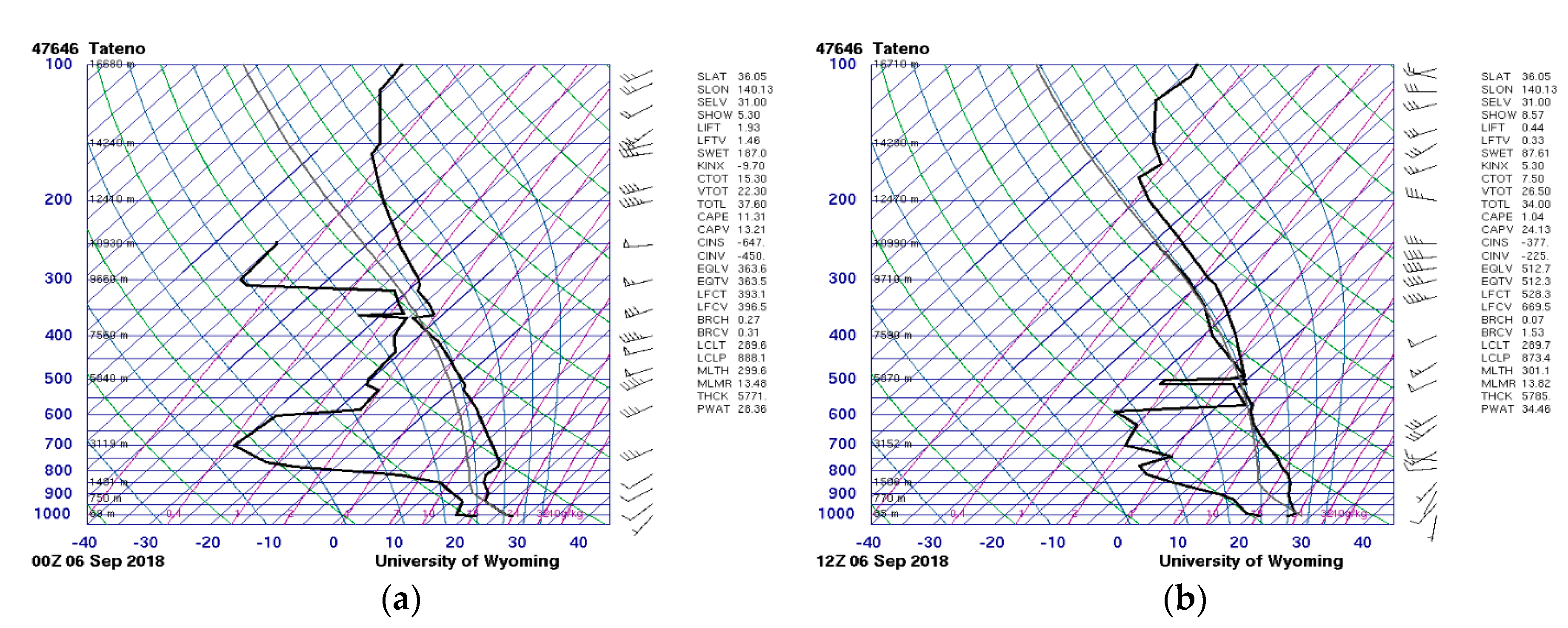
3. Environmental Conditions

Figure 3 shows a weather map from 09:00 JST on 6 September 2018. In this figure, a stagnation front is shown north of a mesoscale, low-pressure system located to the south of the Islands of Japan. The location of the front was just south of the radar site marked with a (+) sign on the chart. Note that these environmental conditions were generated by a typhoon that passed through the area two days prior. The typhoon became an extratropical cyclone at that time (northeast edge, Figure 3). The sounding data from 09:00 JST and 21:00 JST at Tateno (approximately 50 km east–northeast from the radar site) is shown in Figure 4, illustrating that all layers were dry except for at the altitude ~400 hPa at 09:00 JST (Figure 4a). The upper air became moistened above 600 hPa at 21:00 JST (Figure 4b), and the temperature increased by 3–4 degrees below 800 hPa from 09:00 JST to 21:00 JST. Thus, the moist air in the middle layer and the warm air in the lower layer contributed to the formation of the precipitation. Moreover, the freezing level was about ~5000 m (about 5.0 km at 09:00 JST and 4.9 km at 21:00 JST) throughout the day. The convective available potential energy (CAPE) of 1.04 J/kg, the convective inhibition (CIN) of −377 J/kg, and the lifted condensation level (LCL) of ~1200 m indicated that the convective activity on this day was quite low. Figure 5 shows the brightness temperature of the Himawari-8 IR channel (with a wavelength of 10.4 μm) at 16:00 JST. From this figure, a cloud band with low brightness temperature appeared in the observation range of the MP-PAWR, and the minimum brightness temperature was about 225 K, corresponding to an altitude between 11 km and 12 km from radiosonde data at Tateno. This is an interesting finding because this altitude is 1 to 2 km higher than the maximum height of the radar echo, which will be described later. The cloud band was a mesoscale system with a size of ~500 km long by 40 km wide.

4. MP-PAWR Analysis Results

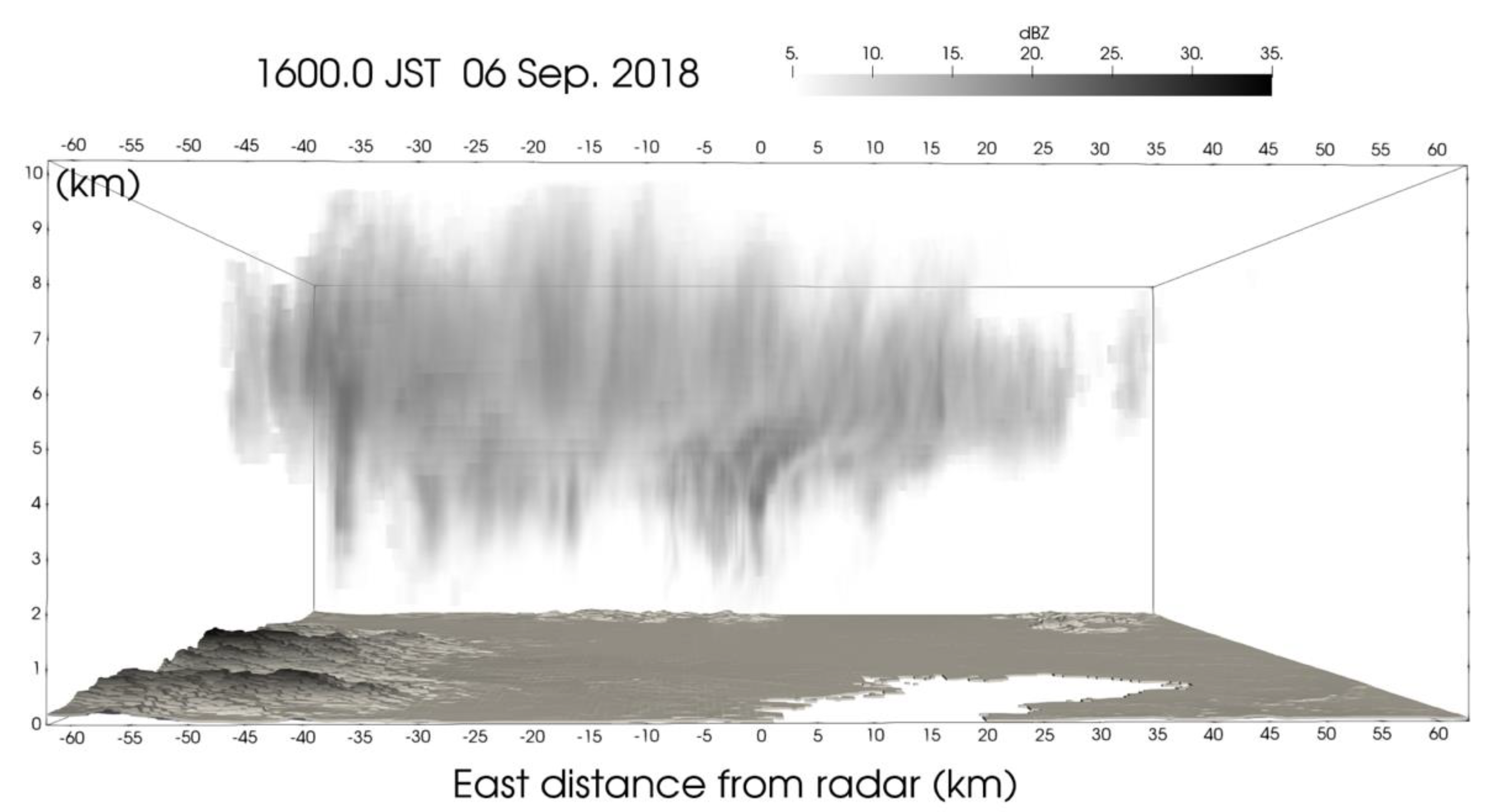
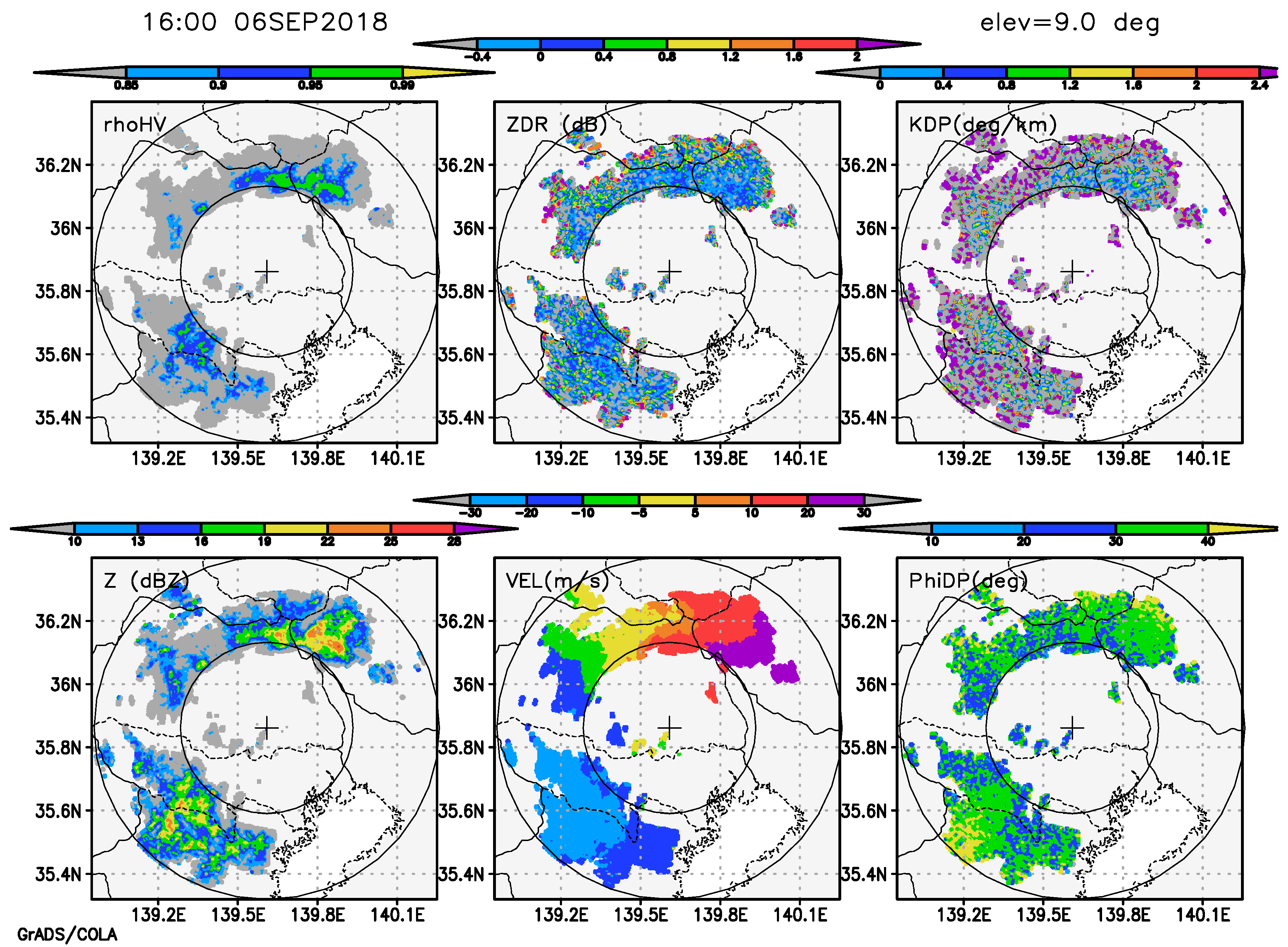
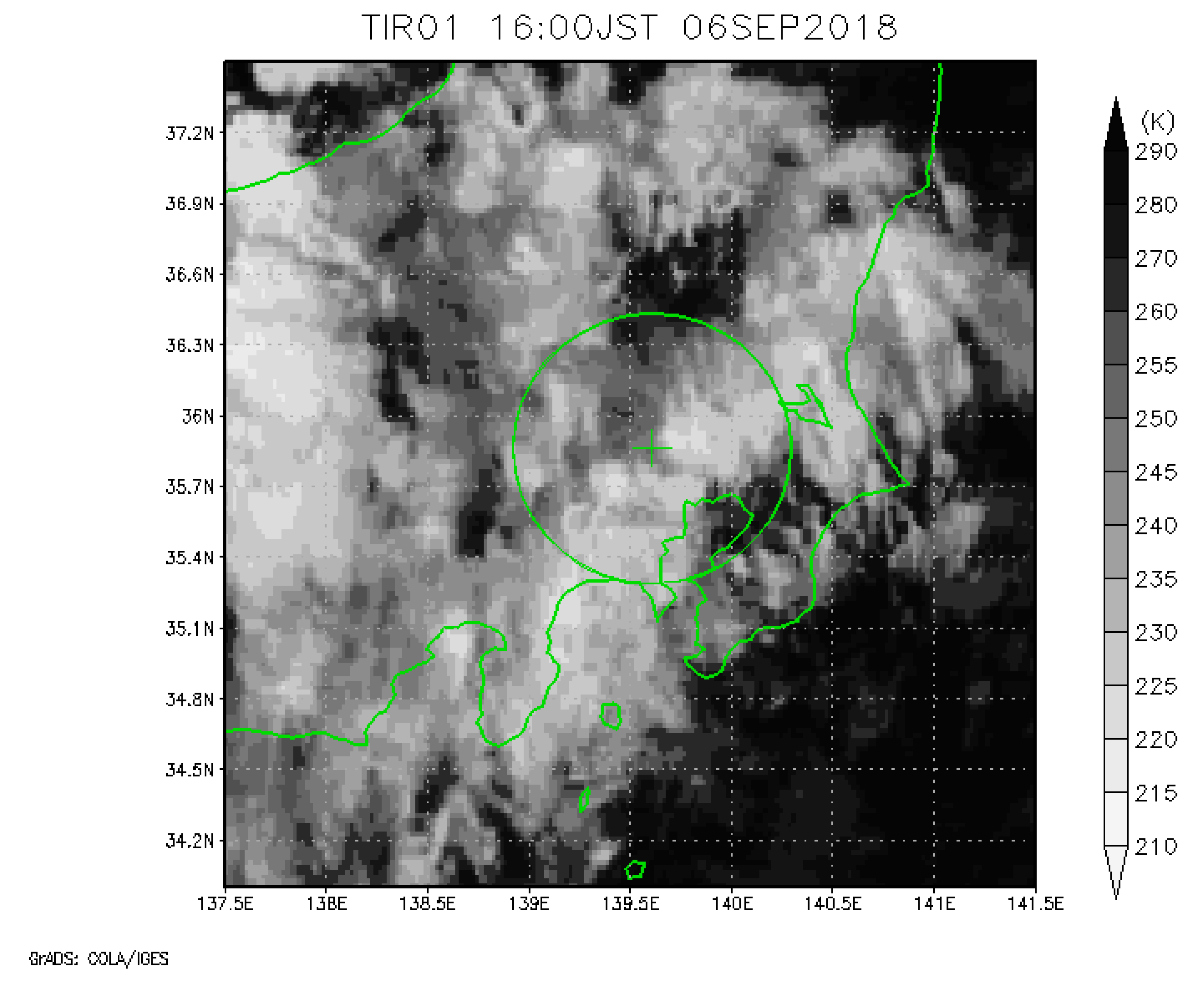
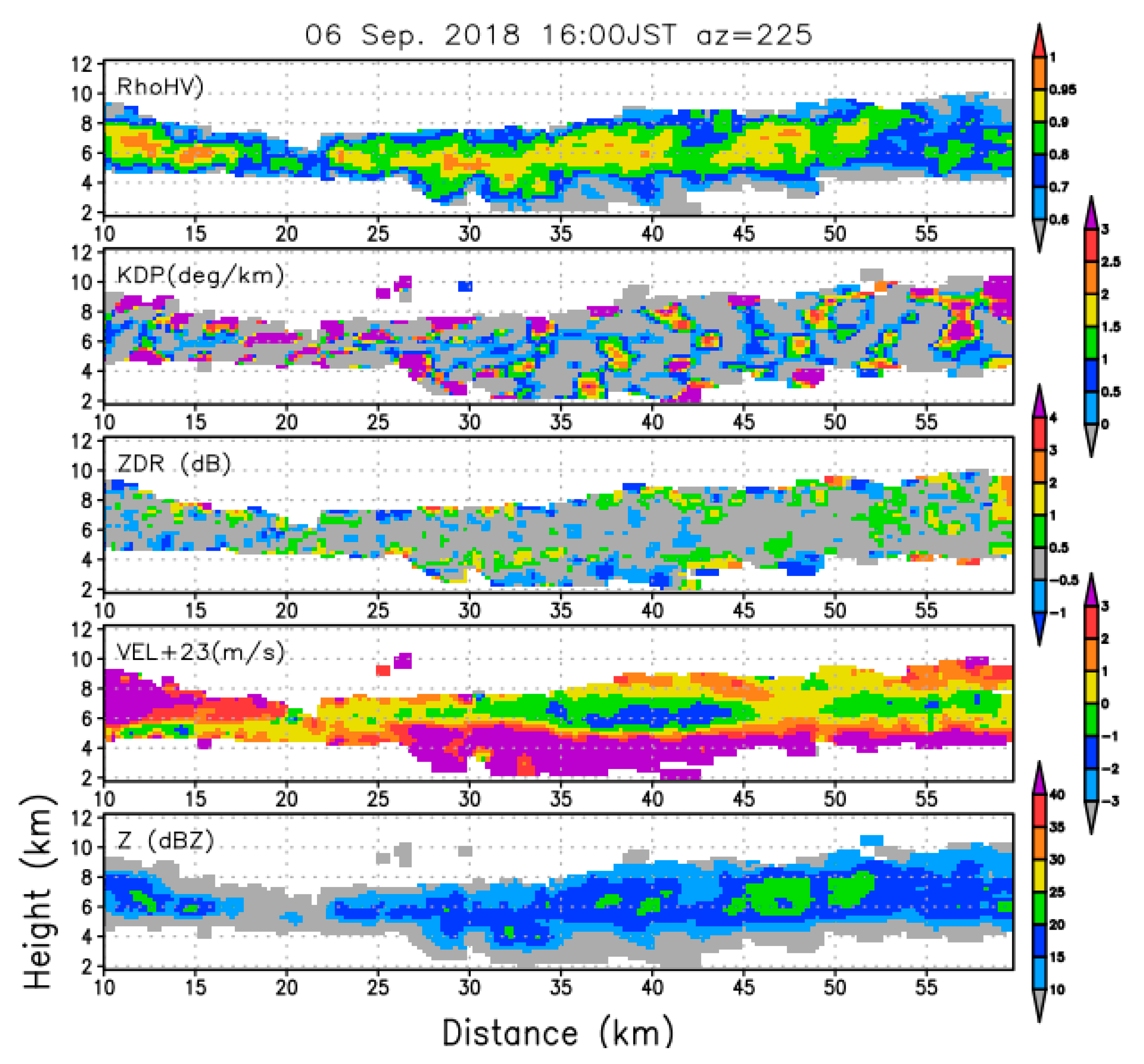
4.1. General Characteristics

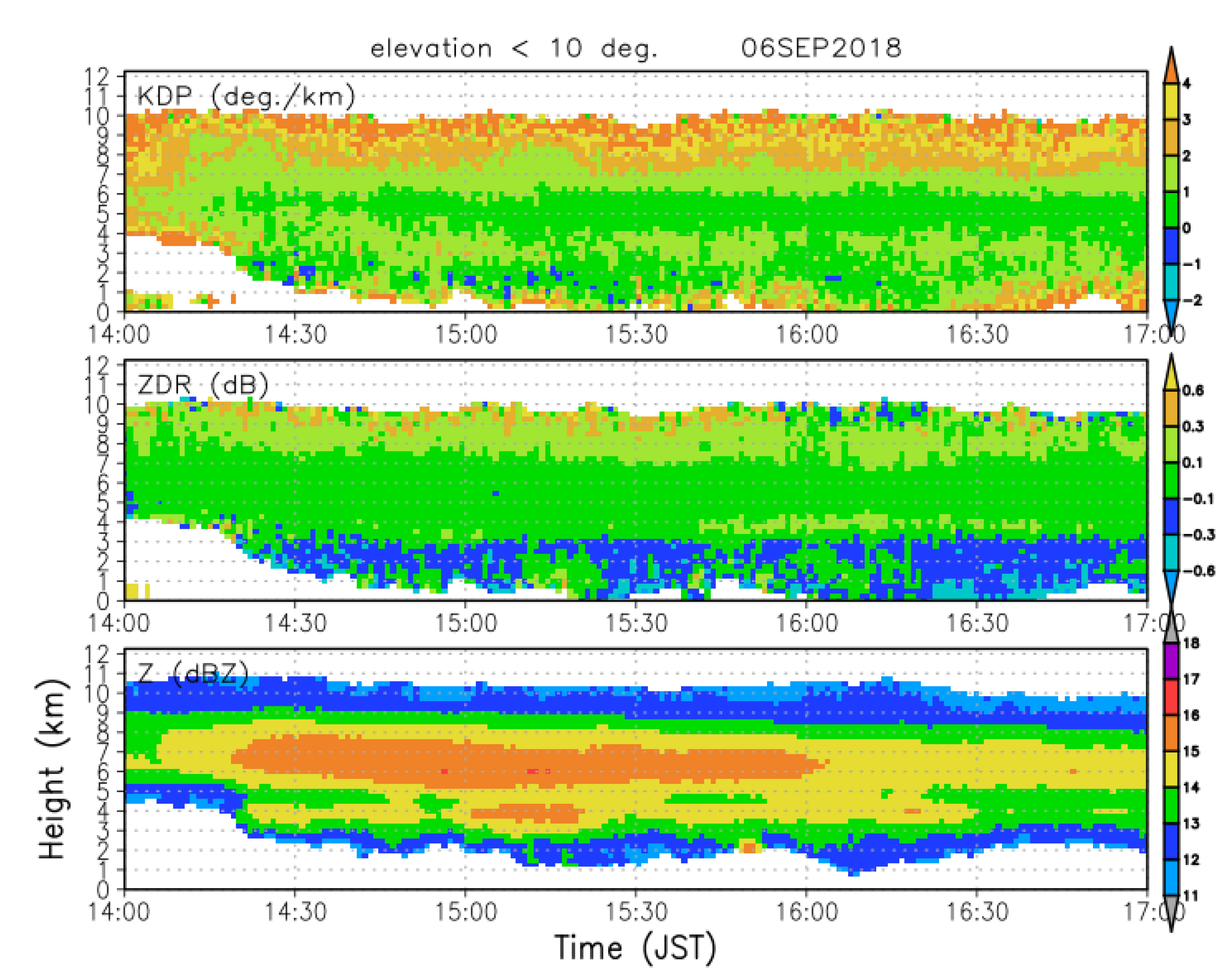
Figure 6 shows the constant altitude plan position indicator (CAPPI) images of Z, Doppler velocity, and ZDR at altitudes of 2 and 5 km from the same time intervals as shown in Figure 1 and Figure 2. The Z at an altitude of 5 km shows a band-like echo running from the southwest to the northeast, in which the echo moved in the northeasterly direction. The overall echo area moved south with time. As shown in Figure 1, only a few small echoes appear at an altitude of 2 km, indicating that almost no precipitation was observed on the ground on this day. The Doppler velocity field at 5 km altitude indicates wind speed corresponding to a general southwesterly wind corresponding to the movement of the echo, suggesting that there was no strong convection in this system. The ZDR was ~0 dB throughout the echo area. The maximum observed radar reflectivity factor was ~25 dBZ, which is considered generally weak, relative to the convective echoes. According to the successive three-dimensional imaging data, Figure 1 clearly captures how a relatively strong echo can occasionally be extended downward. Figure 7 shows a vertical cross section in the upwind direction (225 degrees) at 16:00 JST. Echoes existed mainly in the altitude range from 4 to 8 km, but virga echoes extending below 5 km toward the ground appeared between the distances 25 km and then 45 km, corresponding to the sparse echoes at 2 km altitude from the CAPPI images, as seen in the bottom panels on Figure 6. It should be noted that the freezing level was ~5 km on this day, and the precipitation particles mainly consisted of ice and/or snow except for the virga appearing below the freezing level. Several echo cells were lined up, indicating that the generation of precipitation particles was not uniform. The Doppler velocity field was dominated by the general wind (23 m/s), but fluctuations of up to ± 3 m/s were also seen, indicating the existence of convection. The correspondence between the convergence of the Doppler velocity and the echo cells were seen above 6 km altitude. The ZDR was ~0 dB, except for the echo edge. The ZDR peaks did not correspond with the Z peaks. The KDP profile shows a relatively noisy pattern, but there were places where the maximum KDP above the freezing height corresponded well to the echo, except for the top and bottom edge of the echo, suggesting that there was a mixture of areas where the precipitation particles, like ice crystals, were dominant and other areas where aggregation was dominant. There are several local maxima of KDP near the surface with low Z that may be unreliable because of the low SNR and error relating to the smoothing procedure of φDP before the calculation of KDP. Relatively high ρhv appears above the freezing height. At the area of virga, no clear ρhv dip is seen, suggesting the different structure of stratiform precipitation. These inferences were made based on the study of precipitation particle classification by an X-band polarimetric radar [12].

4.2. Time Series

In order to see the overall characteristics of the system throughout the observation period, spatial averages were taken. Even the echo intensity was not uniformly horizontal, as shown in 4.1. Figure 8 shows the conditional means of observables (Z, ZDR, and KDP) with an elevation angle of <10 degrees that appeared in the observation time range from 14:00 JST to 17:00 JST. Throughout this period, there were no significant changes in the characteristics of the system, and the system appeared to be a relatively steady precipitation system in terms of thickness, the strength of the echo, and the wind field. The Z field (bottom panel, Figure 8) showed a local maxima between 6 and 7 km and then 4 km, and the lower maximum was considered to correspond to the bright band. The ZDR field (middle panel, Figure 8) shows that it was nearly uniform on the horizon, and larger values existed near the top of the echo (~8 km in height). The ZDR value was small and close to zero below the freezing level (5 km in height), but sometimes a larger value was seen near the ground. It was inferred that smaller particles evaporated first during falling, and larger rain drops dominated the echo to increase the ZDR. It should be noted that there still exists a bias of 0.2–0.3 dB in ZDR even though the ZDR value was corrected, as mentioned in Section 3. The KDP field (top panel, Figure 8) shows two local minima around 2 km and then also between 5 and 6 km. The former corresponds to the weak echo near the ground, and the latter corresponds to the height just above the freezing level. The KDP value above 6 km in height increased with height. The reliability of the KDP value near the top edge and the bottom edge of the echo may be low because of the low SNR and the error from the smoothing process of φDP for KDP. The changes in the KDP and the ZDR above the freezing level could be explained by the existence of aggregates just above the freezing level and ice crystals above this layer, greater than 6 km in height. Figure 9 shows a scatter diagram between the Z and KDP and also between the ZDR and KDP above the freezing height. There exists a negative correlation between the Z and KDP, while a positive correlation exists between the ZDR and KDP. One possible explanation for this is that larger ZDR and KDP indicates the existence of ice crystals, and smaller values of ZDR and KDP indicates the existence of aggregated snowflakes. In a scatter plot of Z and KDP, the dispersion of KDP is far below 13 dBZ of the Z, and the reliability of the KDP value is considered to be low due to the influence of noise from the weak echo. In that sense, the KDP value may be valid up to 9 km in height (Figure 8).

Figure 10 shows a time–height cross section of Z, Vr at a 90-degree elevation angle. First, echoes below the freezing level passed over the radar site only around 16:00 JST, corresponding to the precipitation streak (virga) seen in Figure 1. The Doppler velocity below the freezing level was around 5 m/s, which corresponds to the fall velocity of the raindrops. A peak of Z appeared just above the freezing height in Z. The Doppler velocity starts increasing toward the ground below the freezing height. This feature becomes clear by averaging over time, as shown in Figure 11. The Z profile shows a peak at around 6 km in altitude, which may not correspond to the bright band. Around the freezing height, the appearance of a bright band was not clear, and Z gradually decreased toward the ground, indicating the evaporation of precipitation particles. The Doppler velocity profile is a good indicator of the melting process of the precipitation particles: the Doppler velocity of the nadir direction reflects the fall velocity under weak convection. As seen in Figure 10, the profile below the freezing height only reflects the profiles around 16:00 JST. From the top to the freezing height, the doppler velocity increases from 0.5 m/s to 2.5 m/s downward, which corresponds to the fall velocity of ice and snow particles (2.5 m/s is rather fast compared with the typical fall speed of snow, suggesting the downward air motion). At around freezing height, the Doppler velocity gradually increases, starting at an altitude of around 4.5 km. It increased toward the ground, with a peak (<−7 m/s) at 3.5 km in height. The downward velocity decreased below this height. The profiles of Z and Doppler velocity below the freezing level suggest the precipitation particles evaporated, changing the representative size.

4.3. VAD Analysis

Using MP-PAWR observation data, the VAD analyses were conducted at all altitudes with the same radius of calculation. This type of analysis gives more reliable estimations of the mass budget within the column for a given analysis. Since the wave number zero term in Equation (1) consists of the vertical motion term (including updraft/downdraft and fall velocity) and the divergence term, the divergence term itself is estimated using the vertical Doppler velocity, as shown in Figure 11 as the vertical motion term. By using the estimated divergence, the vertical air motion can be calculated via the equation of continuity. The vertical air velocity at the lowest layer of the echo that was taken as zero because of the lower boundary condition. Figure 12 shows examples of the vertical profiles (a—15:51, b—15:56) of wind direction, divergence, vertical wind speed, and the deformation by VAD analysis. In this figure, the VAD was calculated using a radius of 20 km. In both Figure 12a,b, the wind direction and wind speed were almost constant from 5 km (lower limit of calculation) to 7 km. At 15:51 JST, a divergence of 4 × 10⁻⁴/s appeared below 5.5 km, and convergence of about −2 × 10⁻⁴/s existed above 5.5 km. As a result, the downward (negative w) motion was estimated to have a maximum value of approximately −0.3 m/s at ~5.25 km. The profile of the deformation showed the largest value at the bottom, 5 km in height, with a value of 2.5 × 10⁻⁴/s, decreasing with height. At 15:56 JST (Figure 12b), the divergence profile showed a convergence of −1 to −2 × 10⁻⁴/s through the calculated layer, and the upward motion increased with height, where the maximum value of 0.3 m/s occurred near the top of the echo. The profile of the deformation at that time showed a peak at ~5.5 km in height, with a value of about 1.5 × 10⁻⁴/s, and above this height, the value decreased to 1.0 × 10⁻⁴/s. Comparing two panels at 5 min intervals, a sudden change happened within a relatively short time. This may come from the effect of small-scale convection that is not in line with the assumption of the VAD method. In addition, the lower boundary condition of the updraft estimation is unknown. It is discussed in Section 5.2.

Figure 13 shows a time–height cross section of the VAD analysis results. The horizontal wind field shows that more than 22 m/s of wind speed dominated this echo, as shown in Figure 7. A relatively high wind layer, of more than 24 m/s, became dominant through the layer after 14:30 JST, and this high wind region became thinner and shifted downward after 16:00 JST when it became weaker after 16:20 JST. Higher wind speeds appeared at 15:05 JST at an altitude of 7 km and again between 15:45 and 15:55 JST at an altitude below 6 km. The wind direction was generally southwesterly at 6 km in height and changed to the south–southwesterly direction after 15:45 JST. The strong southwesterly wind remained below 6 km. The divergence profiles showed that a divergent field less than 1 × 10⁻⁴/s was dominant below an altitude of 6.5 km before 14:30 JST, and therefore, a downdraft of ~0.2 m/s or less was estimated. Near the top of the echo, the vertical motion changed to an updraft of ~0.2 m/s or less. After 14:40 JST, convergence was dominant in all layers, and its magnitude was −1 × 10⁻⁴/s or more. Sometimes, however, divergence appeared in the lower layer below 6 km. As a result, an updraft of up to 0.4 m/s was estimated near the top of the echo. A particularly strong divergence of more than 1 × 10⁻⁴/s appeared in the lower layer between 15:45 and 15:55 JST, leading the downdraft motion through the layer. This time frame corresponded to the changes in the wind field shown in this figure. A large deformation (1 × 10⁻³/s) was seen between 15:00 and 16:20 JST at an altitude of 6 km, almost matching the strong wind region. In addition, after 16:10 JST, a new, large deformation area appeared at an altitude of 5 km, which corresponded to a low wind area.

5. Discussion

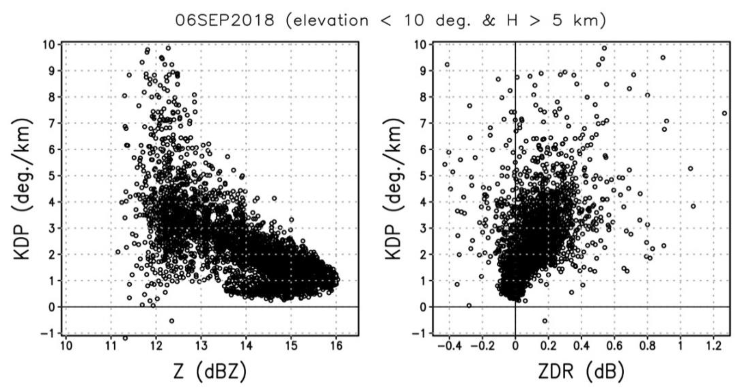
5.1. Precipitation Particle Formation Process

The formation process for precipitation particles was inferred from the characteristics of w (vertical motion, estimated from VAD analysis), Z, ZDR, and KDP. As shown in Figure 12, a characteristic of w is that the updraft appears at an altitude of 6 km or higher, and correspondingly, ZDR and KDP were also increasing upward (Figure 8). From the sounding data, the temperature at 6 km and 7.5 km in height was −8 °C and −15 °C, respectively. The maximum value of Z appeared around 7 km in height (Figure 8). From these, it can be inferred that the ice crystals were formed by the updraft above 6 km in height, and the aggregation progressed in the process of falling to form larger particles, resulting in the larger Z value.

Below the freezing level, virga-type echoes were occasionally observed. As discussed in Figure 11, the Doppler velocity of the vertical pointing data suggested an increase in the downward Doppler velocity above 3.5 km in height, indicating evaporation of the smaller particles with only the larger particle existing at a height of ~3.5 km. Large drops gradually evaporated below 3.5 km in height, and the magnitude of Doppler velocity decreased.

5.2. Estimation of Vertical Air Motion

Since the VAD method assumes the linearity of the wind field and requires appropriate boundary conditions for the calculation of the vertical air motion (w) by using the equation of the mass continuity, the applicability of the VAD method to this case must first be discussed. The target precipitation system in this study was recognized as a relatively uniform system, based on a relatively uniform wind field and a relatively weak echo strength. However, the system did consist of several echo cells, as seen in Figure 7. The lower boundary of the calculation was evaluated at 10 min intervals, which were observed by the L-band wind profiler, or WINDAS, operated by the Kumagaya Regional Meteorological Observatory for the Japan Meteorological Agency, located 38 km north-northwest from the MP-PAWR site [13]. The vertical velocity at 2 km in height showed a downdraft of close to zero, and occasionally, an upward motion was observed. If we assume the lower boundary condition is a downdraft of 1 m/s, then the lower boundary condition cancels out the updraft, which may explain the particle formation. Therefore, it can be concluded that the lower boundary condition was close to zero and potentially less than 1 m/s.

The estimated vertical air motion was less than 0.3 m/s, which is reasonable with the VAD analysis results with different radii. This indicates that the estimated air motion represents mesoscale forcing, meaning the upward/downward motion corresponding to the echo cell may have been larger. In fact, the vertical pointing data indicated that Doppler velocities of near zero and even positive (upward) values existed. In vertical pointing observations, there are fluctuations of about 1 m/s at an altitude of 6 km or higher, so it is not surprising that there was a fluctuation as estimated by the VAD method.

As shown in Figure 12, sometimes sudden changes in the vertical motion appeared. This may be because of the effect of small-scale convection and the uncertainty of lower boundary conditions for the updraft estimation. The former should be investigated further on the error of VAD fitting, and the wind profiler data will help for the latter. A time series of VAD calculation (Figure 13) shows that the vertical structure is rather continuous with some fluctuations, indicating that the general dynamical structure can be deduced with the VAD method.

5.3. Precipitation Formation Mechanism

In this case, precipitation particles formed above 5 km in height, and this precipitation system was not an MCS with an anvil cloud. As can be seen from the weather map, it occurred near a stagnation front at the north end of a cyclone, so it is thought to have been formed as a synoptic scale disturbance. From the reanalysis data (JRA-55 [14]), this system resided in an area located at the north side of the high humidity area at 850 hPa. However, high humidity inflow was seen at 500 hPa, indicating that this layer was the source of the water vapor. The specific humidity above 500 hPa was high on this day since the typhoon passed over the area two days prior. From the WINDAS data, updraft appeared between 2 and 5 km in height after 18:00 JST. The deformation from the VAD analysis suggests that there was a dynamic frontal structure occurring at ~6 km altitude if it is assumed that the high deformation area corresponds to a front. Although a typical virga cloud is considered to appear as either altocumulus or altostratus, the cloud system of this study shows growth to the size of precipitation particles.

6. Conclusions

In this study, three-dimensional analyses of a precipitation system with a thickness of more than 4 km residing above an altitude of 4 km observed from 14:00 to 17:00 JST on 6 September 2018 was investigated using MP-PAWR. The vertical pointing observation data of the MP-PAWR and the VAD analysis, with a constant radius, made it possible to estimate the altitude of the updraft, deformation, as well as dynamic characteristics such as horizontal wind fields. The characteristics of the precipitation particles were estimated from observations of polarimetric parameters, using low elevation angle data below 10 degrees. From these dynamical analyses and analyses of the physical characteristics of the cloud, it was possible to infer the formation process of the precipitation particles.

The observation of the precipitation system analyzed in this study was difficult because of the limited opportunities for collecting data, especially for conventional weather radar because it takes about 5 min to complete three-dimensional observation with limited elevation angles. MP-PAWR has the great advantage of capturing the three-dimensional structure within 30 s without a gap.

In this analysis, the vertical structure of ZDR and KDP are compared with the vertical wind profile obtained by the VAD method. An updraft was observed at a relatively high altitude corresponding to the relatively high KDP and ZDR, suggesting the generation of ice crystals. Below this layer, the peak of Z appears, and it suggests the aggregation of ice crystals. Studies on this type of precipitation system are limited in number but are very important from the viewpoint of radiation balance and global water circulation and aviation operations.

The MP-PAWR is capable of very fast three-dimensional observations by combining a fan beam and a pencil beam. The complete three-dimensional observation, together with the microphysical information and dynamical information, is achieved by this radar. This system has great potential to mitigate the hazardous phenomena, such as severe storms and aviation hazards, as well as the improvement of numerical modeling of precipitation systems.

Issues raised from this study include the calibration of ZDR for each elevation angle because the concept of this radar is to utilize the fan beam transmission, and the calibration between the short pulse range and the long pulse range, especially for 90-degree elevation angles, is an important factor in understanding the system. The former also raises the issue of contamination from the echoes near to the line-of-sight direction; the echo is more intense than the echo of line-of-sight because of the fan beam transmission.

References

1. Zrnic, D.S.; Kimpel, J.F.; Forsyth, D.E.; Shapiro, A.; Crain, G.; Ferek, R.; Heimmer, J.; Benner, W.; McNellis, F.T.; Vogt, R.J. Agile-Beam Phased Array Radar for Weather Observations. Bull. Am. Meteorol. Soc. 2007, 88, 1753–1766. [Google Scholar] [CrossRef]
2. Isom, B.; Palmer, R.; Kelley, R.; Meier, J.; Bodine, D.; Yeary, M.; Cheong, B.L.; Zhang, Y.; Yu, T.Y.; Biggerstaff, M. The Atmospheric Imaging Radar (AIR) for High-Resolution Observations of Severe Weather; IEEE RadarCon (RADAR): Kansas City, MO, USA, 2011; pp. 627–632. [Google Scholar] [CrossRef]
3. Borowska, L.; Zhang, G.; Zrnić, D.S. Considerations for Oversampling in Azimuth on the Phased Array Weather Radar. J. Atmos. Ocean. Technol. 2015, 32, 1614–1629. [Google Scholar] [CrossRef]
4. Yoshikawa, E.; Ushio, T.; Kawasaki, Z.; Yoshida, S.; Morimoto, T.; Mizutani, F.; Wada, M. MMSE Beam Forming on Fast-Scanning Phased Array Weather Radar. IEEE Trans. Geosci. Remote Sens. 2012, 51, 3077–3088. [Google Scholar] [CrossRef]
5. Mizutani, F.; Ushio, T.; Yoshikawa, E.; Shimamura, S.; Kikuchi, H.; Wada, M.; Satoh, S.; Iguchi, T. Fast-Scanning Phased-Array Weather Radar with Angular Imaging Technique. IEEE Trans. Geosci. Remote Sens. 2018, 56, 2664–2673. [Google Scholar] [CrossRef]
6. Heberling, W.; Frasier, S.J. Evaluation of Phased-Array Weather-Radar Polarimetry at X-band. In Proceedings of the 2018 IEEE Radar Conference (RadarConf18), Oklahoma City, OK, USA, 23–27 April 2018; pp. 851–855. [Google Scholar] [CrossRef]
7. Takahashi, N.; Ushio, T.; Nakagawa, K.; Mizutani, F.; Iwanami, K.; Yamaji, A.; Kawagoe, T.; Osada, M.; Ohta, T.; Kawasaki, M. Development of Multi-Parameter Phased Array Weather Radar (MP-PAWR) and Early Detection of Torrential Rainfall and Tornado Risk. J. Disaster Res. 2019, 14, 235–247. [Google Scholar] [CrossRef]
8. Haynes, J.M.; Marchand, R.T.; Luo, Z.; Bodas-Salcedo, A.; Stephens, G.L. A Multipurpose Radar Simulation Package: QuickBeam. Bull. Am. Meteorol. Soc. 2007, 88, 1723–1728. [Google Scholar] [CrossRef]
9. Evans, E.; Stewart, R.E.; Henson, W.; Saunders, K. On Precipitation and Virga over Three Locations during the 1999–2004 Canadian Prairie Drought. Atmosphere-Ocean 2011, 49, 366–379. [Google Scholar] [CrossRef]
10. Wang, Y.; You, Y.; Kulie, M. Global Virga Precipitation Distribution Derived From Three Spaceborne Radars and Its Contribution to the False Radiometer Precipitation Detection. Geophys. Res. Lett. 2018, 45, 4446–4455. [Google Scholar] [CrossRef]
11. Raghavan, S. Radar Meteorology; Artech House: Norwood, MA, USA, 1992. [Google Scholar]
12. Kouketsu, T.; Uyeda, H.; Ohigashi, T.; Oue, M.; Takeuchi, H.; Shinoda, T.; Tsuboki, K.; Kubo, M.; Muramoto, K.I. A hydrometeor classification method for X-band polarimetric radar: Construction and validation focusing on solid hydrometeors under moist environments. J. Atmos. Ocean. Technol. 2015, 32, 2052–2074. [Google Scholar] [CrossRef]
13. Ishihara, M.; Kato, Y.; Abo, T.; Kobayashi, K.; Izumikawa, Y. Characteristics and performance of the operational wind profiler network of the Japan Meteorological Agency. J. Meteor. Soc. Jpn. 2006, 84, 1085–1096. [Google Scholar] [CrossRef]
14. Kobayashi, S.; Ota, Y.; Harada, Y.; Ebita, A.; Moriya, M.; Onoda, H.; Onogi, K.; Kamahori, H.; Kobayashi, C.; Endo, H.; et al. The JRA-55 Reanalysis: General specifications and basic characteristics. J. Meteor. Soc. Jpn. 2015, 93, 5–48. [Google Scholar] [CrossRef] [Green Version]
Figure 1. Three-dimensional view of the virga echo observed on 6 September 2018 by MP-PAWR.
Atmosphere 10 00755 g001
Figure 2. Plan position images (PPI) of the radar reflectivity factor (Z), the correlation coefficient between the horizontal and vertical polarization (ρhv), Doppler velocity, differential reflectivity (ZDR), differential phase shift between horizontal and vertical polarization (φDP) and Specific Differential Phase (KDP) of a 9.0 degree elevation angle 16:00 JST on 6 September 2018. The inner circle indicates the 30 km range, and the outer circle indicates 60 km range from the radar.
Atmosphere 10 00755 g002
Figure 3. Weather chart around Japan at 09:00 JST on 6 September 2018 issued by the Japan Meteorological Agency. The location of MP-PAWR was added to this chart with the plus symbol.
Atmosphere 10 00755 g003
Figure 4. Skew-T diagrams of atmospheric sounding at Tateno at 09:00 JST (a) and 21:00 JST (b) on 6 September 2018. Figures are provided by the University of Wyoming.
Atmosphere 10 00755 g004
Figure 5. IR image of a geostationary meteorological satellite (Himawari-8) at 16:00 JST on 6 September 2018. The plus symbol indicates the location of MP-PAWR, and the circle indicates the observation range (60 km in radius) of MP-PAWR.
Atmosphere 10 00755 g005
Figure 6. CAPPI images of Z, Doppler velocity, and ZDR at 16:00 JST on 6 September 2018. The top three panels show at an altitude of 5 km, and the bottom three panels show at an altitude of 2 km. The inner circle indicates the 30 km range, and the outer circle indicates 60 km range from the radar.
Atmosphere 10 00755 g006
Figure 7. RHI images at the azimuth angle of 225 degrees (upwind direction) at 16:00 JST from MP-PAWR. From the bottom to the top, Z, Doppler velocity relative to the general wind speed (23 m/s), ZDR, KDP, and ρhv.
Atmosphere 10 00755 g007
Figure 8. Time-height cross section of Z, ZDR, and KDP averaged over the scan with the elevation angle of less than 10 degrees.
Atmosphere 10 00755 g008
Figure 9. Scatter plot between Z and KDP (left) and ZDR and KDP (right) from the plot in Figure 8.
Atmosphere 10 00755 g009
Figure 10. Time–height cross section of Z, Doppler velocity of 90-degree elevation angle data.
Atmosphere 10 00755 g010
Figure 11. Vertical profiles of Z, Doppler velocity of time–height cross section in Figure 10 averaged over time.
Atmosphere 10 00755 g011
Figure 12. Examples of the results from Velocity Azimuth Display (VAD) analysis, (a) 15:51 JST and (b) 15:56 JST. From left to right, wind speed (WS), wind direction (WD), divergence (Div.), vertical air motion (w), and deformation (Def.).
Atmosphere 10 00755 g012
Figure 13. Time–height cross section of VAD analysis. From the bottom to the top, wind speed (WS), wind direction (WD), divergence (Div.), vertical air motion (w), and deformation (Def.).
Atmosphere 10 00755 g013