Impacts of Thinning Aircraft Observations on Data Assimilation and Its Prediction during Typhoon Nida (2016)


 and
and
Abstract

1. Introduction
2. Data and Methodology
2.1. Aircraft Observations
2.2. Independent Observations
3. Experiments
3.1. Control Experiment
3.2. Data Assimilation Experiments
3.3. Sensitivity Experiments
4. Results
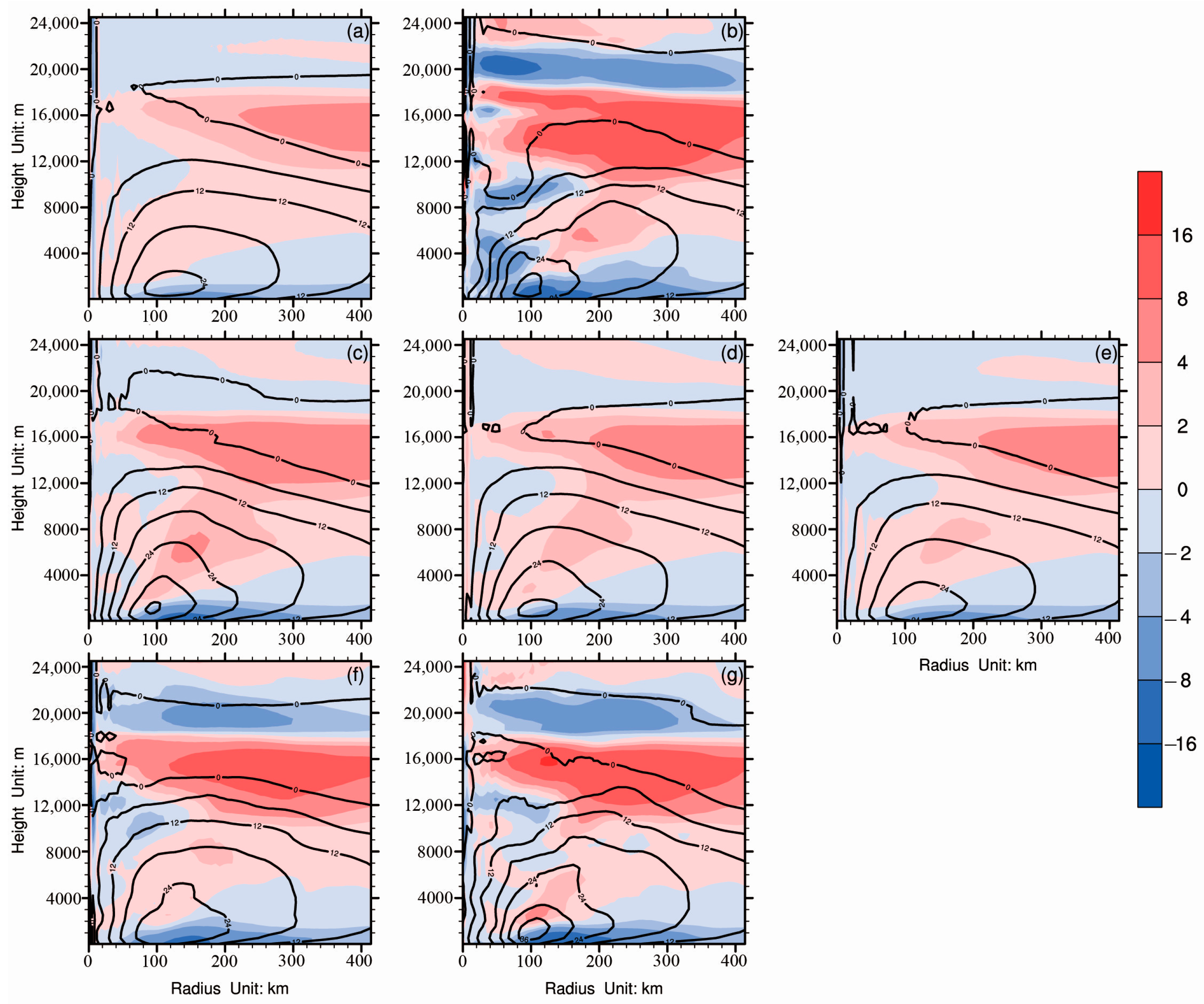
4.1. Typhoon Nida Structures in the Posterior Ensemble Means
4.2. Verifications Against Independent Observations
4.3. Sensitivity Experiments
5. Discussion
6. Conclusions
Author Contributions
Funding
Conflicts of Interest
References
- Landsea, C.W.; Cangialosi, J.P. Have we reached the limits of predictability for tropical cyclone track forecasting? Bull. Am. Meteor. Soc. 2018, 99, 2237–2243. [Google Scholar] [CrossRef]
- Cavallo, S.M.; Torn, R.D.; Snyder, C.; Davis, C.; Wang, W.; Done, J. Evaluation of the Advanced Hurricane WRF Data Assimilation System for the 2009 Atlantic Hurricane Season. Mon. Weather Rev. 2013, 141, 523–541. [Google Scholar] [CrossRef]
- Aberson, S.D.; Black, M.L.; Black, R.A.; Cione, J.J.; Landsea, C.W.; Marks, F.D.; Burpee, R.W. Thirty years of tropical cyclone research with the NOAA P-3 aircraft. Bull. Am. Meteor. Soc. 2006, 87, 1039–1055. [Google Scholar] [CrossRef]
- Wu, C.C.; Chou, K.H.; Lin, P.H.; Aberson, S.D.; Peng, M.S.; Nakazawa, T. The impact of dropwindsonde data on typhoon track forecasts in DOTSTAR. Weather Forecast. 2007, 22, 1157–1176. [Google Scholar] [CrossRef]
- Jung, B.J.; Kim, H.M.; Zhang, F.; Wu, C.C. Effect of targeted dropsonde observations and best track data on the track forecasts of Typhoon Sinlaku (2008) using an Ensemble Kalman Filter. Tellus A 2012, 64, 14984. [Google Scholar] [CrossRef]
- Pu, Z.; Li, X.; Sun, J. Impact of Airborne Doppler Radar Data Assimilation on the Numerical Simulation of Intensity Changes of Hurricane Dennis near a Landfall. J. Atmos. Sci. 2009, 66, 3351–3365. [Google Scholar] [CrossRef]
- Xiao, Q.; Zhang, X.; Davis, C.; Tuttle, J.; Holland, G.; Fitzpatrick, P.J. Experiments of Hurricane Initialization with Airborne Doppler Radar Data for the Advanced Research Hurricane WRF (AHW) Model. Mon. Weather Rev. 2009, 137, 2758–2777. [Google Scholar] [CrossRef]
- Aksoy, A.; Lorsolo, S.; Vukicevic, T.; Sellwood, K.J.; Aberson, S.D.; Zhang, F. The HWRF Hurricane Ensemble Data Assimilation System (HEDAS) for high-resolution data: The impact of airborne Doppler radar observations in an OSSE. Mon. Weather Rev. 2012, 140, 1843–1862. [Google Scholar] [CrossRef]
- Weng, Y.; Zhang, F. Assimilating airborne Doppler radar observations with an ensemble Kalman filter for convection-permitting hurricane initialization and prediction: Katrina (2005). Mon. Weather Rev. 2012, 140, 841–859. [Google Scholar] [CrossRef]
- Zhang, F.; Weng, Y. Predicting Hurricane Intensity and Associated Hazards: A Five-Year Real-Time Forecast Experiment with Assimilation of Airborne Doppler Radar Observations. Bull. Am. Meteor. Soc. 2015, 96, 25–32. [Google Scholar] [CrossRef]
- Aberson, S.D.; Aksoy, A.; Kathryn, J.; Vukicevic, T.; Zhang, X. Assimilation of High-Resolution Tropical Cyclone Observations with an Ensemble Kalman Filter Using HEDAS: Evaluation of 2008–11 HWRF Forecasts. Mon. Weather Rev. 2015, 143, 511–523. [Google Scholar] [CrossRef]
- Chan, P.W.; Hon, K.K.; Foster, S. Wind data collected by a fixed-wing aircraft in the vicinity of a tropical cyclone over the south china coastal waters. Meteorol. Z. 2011, 20, 313–321. [Google Scholar] [CrossRef]
- Sparks, N.; Hon, K.K.; Chan, P.W.; Wang, S.; Chan, J.C.; Lee, T.C.; Toumi, R. Aircraft Observations of Tropical Cyclone Boundary Layer Turbulence over the South China Sea. J. Atmos. Sci. 2019. accepted. [Google Scholar] [CrossRef]
- Gamache, J. Evaluation of a fully-three dimensional variational Doppler analysis technique. In Proceedings of the 28th Conference on Radar Meteorology, Austin, TX, USA, 9–13 September 1997; American Meteorological Society: Boston, MA, USA, 1997; pp. 422–423. [Google Scholar]
- Daley, R. Estimating observation error statistics for atmospheric data assimilation. Ann. Geophys. 1993, 11, 634–647. [Google Scholar]
- Liu, Z.Q.; Rabier, F. The interaction between model resolution, observation resolution and observation density in data assimilation: A one-dimensional study. Q. J. R. Meteorol. Soc. 2002, 128, 1367–1386. [Google Scholar] [CrossRef]
- Liu, Z.Q.; Rabier, F. The potential of high-density observations on Numerical Weather Prediction: A study with simulated observations. Q. J. R. Meteorol. Soc. 2003, 129, 3013–3035. [Google Scholar] [CrossRef]
- Evensen, G. The Ensemble Kalman Filter: Theoretical formulation and practical implementation. Ocean Dyn. 2003, 53, 343–367. [Google Scholar] [CrossRef]
- Zhang, F.; Weng, Y.; Sippel, J.; Meng, Z.; Bishop, C. Cloud-resolving hurricane initialization and prediction through assimilation of Doppler radar observations with an ensemble Kalman filter. Mon. Weather Rev. 2009, 137, 2105–2125. [Google Scholar] [CrossRef]
- Ying, M.; Zhang, W.; Yu, H.; Lu, X.; Feng, J.; Fan, Y.; Zhu, Y.; Chen, D. An Overview of the China Meteorological Administration Tropical Cyclone Database. J. Atmos. Ocean. Technol. 2014, 31, 287–301. [Google Scholar] [CrossRef]
- Knapp, K.R.; Kruk, M.C.; Levinson, D.H.; Diamond, H.J.; Neumann, C.J. The International Best Track Archive for Climate Stewardship (IBTrACS): Unifying tropical cyclone data. Bull. Am. Meteor. Soc. 2010, 91, 363–376. [Google Scholar] [CrossRef]
- Xue, J. Progresses of researches on numerical weather prediction in china: 1999–2002. Adv. Atmos. Sci. 2004, 21, 467–474. [Google Scholar]
- Su, Y.; Shen, X.; Chen, Z.; Zhang, H. A study on the three-dimensional reference atmosphere in GRAPES_GFS: Theoretical design and ideal test. Acta Meteorol. Sin. 2018, 76, 241–254. [Google Scholar]
- Pan, H.L.; Wu, W.S. Implementing a Mass Flux Convective Parameterization Package for the NMC Medium-Range Forecast Model; NMC Office Note 409: Washington, DC, USA, 1995. [Google Scholar]
- Hong, S.Y.; Dudhia, J.; Chen, S.H. A revised approach to ice-microphysical processes for the bulk parameterization of cloud and precipitation. Mon. Weather Rev. 2004, 132, 103–120. [Google Scholar] [CrossRef]
- Hong, S.Y.; Pan, H.L. Nonlocal boundary layer vertical diffusion in a medium-range forecast model. Mon. Weather Rev. 1996, 124, 2322–2339. [Google Scholar] [CrossRef]
- Iacono, M.J.; Delamere, J.S.; Mlawer, E.J.; Shephard, M.W.; Clough, S.A.; Collins, W.D. Radiative forcing by long-lived greenhouse gases: Calculations with the AER radiative transfer models. J. Geophys. Res. 2008, 113, D13103. [Google Scholar] [CrossRef]
- Vukicevic, T.; Aksoy, A.; Reasor, P.; Aberson, S.D.; Sellwood, K.J.; Marks, F. Joint Impact of Forecast Tendency and State Error Biases in Ensemble Kalman Filter Data Assimilation of Inner-Core Tropical Cyclone Observations. Mon. Weather Rev. 2013, 141, 2992–3006. [Google Scholar] [CrossRef]
- Weng, Y.; Zhang, F. Advances in Convection-permitting Tropical Cyclone Analysis and Prediction through EnKF Assimilation of Reconnaissance Aircraft Observations. J. Meteor. Soc. Jpn. 2016, 94, 345–358. [Google Scholar] [CrossRef]
- Evensen, G. Sequential data assimilation with a nonlinear quasi-geostrophic model using Monte Carlo methods to forecast error statistics. J. Geophys. Res. 1994, 99, 10143–10162. [Google Scholar] [CrossRef]
- Houtekamer, P.L.; Zhang, F. Review of the Ensemble Kalman Filter for Atmospheric Data Assimilation. Mon. Weather Rev. 2016, 144, 4490–4530. [Google Scholar] [CrossRef]
- Whitaker, J.S.; Hamill, T.M. Ensemble data assimilation without perturbed observations. Mon. Weather Rev. 2002, 130, 1913–1924. [Google Scholar] [CrossRef]
- Gao, J.; Stensrud, D.J. Assimilation of Reflectivity Data in a Convective-Scale, Cycled 3DVAR Framework with Hydrometeor Classification. J. Atmos. Sci. 2012, 69, 1054–1065. [Google Scholar] [CrossRef]
- Zhang, F.; Snyder, C.; Sun, J. Impacts of Initial Estimate and Observation Availability on Convective-Scale Data Assimilation with an Ensemble Kalman Filter. Mon. Weather Rev. 2004, 132, 1238–1253. [Google Scholar] [CrossRef]
- Gaspari, G.; Cohn, S.E. Construction of correlation functions in two and three dimensions. Q. J. R. Meteorol. Soc. 1999, 125, 723–757. [Google Scholar] [CrossRef]
- Hamrud, M.; Bonavita, M.; Isaksen, L. EnKF and hybrid gain ensemble data assimilation. Part I: EnKF implementation. Mon. Weather Rev. 2015, 143, 4847–4864. [Google Scholar] [CrossRef]
- Chan, J.C.L.; Williams, R.T. Analytical and numerical studies of the beta-effect in tropical cyclone motion. Part I: Zero mean flow. J. Atmos. Sci. 1987, 44, 1257–1265. [Google Scholar] [CrossRef]
- Chan, J.C.L.; Ko, F.M.F.; Lei, Y.M. Relationship between potential vorticity tendency and tropical cyclone motion. J. Atmos. Sci. 2002, 59, 1317–1336. [Google Scholar] [CrossRef]
- Rogers, R.R.; Yau, M.K. A Short Course in Cloud Physics, 3rd ed.; Butterworth-Heinemann: Woburn, MA, USA, 2008; pp. 110–130. [Google Scholar]
- Lu, Y.; Zhang, F. Toward Ensemble Assimilation of Hyperspectral Satellite Observations with Data Compression and Dimension Reduction Using Principal Component Analysis. Mon. Weather Rev. 2019, 147, 3505–3518. [Google Scholar] [CrossRef]
- Aksoy, A. Storm-relative observations in tropical cyclone data assimilation with an ensemble kalman filter. Mon. Weather Rev. 2013, 141, 506–522. [Google Scholar] [CrossRef]


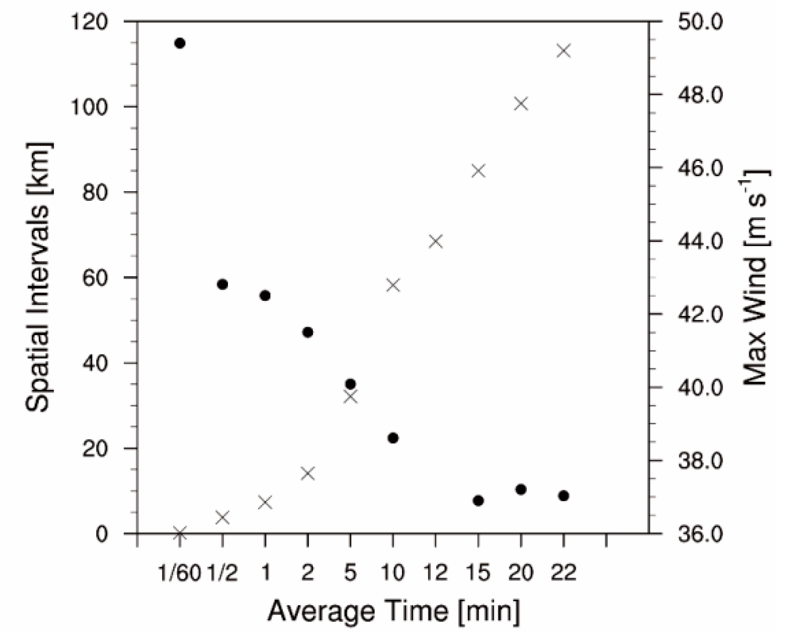
| avg. Time (Unit: minute) | 1/60 | 1/2 | 1 | 2 | 5 | 10 | 12 | 15 | 20 | 22 |
|---|---|---|---|---|---|---|---|---|---|---|
| u (unit: m s−1) | 0.53 | 1.36 | 1.63 | 2.08 | 3.27 | 4.48 | 5.68 | 6.10 | 7.27 | 8.38 |
| v (unit: m s−1) | 0.55 | 1.31 | 1.54 | 1.84 | 2.73 | 3.69 | 4.11 | 4.21 | 5.00 | 5.28 |
| t (unit: °C) | 0.08 | 0.25 | 0.33 | 0.44 | 0.77 | 0.98 | 1.25 | 1.48 | 1.93 | 1.57 |
| p (unit: hPa) | 0.80 | 1.82 | 2.39 | 3.51 | 6.69 | 8.54 | 12.11 | 15.46 | 20.74 | 18.22 |
| Exp. | Resolution of obs. (Temporal/Spatial) | QC Threshold | Substitution of obs. Error |
|---|---|---|---|
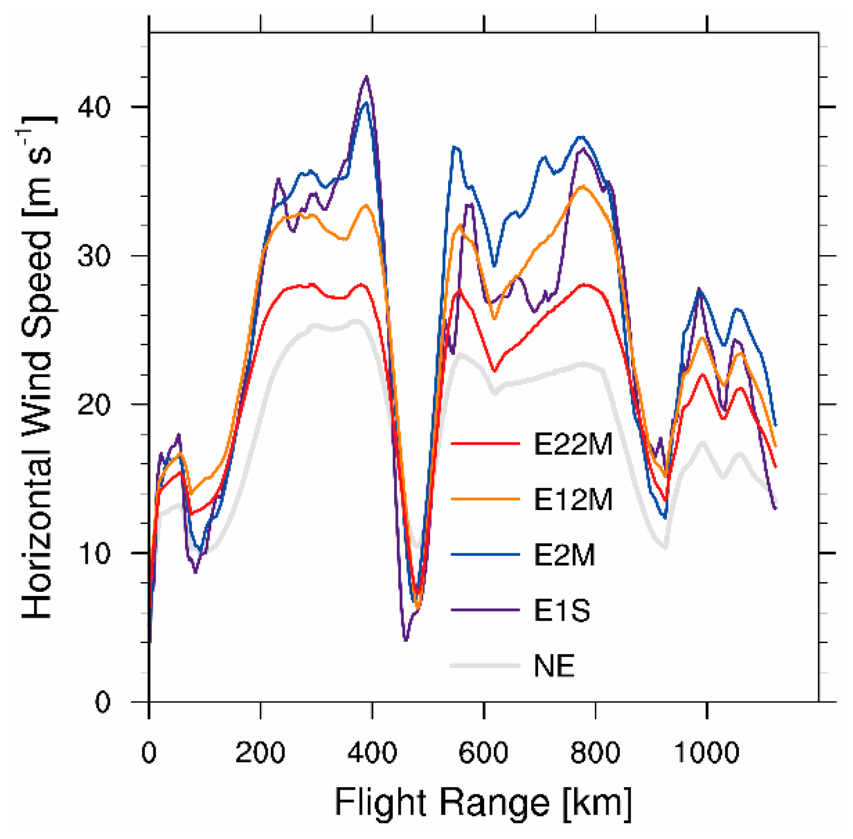
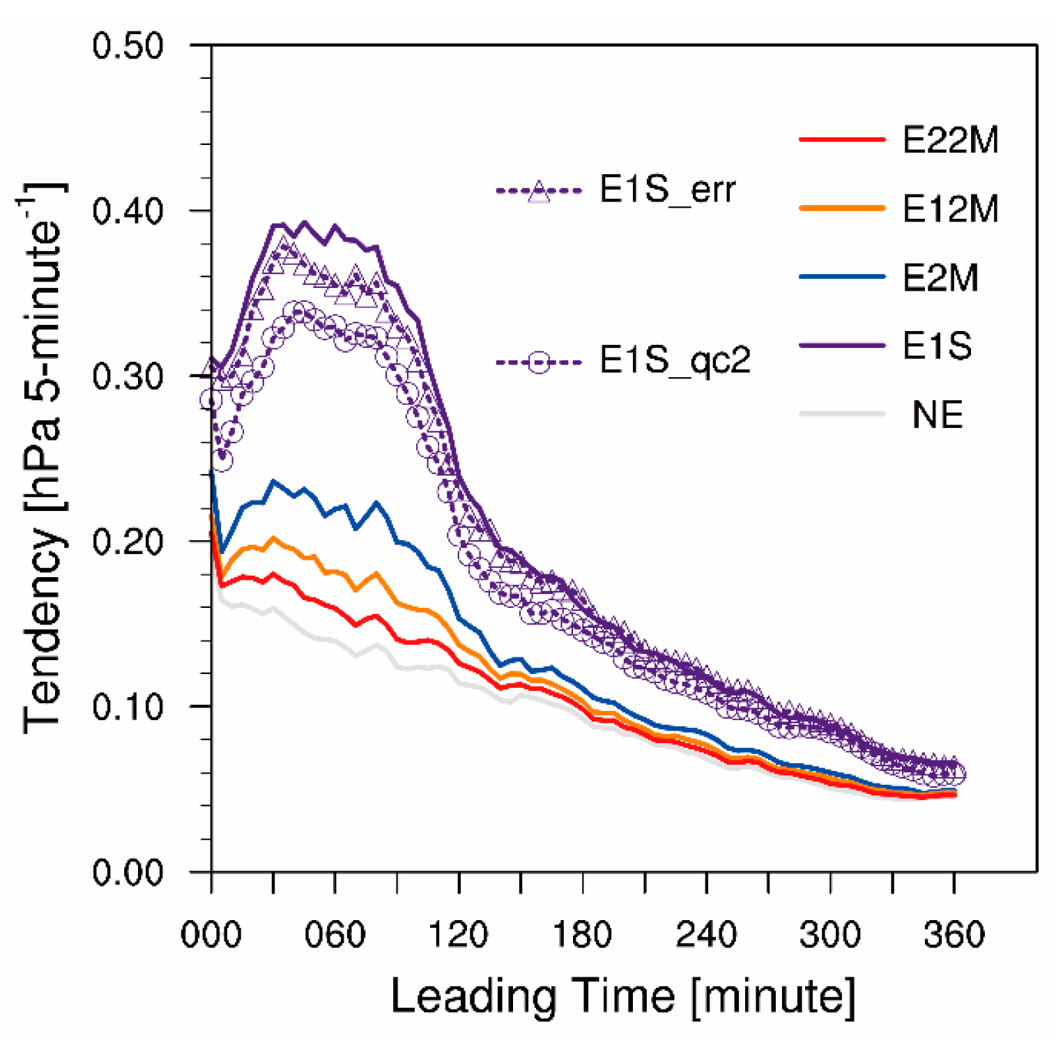
| NE | null | null | N |
| E1S | 1 s/0.12 km | 3.5 | N |
| E2M | 2 min/14.14 km | 3.5 | N |
| E12M | 12 min/68.47 km | 3.5 | N |
| E22M | 22 min/113.13 km | 3.5 | N |
| E1S_qc2 | 1 s/0.12 km | 2 | N |
| E1S_err | 1 s/0.12 km | 3.5 | Y (E22M) |
| Exp. | u (Unit: m s−1) | v (Unit: m s−1) | t (Unit: °C) | p (Unit: hPa) |
|---|---|---|---|---|
| NE | 8.20 | 8.84 | 3.10 | 3.54 |
| E1S | 4.36 | 5.22 | 3.82 | 5.95 |
| E2M | 3.78 | 3.74 | 2.78 | 2.45 |
| E12M | 4.89 | 4.32 | 2.96 | 2.60 |
| E22M | 6.35 | 6.27 | 3.06 | 2.84 |
| E1S_qc2 | 5.42 | 5.36 | 4.09 | 3.08 |
| E1S_err | 2.57 | 2.31 | 4.02 | 4.53 |
© 2019 by the authors. Licensee MDPI, Basel, Switzerland. This article is an open access article distributed under the terms and conditions of the Creative Commons Attribution (CC BY) license (http://creativecommons.org/licenses/by/4.0/).
Share and Cite
Gao, Y.; Xiao, H.; Jiang, D.; Wan, Q.; Chan, P.W.; Hon, K.K.; Deng, G. Impacts of Thinning Aircraft Observations on Data Assimilation and Its Prediction during Typhoon Nida (2016). Atmosphere 2019, 10, 754. https://doi.org/10.3390/atmos10120754
Gao Y, Xiao H, Jiang D, Wan Q, Chan PW, Hon KK, Deng G. Impacts of Thinning Aircraft Observations on Data Assimilation and Its Prediction during Typhoon Nida (2016). Atmosphere. 2019; 10(12):754. https://doi.org/10.3390/atmos10120754
Chicago/Turabian StyleGao, Yudong, Hui Xiao, Dehai Jiang, Qilin Wan, Pak Wai Chan, Kai Kwong Hon, and Guo Deng. 2019. "Impacts of Thinning Aircraft Observations on Data Assimilation and Its Prediction during Typhoon Nida (2016)" Atmosphere 10, no. 12: 754. https://doi.org/10.3390/atmos10120754
APA StyleGao, Y., Xiao, H., Jiang, D., Wan, Q., Chan, P. W., Hon, K. K., & Deng, G. (2019). Impacts of Thinning Aircraft Observations on Data Assimilation and Its Prediction during Typhoon Nida (2016). Atmosphere, 10(12), 754. https://doi.org/10.3390/atmos10120754