Article

Investigation of Transport and Transformation of Tropospheric Ozone in Terrestrial Ecosystems of the Coastal Zone of Lake Baikal

by
Alexander S. Zayakhanov
1,*,
Galina S. Zhamsueva
1,
Vadim V. Tcydypov
1,
Tumen S. Balzhanov
1,
Ayuna L. Dementeva
1 and
Tamara V. Khodzher
2
1
Institute of Physical Materials Science Siberian Branch, Russian Academy of Sciences, 670047 Ulan-Ude, Russia
2
Limnological Institute Siberian Branch, Russian Academy of Sciences, 664033 Irkutsk, Russia
*
Author to whom correspondence should be addressed.
Atmosphere 2019, 10(12), 739; https://doi.org/10.3390/atmos10120739
Submission received: 7 November 2019 / Revised: 12 November 2019 / Accepted: 20 November 2019 / Published: 25 November 2019
(This article belongs to the Section Air Quality)

Abstract

:
Forest ecosystems play an important role in the process of removing trace gases from the atmosphere. The purpose of this work is the experimental study of the flux and rate of the dry deposition of ozone on different types of vegetation in the Baikal region. Based on the eddy covariance method and the flux gradient methods (including the aerodynamic gradient method (AGM), the modified Bowen method (MBR) and modified gradient method (MGM)) and with experimental data, the quantitative estimates of the fluxes and dry deposition velocity of ozone on the underlying surface were obtained for different environments (grasslands, forest). The average values of the dry deposition velocity of ozone (Vd) were equal to 0.37 cm/s at night (0–3 h) and 0.91 cm/s during daytime hours (12–18 h). The ozone flux (F) was 0.24 μg m–2 s–1 at night and 0.72 μg m–2 s–1 in the afternoon. The quantitative estimates of Vd and F on vegetation and in the forest show a higher absorptive capacity of forests compared to soil vegetation.

1. Introduction

In recent years, the number of studies related to the influence of tropospheric ozone (O3) on the environment, both on a global and regional scale, has increased significantly. The increase of the concentration of nitrogen oxides, sulfur dioxide, and other trace gases leads to an increase of O3 at the ground level of the atmosphere due to photochemical reactions. Because these substances play an important role in changing the Earth's climate and affect living organisms and objects of the natural environment, observations of the O3 and components of the ozone cycle are included in the program of a special observation system, the Global Environment Monitoring System (GEMS) [1,2,3]. In Russia, regular monitoring observations of ground-level O3 are carried out, mainly at high-altitude stations and in areas with a temperate climate [3]. Unfortunately, experimental data are currently insufficient to obtain objective information about the spatial and temporal variations of surface ozone and other trace gases in an extreme continental climate; in particular, in the region of the Lake Baikal. Lake Baikal is a unique creation of nature. The lake was declared a UNESCO World Heritage Site in 1996 and included in the Man and the Biosphere Program. Primarily, the feature and uniqueness of Baikal are determined by the high strategic importance of the lake as the largest source of drinking water on the planet and as a reservoir with unique flora and fauna. Therefore, monitoring the condition and quality of the natural environment of Lake Baikal is an important task.
The anthropogenic impacts on the ecosystem of Lake Bikal are constantly growing due to the further development of industry in the region, and the expansion of tourist infrastructure and recreational areas in the coastal zone of the lake, which can lead to irreversible destructive processes. Another powerful source of pollutants into the atmosphere in Baikal region is forest fires. In regions located near Lake Baikal (Pribaikalia, Buryatia, and Transbaikalia), the tendency for climate warming is observed with a trend of annual air temperature increase of +1.3 °C over the next 100 years, twice the global temperature trend of +0.6 °C. [4]. In 2019, these three regions accounted for almost 30% of the total fires in Russia. Forests occupy up to 70% of the territory in this area, and are not only a large source of emissions of natural aerosols and gases, but also a sink for trace gases.
Ground-level ozone is a secondary pollutant of the atmosphere, the appearance of which in high concentrations indicates significant air pollution due to emissions of gases, namely ozone precursors. The increased concentrations of O3 may also be associated with the transfer of air masses from areas with a higher ozone content [3]. In this case, the role and relation of the photochemical and dynamic processes of the formation of O3 in many respects remain not yet fully understood. In some cases, photochemical processes are dominant processes, while in others they are dynamic processes, such as foehn phenomena [5], the influence of mountain valley circulation [6,7], and breeze phenomena [8]. All these features of the processes of O3 formation are noticeable in the Baikal region [9].
Within the framework of this problem, the role of terrestrial biosystems (natural ecosystems) in the process of the generation, transformation, and flux of trace gases remains underexplored. The role of terrestrial biota in the uptake and release of greenhouse gases (GHGs) has remained a controversial issue in modern environmental studies [10,11].
The results of numerous studies show the important role of forest ecosystems in the process of removing trace gases from the atmosphere [12,13,14,15,16]. The ozone uptake through the stomata is the primary pathway [17] of uptake responsible for plant injury by ozone. Inside leaves, ozone can be completely detoxified, but can also cause denaturation of membranes and the formation of free radicals, with a possible cascade of negative effects on the physiology and biochemistry of plants [18,19,20]. Dry deposition is an important process for the removal of O3, a phytotoxic air pollutant and greenhouse gas, which also plays a key role in the oxidizing ability of the atmosphere [21].
On the other hand, processes associated with atmospheric pollution have a negative impact on forest environments. The increased concentration of the pollutants in the atmosphere, such as sulfur dioxide, nitrogen oxides, ozone, heavy metals, and fluorides, has a diverse, oppressive effect on forest species, reduces the productivity of forests as a result of the interruption of photosynthesis and other physiological processes, worsens their condition, and in many cases leads to their desiccation [22,23]. Quantifying the atmospheric dry and wet deposition of trace gases is important for assessing their life expectancy in the air and their further potential impacts on different ecosystems. To quantify the flux of greenhouse gases to the underlying surface, the deposition rate and the flux are determined by the gradient method [24,25,26,27,28] or the eddy covariance (EC) [29].
In chemical transport models and monitoring networks, dry deposition is mostly estimated by parameters such as the dry deposition rate, which is calculated using an empirically developed dry deposition algorithms [29,30]. At the same time, the existing dry deposition algorithms have a large degree of uncertainty [31,32,33,34,35]. To reduce these uncertainties, experimental measurements of the field flux of trace gases are still needed. A large number of “field studies” have been performed on ozone dry deposition, mainly in the regions of the United States and Northern Europe [36,37,38,39]. These experimental data served as the basis for the development of parameterization schemes used in atmospheric models to describe the mechanisms of the dry deposition of greenhouse gases [29]. A number of more complex integrated schemes have been implemented in chemical models of atmospheric transport [40,41,42]. These models are parametrized on the basis of deposition flux measurements, but specific changing processes and pathways are still not fully understood, and their parameterization remains largely empirical.
The measurements of dry deposition fluxes of trace gases (O3, CO2, SO2, water vapor) mainly rely on micrometeorological methods [29]. Commonly, two types of methods are used: the turbulent pulsation method (eddy covariance, EC) and the flux gradient methods, including the aerodynamic gradient method (AGM) and the modified Bowen method (MBR). Eddy covariance is a direct measurement method that determines turbulent flux without any empirical assumptions [43,44]. This method is widely used for the estimation of the turbulent flux of carbon dioxide, sulfur dioxide, and ozone, such as in [45,46,47]. However, the use of the EC method is often limited by the complexity of quality measurements at sufficiently high frequencies to resolve the covariance between turbulent vertical wind speed and scalar concentration fluctuations [48].
In recent years, a new modified micrometeorological gradient method has been developed to quantify the dry deposition of ozone, carbon dioxide, sulfur dioxide, and nitrogen oxides over the forest canopy using concentration gradients at levels above and below the top of the forest canopy (modified gradient method—MGM) [28]. The MGM method gives values of fluxes and rates of dry deposition almost as a measurement of eddy covariance. This approach of the flux gradient theory is used in our investigation as an alternative method for determining the flux of O3 to the underlying surface. The global network of micrometeorological sites (masts) is used to monitor the exchange of greenhouse gases between the biosphere and the atmosphere. Currently, the FluxNet network includes about 700 stations [49], which cover all climatic zones and almost all types of global vegetation. At present in Russia, such studies have been started recently at several points in the European part of the country, as part of the development of a regional environmental monitoring system for greenhouse gas emissions, named RusFluxNet [50]. The results of these studies are not always be applicable to the natural and climatic conditions of the Baikal region, as it has a wide variety of vegetation types in its territory.
For the Baikal region, the environmental problems of air pollution and biodiversity conservation is of great importance. Woodlands occupy a significant part of the coastal zone of Lake Baikal. In the Baikal region, a breeze phenomenon plays an important role in the circulation processes of air mass transfer. Constant air exchange occurs between the land and water surface. Polluted air masses from the lake affect and influence forest vegetation for a long time in day breeze conditions [9]. The industrial centers (Irkutsk, Angarsk, Shelekhov, and Cheremkhovo) are situated in areas of atmospheric influence on Lake Baikal. With the predominant south-western transport of air masses, the emissions from these centers are transferred to the water area of the lake region. Forest fires are an additional source of pollutants in the region. Anthropogenic impacts on the ecosystem of Lake Baikal are constantly growing due to the further development of industry in the region, and the expansion of tourist infrastructure and recreational areas in the coastal zone of the lake, which can lead to irreversible destructive processes.
The contribution of forest vegetation to the uptake of aerosol and trace gases, such as О3, NOx, SO2, and СО2, is high during the daytime, when turbulent processes and the photosynthetic activity of plants are activated. Such focused research in the Baikal region has not yet been conducted. Regarding the increasing anthropogenic load, extreme natural phenomena such as forest fires and the assessment of environmental damage to the ecosystem of Lake Baikal still remains an unsolved problem due to the lack of observational data. There are insufficient data on observations of the composition of chemically active trace gases, aerosols, and the inclusion of various factors affecting the composition and quality of atmospheric air, including uptake and emission of impurities in natural ecosystems (forest, grass, water).
The purpose of this study is to present new results of the quantitative estimates of the fluxes of O3 and the rate of dry deposition of ozone on grasslands and in the forest in the Baikal region, based on approved calculation methods and experimental data. The results of the measurements of ozone exchange processes between the atmosphere and the underlying surface are presented.

2. Experiments

A method of gradient measurements regarding the concentration of ozone and atmospheric dynamic characteristics with the help of meteorological masts was used to study the effect of the thermal stratification of the atmosphere on O3, and to study the characteristics of the exchange processes of trace gases (fluxes and rates of dry deposition) between the atmosphere and the underlying surface (grasslands, forest).
The sample site is located within the territory of the scientific station, which is situated at a distance of 500 m from the Baikal water area, at heights of 60 m from the lake level. Air samples were taken at different heights above ground level using Teflon tubes. Observations were performed using chemiluminescent gas analyzers 3-02 P-А for ozone (OPTEK Corp., St. Petersburg, Russia). The relative error of chemical measurements did not exceed ±20%. The lower detectable limit was 1 μg m–3, and the response time was 30 s. The calibration of gas analyzers was carried out automatically by means of the built-in calibrated sources of microstreams; besides controlling the measurement error, the gas analyzers were calibrated against a Mod. 8500 Monitor Labs instrument (Teledyne Monitor Labs, Englewood, CO, USA). Simultaneously, at these same heights, the meteorological and turbulent parameters of the atmosphere were measured using the acoustic meteorological complexes: AMK-03 and EXMETEO (Sibanalitpribor Ltd., Tomsk, Russia). The meteorological complex provides information on instantaneous values of wind velocity (in three mutually perpendicular directions) and air temperature and carries out the measurements at frequencies from 10 to 160 Hz, followed by an automatic calculation of up to 60 statistical and turbulent parameters of the atmosphere, and in particular, lapse rates (based on the Monin–Obukhov similarity theory; software developed in the Institute of Monitoring of Climatic and Ecological Systems, Siberian Branch, Russian Academy of Sciences, Tomsk, Russia). The 10 min average lapse rates were calculated by sampling from the corresponding temperature set, followed by processing to remove separate bursts beyond the (95%) confidence interval.

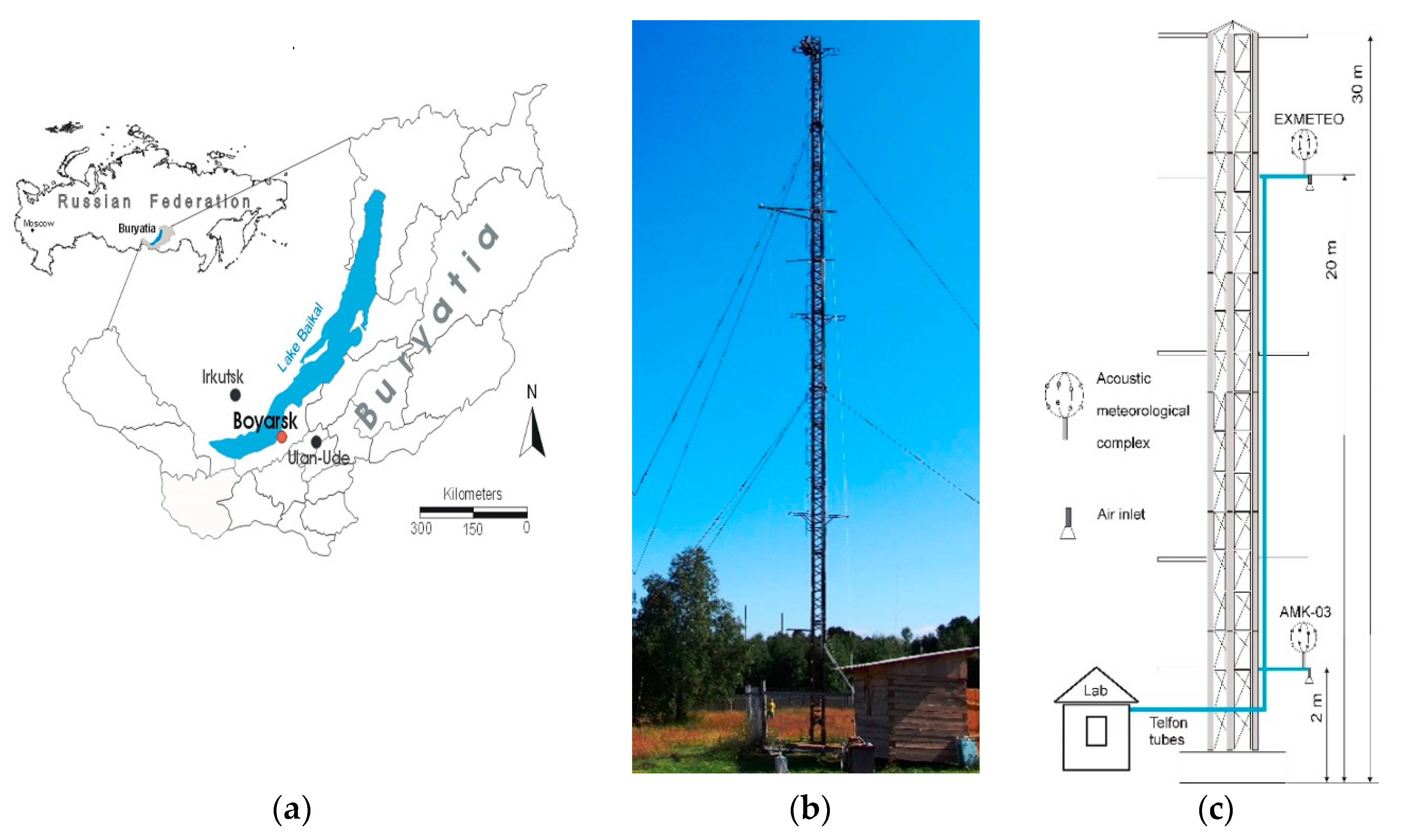
2.1. Atmosphere Experiments—Grasslands

In the summer period 2018 (July 12–August 23), experimental investigations of ozone exchange processes between the atmosphere and the underlying surface (grasslands) were carried out.
The gradient measurements of O3, meteorological parameters, vertical fluxes of heat and moisture, and dynamic characteristics of the atmosphere at the Boyarsky stationary site (51°83′ N, 106°06′ E) of Institute of Physical Materials Science Siberian Branch, Russian Academy of Sciences, were carried out using a 30 m meteorological mast and automated system for monitoring atmospheric pollution. The scientific station is situated 160 km from Ulan-Ude on the southeastern coast of Lake Baikal, in a village with a developed transport and communications infrastructure (Figure 1a).
Air samples were taken at two heights (2 and 20 m above ground level) to determine the concentration of O3 (Figure 1c).
To estimate the flux of ozone to the underlying surfaces, the calculations were conducted with proven methods [51,52,53]. To evaluate the flux of ozone to the underlying surfaces as a quantitative characteristic, the velocity and deposition rate of ozone are used (Equation (1)):
F = −Vd × C
where C is the concentration of O3 and Vd is the dry deposition velocity.
The dry deposition velocity is calculated by analogy with Ohm's law, considering different types of resistance to the transfer of pollutants from the atmosphere to the underlying surface [51]. The dry deposition velocity for gases is the following:
Vd = 1/(Ra + Rb + Rc)
where Ra is the aerodynamic resistance to the flux of gases, Rb is the quasi-laminar sublayer resistance, and Rc is the canopy resistance [52].
Under conditions of a stable atmosphere in which breeze phenomena are formed, the resistance Ra (Equation (3)) and friction velocity u* (Equation (4)) are determined according to [53], and the resistance Rb is determined according to Equation (5) [51]:
Rb = (1/ku) × (Pr (ln((Zr − d)/Z0h) + (βh/L) × (Zr − d − Z0h))
u* = k × Ur × (ln ((Zr − d)/Z0m) + (βh/L) × (Zr − d − Z0m))−1
Rb = (2/ku)× (Sc/Pr)2/3
where u* is the friction velocity, Pr is the Prandtl number, Sc is the Schmidt number, Zr is the measuring height, k equals 0.4 (the Karman constant), d is the displacement height, Z0h is the roughness parameter for energy, Z0m is the roughness parameter for momentum, βm and βh are empirical constants, Ur is the horizontal wind speed at a given height, and L is the Monin-Obukhov scale.

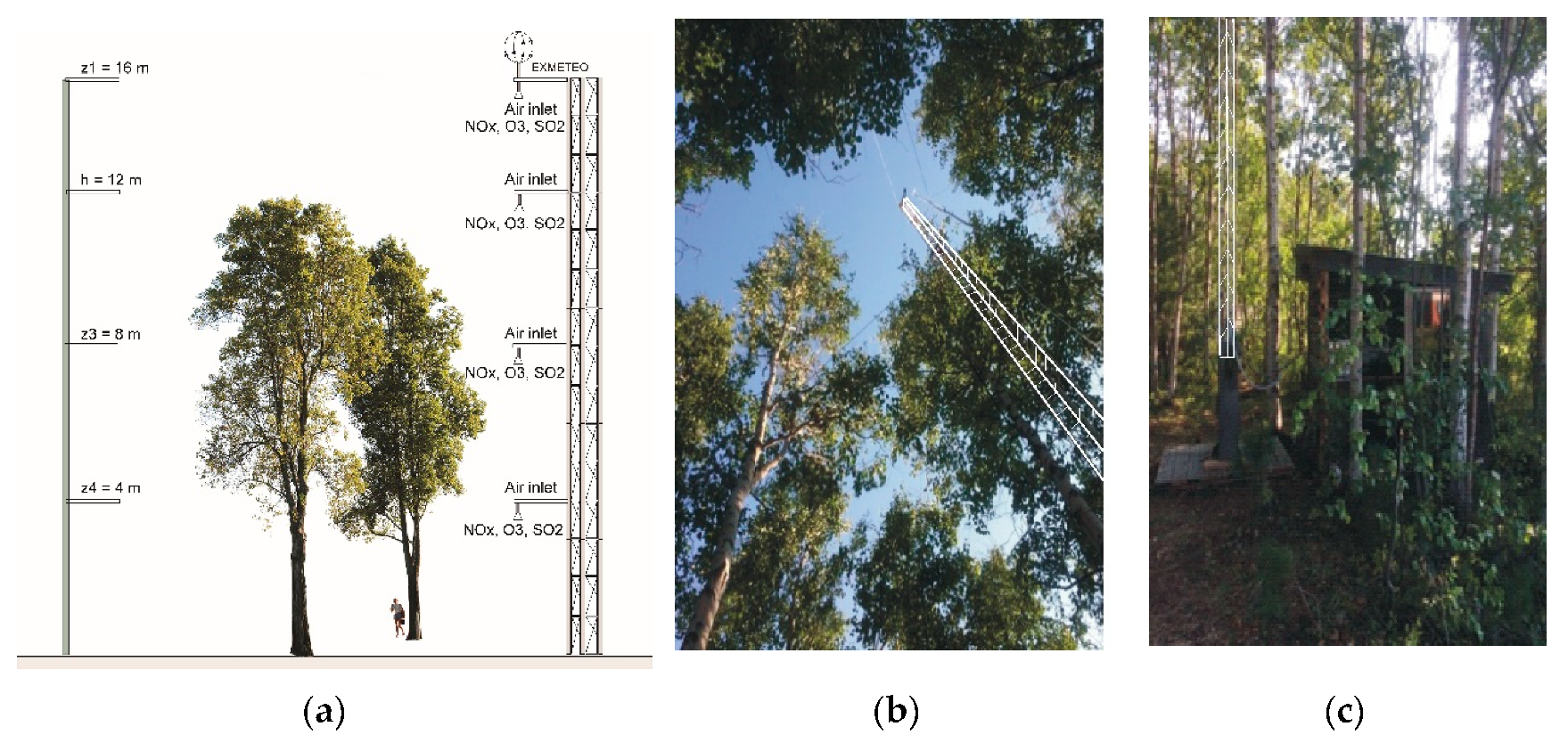
2.2. Atmosphere Experiments—Forest

A measuring platform was prepared to organize the experiments on the study of gas exchange between the atmosphere and forest vegetation in the coastal zone of Lake Baikal in the summer period 2018 (August 5–23). On this platform, a meteorological mast (16 m) was installed. Using the meteorological mast, gradient measurements of meteorological parameters, pulse characteristics of temperature, wind speed, and concentrations of O3 at four heights levels above and below the forest canopy were carried out (Figure 2).
The forest is on average 40–50 years old and consists of birch, larch, pine, and cedar. The birch trees had an average crown height 12 m with a leaf area index (LAI) peak of 5.9, and mainly grew near the meteorological mast, within a radius of 50 m. The measurements were carried out in a mixed forest, which had a predominance of Erman birch, Siberian cedar, and ordinary pine. The forest is quite dense, and trees are located on average at a distance 2 m.
LAI was determined by the results of the digital processing of hemispherical photos [54].
Using results of measurements of meteorological parameters, such as turbulent characteristics of temperature, wind speed, and concentration O3 at different heights, the calculations of the dry deposition velocity of ozone were conducted based on MGM [28]. Applying the flux gradient theory inside the canopy of the forest, the flux F (z) can be calculated as in Equation (6), and the remaining parameters are calculated using Equations (7)–(9):
F = − Kc (z) dC/dz
where Kc(z) is the vortex diffusion and dC/dz is the vertical gradient of the gas concentration.
F = (C (z1) – C (z3))/(Ra (z1/h) + Ra (h/z3))
Ra (z1/h) = (ku*)−1 [ln (z1 − d)/(h − d)+ Ψh ((z1 − d)/L) − Ψh ((h − d)/L)]
d = h (0.1 + LAI0.2/2)
z0 = h (0.215 − LAI0.25/2)
where z1 > h; z3 < h, k is the Karman constant, C (z1) and C (z3) are concentrations of О3 at heights z1 and z3, Ra (z1/h) is the aerodynamic resistance to flux, Ψh and Ψm are the integrated heat stability correction function, u and w are the horizontal and vertical wind speeds, u* is the friction velocity, L is the Monin-Obukhov scale, h is the height of the tree crown (the height of the canopy), z0 is the roughness length, and d is the displacement height.
The aerodynamic resistance at heights z3 < h (inside of trees crown) is calculated by Equation (11):
Ra(h/z3) = ∫z3h(dz/(Kc(z)*)
According to [46], the vertical diffusion coefficient is Kc(z) calculated by Equation (12):
Kc (z) = 0.8 ((∫0zCm (z) a (z) u (z)2 dz))/(dU (z)/dZ)
Cm (z) = (u*2 h)/(LAI ∫0hU (z) dZ)
where Cm(z) is the effective resistance coefficient, a (z) is the density of the sheet area at height z, and U(z) is the wind speed at height z.
Using Equation (14) [55], the wind speed profile within the canopy is determined:
U (z) = U (h)*e−α(1−z/h) = U (z1) ((ln (h − d) ‒ ln (z0m) + Ψm (((h − d)/L)) − Ψm [(z0m/L)])/(ln (z1 − d) ‒ ln(z0m) + Ψm [((z1 − d)/L)] − Ψm [(z0m/L)])*e(−α(1−z/h))
where U(z) is the wind speed at height z and z0m is the roughness length for momentum.
For a stable atmosphere:
u* = (kU (z1))/(ln (z1 − d)/zom) + (βm/L) (z1 − d − zom); (z1 − d)/zom ≥ 0
For an unstable atmosphere:
u* = (kU (z1))/ln ((1 − γm (z1 − d)/L)1/4 − 1)/((1 − γm (z1 − d)/L)1/4 + 1) − ln ((1 − γm (zom/L))1/4 − 1)/((1 − γm zom/L)1/4 + 1) + 2 tan−1 (1 − γm (z1 − d)/L)1/4 − 2 tan−1(1 − γm (z1 − d)/L)1/4); (z1 − d)/zom ≥ 0
where βm = 6.0; γm = 19.3; zom = 1 [56].

3. Results and Discussion

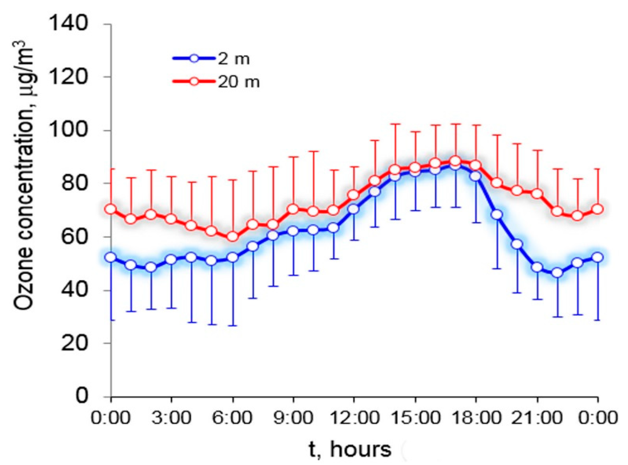
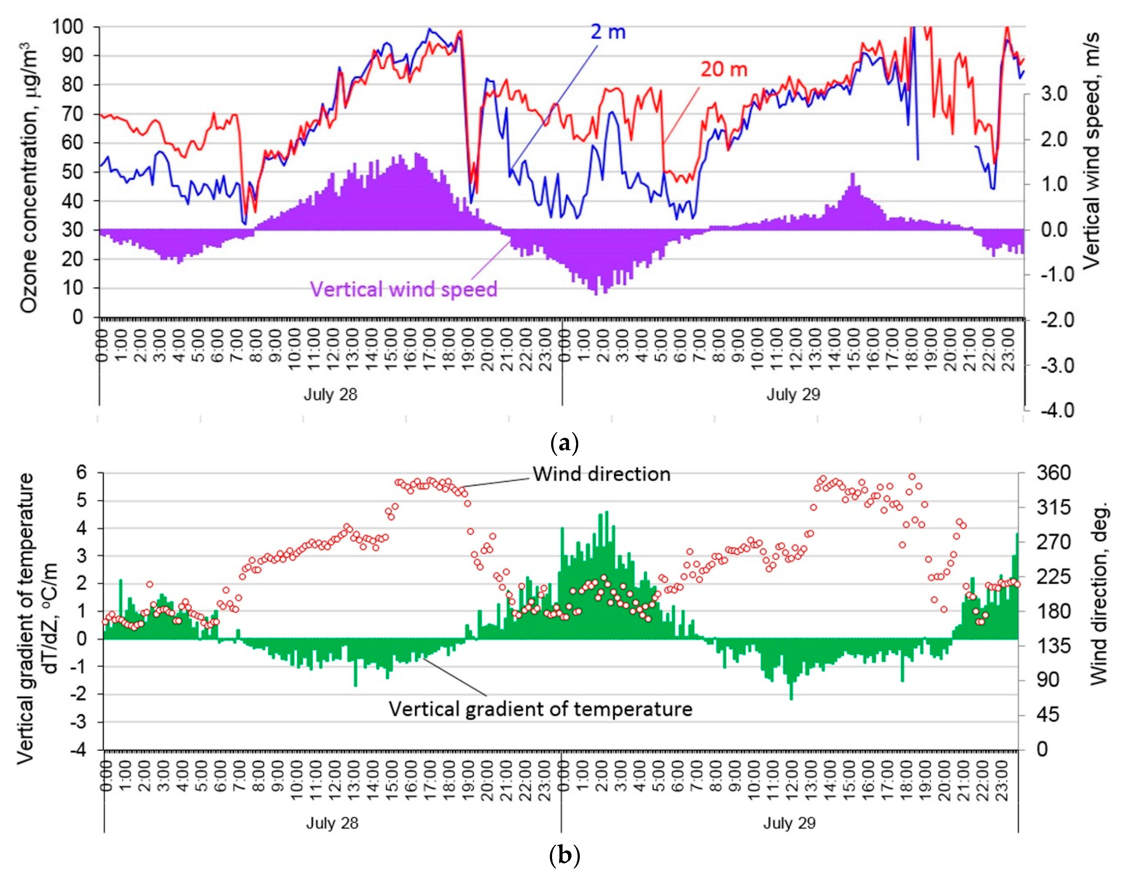
3.1. Gradient Measurements of Ozone

Figure 3 presents the diurnal variations in hourly average values of O3 at heights of 2 and 20 m for all periods of observation. The diurnal ozone variations strongly differ between the near-surface (2 m) and near-ground (20 m) layers, where the effect of the underlying surface is markedly weaker. The diurnal О3 behavior at high heights (20 m) is smoother than near the ground (2 m). In evening and night hours, the largest differences are observed. The ozone concentrations at different heights become equal in daytime as the temperature rises, and turbulent processes intensify in the near-ground atmospheric layer. As a rule, after sunset and night hours with a weak wind and the absence of UV illumination, the concentration of O3 is higher at the upper level than at the lower level. This distribution of ozone corresponds to weak air mixing due to the occurrence of temperature inversions and the dominant role of O3 uptake by the underlying surface.
Figure 4 shows in more detail the results of synchronous measurements of O3 as a function of the temperature gradient and wind direction at different heights on July 28 and 29, 2018, as the most typical conditions of breeze formation.
In morning hours, as the Earth’s surface is heated, convective flows are generated and lead to a breakup of the near-ground inversion and intensification of turbulent processes (Figure 4b), giving rise to a gradual growth and equalizing the ozone concentration at different heights (Figure 4a). In these hours, there is a reversal of wind direction, with the coastal breeze switching to a daytime breeze blowing from the lake. At evening time, after the sunsets and the soil temperature decreases, temperature inversions form in the near-ground atmospheric layer (Figure 4b) and turbulent processes become less intense. Moreover, downdrafts at heights of 20 m maintain a higher concentration of О3, supplied from above the canopy (Figure 4a). Figure 4a shows the vertical wind speed (w). The negative values of w indicate the flow direction from top to bottom. The ozone concentration rapidly decreases by dry deposition on the underlying surface in the absence of vertical exchange, especially in the lowermost near-surface layer (2 m).

3.2. Flux of Ozone to the Underlying Surface

The values of L and Ur are determined from the data of pulsation measurements of wind speed and temperature using acoustic meteorological complexes. According to [29,57], the following characteristics are used for calculation: PrSc ≈ 0.95; βm = 6,0; βh = 7.8; Z0m= 0.05; d= 0.4 cm. The surface resistance of Rc is determined on the basis of the experimental data and results [57].
According to Equations (1)–(4), the velocity and fluxes of ozone dry deposition at night (0–3 h) and during the day (12–18 h) in the conditions of breeze circulation observed on July 28–29 were determined (Table 1).
At night in the atmosphere, the velocity of the dry deposition of O3 and its flux to the underlying surface are much lower than in the daytime in periods when turbulent processes are less intense. In the daytime, the processes of O3 formation dominate over the processes of its destruction, as evidenced by the increase of O3 in the daytime. At night, in the absence of UV illumination, the generation process stops and forests act as a sink for ozone.
Figure 5 shows the gradient ozone concentration between levels of 8–12 m. Ozone concentration is minimal in the morning (40 µg/m3), maximum values are observed during the day (up to 90 µg/m3), and then О3 decreases at night. Gradients between the two heights in the morning are minimal and amount to 1.5 µg/m3 at 11 h compared with other periods of the day (Figure 5). The most efficient turbulent air exchange is noted between the layer above the top of the forest and the layer inside the tree canopy. During such a turbulent exchange, the concentration gradients of O3 are significantly reduced. It should be noted that the effects of chemistry on the О3 flux are small, probably because the chemical reactions for О3 have longer time intervals than the turbulent exchange [39,44]. Differences in meteorological conditions (temperature, wind speed, humidity, etc.) during the daytime and at night have a significant influence on the concentration and deposition rate of О3.
Figure 6 shows the dependence of ozone concentration on heights during the daytime and nighttime. Ozone concentrations at 15 m are greater than at 8 m and 4 m. High concentrations of O3 were noted, especially at heights above the canopy of forest vegetation (15 m). This feature characterized the behavior of O3 near the coastal zone of Lake Baikal [9]. A similar feature of ozone is noted in [58,59], where authors explained the relatively high level of O3 by the following reasons: (1) air mass recirculation caused by nighttime sea breeze, which, with the onset of the night breeze, transfers the aged air masses enriched with O3 from the mainland to the coastline at night and in the morning; (2) subsidence of air masses rich in O3 at the level of the middle troposphere; (3) a decrease in the height of the boundary layer. The values of the concentration gradient at different heights indicate that the precipitation and uptake of О3 actually occur directly under the forest canopy, due to uptake to the underlying surface.
In Table 2, parameters and values for the calculation of fluxes and the dry deposition rates of О3 are presented.
The meteorological parameters of the atmosphere were measured using the acoustic meteorological complex EXMETEO, the Monin–Obukhov length scale (L).
The results of the calculation of daily cycles of Vd and F are shown in Figure 7. The dry deposition rate averaged about 0.4 cm/s during the night and reached a daily maximum of 1 cm/s in the afternoon hours (Figure 7a). The flux of O3 in the forest during the experiments at night and early morning hours averaged 0.2 µg m2 s−1; the maximum value was observed during the daytime (15–16 h) at 0.8 µg m2 s−1.
The calculations were carried out using the software system Mathcad 15 (Parametric Technology Corporation, Boston, MA, USA). The average values of the dry deposition velocity of O3 were equal to 0.37 cm/s at night (0–3 h) and 0.91 cm/s during daytime hours (15–18 h). The ozone flux was 0.24 µg m2 s–1 at night and 0.72 µg m2 s–1 in the afternoon. For the forest environment, the average values of the dry deposition velocity of O3 and flux of O3 are presented in Table 3.
The quantitative estimates of Vd and F on grasslands (Table 1) and in the forest (Table 3) show a higher absorptive capacity of forests compared to soil vegetation.
Similar data of the dry deposition velocity of ozone were obtained in experiments above canopies of deciduous forest [60] and mixed deciduous forest [61] for daytime and nighttime. In [28], different methods for determining the dry deposition rate of O3 (AGM, MBR, MGM, EC) in Harvard Forest were compared. Although the trends were similar, the MBR and AGM gave higher values of Vd than the EC method. According to EC, the value of Vd was equal 0.2 cm/s during the night and reaching a daily maximum of 0.54 cm/s around noon. Vd according to the MBR and AGM methods reached about 0.8 and 1.3 cm/s during the daytime, respectively, and about 0.4 cm/s remained during the night. The MGM Vd value was in good agreement with EC Vd in the daytime, but was slightly higher at night. It was discovered that the EC methodology underestimates the flow during quiet nighttime periods in the Harvard Forest. According to earlier studies conducted in Harvard deciduous forest (1990–1994), dry deposition rates for daytime during the summer reach up to 0.8 cm/s, while during the nighttime reach 0.2 cm/s [26].
The results of experiments studying the deposition rate and ozone flows above grasslands in the Baikal region is consistent with the results of [62], which were carried out in the framework of the European Union environmental research program, integrated into the Surface Resistance Emergency Measurements Program (SREMP). From the results of [62], during the summer period the dry deposition velocity of ozone was equal to 0.3–0.4 cm/s in daytime, while during nighttime was 0.1 cm/s. Maximum daytime ozone flux was 0.4–0.5 µg m2 s−1. According to preliminary estimates, the dry deposition is equal 20–25% of total O3 from the troposphere [63,64]; the rate of dry deposition of ozone tends to be higher in vegetation than on surfaces without vegetation [29]. Recent studies have clearly shown that field measurements of O3 deposition can significantly improve our ability to more accurately represent dry O3 deposition in vegetation using modeling techniques [65,66,67].

4. Conclusions

In this study, to quantify the flux of O3 to the underlying surface in the Baikal region, the deposition velocity and flux of ozone values were used. For different environments (grasslands, forest) in the Baikal region, the quantitative estimates of the fluxes and rates of dry ozone deposition on the underlying surface were obtained. These preliminary assessment results were carried out based on the proven calculation methods and experimental data.
For the forest environment, the average values of the dry deposition velocity of O3 were equal to 0.37 cm/s at night (0–3 h) and 0.91 cm/s during daytime hours (12–18 h). The ozone flux was 0.24 μg m−2 s−1 at night and 0.72 μg m−2 s−1 in the afternoon. In grasslands, the dry deposition velocity of O3 and the flux of O3 did not exceed 0.16 cm/s and 0.08 μg m−2 s−1 at night and 0.34 cm/s and 0.21 μg m−2 s−1 during daytime. The quantitative estimates of the Vd and F on grasslands and in the forest showed the higher absorptive capacity of forests compared to grasslands.

Author Contributions

Conceptualization, A.S.Z. and G.S.Z.; methodology, A.S.Z. and G.S.Z.; software, V.V.T. and A.L.D.; statistical analysis, T.S.B. and A.L.D.; validation, A.S.Z. and G.S.Z.; formal analysis, A.S.Z. and G.S.Z.; investigation, A.L.D., V.V.T., and T.S.B.; resources, A.S.Z. and G.S.Z.; writing—original draft preparation, A.S.Z. and G.S.Z.; writing—review and editing, A.S.Z., G.S.Z., and V.V.T.; visualization, A.S.Z. and V.V.T.; supervision, A.S.Z.; project administration, G.S.Z. and T.V.K.; funding acquisition, G.S.Z. and T.V.K.

Funding

This research was funded by the Russian Foundation for Basic Research (RFBR) (grant No. 18-45-030032 r_a). The desk-based processing of experimental data and numerical calculations was carried out with the support of the Russian Science Foundation (RSF) (grant No. 19-77-20058). The measurements of meteorological parameters of the atmosphere were conducted by the meteorological complex of the Center for Collective Use of Scientific Equipment, “Atmosphere”, of the V.E. Zuev Institute of Atmospheric Optics of the Siberian Branch of the Russian Academy of Science (IAO SB RAS).

Conflicts of Interest

The authors declare no conflict of interest.

References

  1. Perov, S.P.; Khrgyaan, A.K.H. Current Problems of Atmospheric Ozone, 3rd ed.; Hydromet: Leningrad, Russia, 1980; pp. 134–156. [Google Scholar]
  2. Treshou, M. Air Pollution and Plant Life, 3rd ed.; Hydromet: Leningrad, Russia, 1988; pp. 356–360. [Google Scholar]
  3. Belan, B.D. Ozone in the Troposphere; Institute of Atmosphere Optics SB RUS: Tomsk, Russia, 2010; p. 487. (In Russian) [Google Scholar]
  4. Shimarev, M.N.; Kuimova, L.N.; Sinyokovich, V.N.; Tsekhanovskiy, V.V. On the manifestation on Baikal of global climate change in the twentieth century. Dokl. Ran 2002, 383, 397–400. [Google Scholar]
  5. Demin, V.I.; Beloglazov, M.I.; Mokrov, E.G. Foehn effects above Khibiny in changes of surface ozone concentration. Atmos. Ocean. Opt. 2005, 18, 613–617. [Google Scholar]
  6. Demin, V.I.; Beloglazov, M.I. On the influence of local circulation processes on surface ozone dynamics. Atmos. Ocean. Opt. 2004, 17, 331–333. [Google Scholar]
  7. Zayakhanov, A.S.; Zhamsueva, G.S.; Tsydypov, V.V.; Balzhanov, T.S. Results of monitoring or surface ozone in atmosphere of Ulan-Ude. Meteorol. Hydrol. 2013, 12, 76–84. [Google Scholar] [CrossRef]
  8. Zayakhanov, A.S.; Zhamsueva, G.S.; Tsydypov, V.V.; Balzhanov, T.S. The influence of dynamic processes on the variations of ozone and other small gas impurities near the coastal zone of Lake Baikal. Atmos. Ocean. Opt. 2015, 28, 505–511. [Google Scholar]
  9. Zayakhanov, A.S.; Zhamsueva, G.S.; Tsydypov, V.V.; Balzhanov, T.S. Daily dynamics of ozone and other small gas impurities in the coastal zone of Lake Baikal (station Boyarsky). Meteorol. Hydrol. 2017, 8, 85–92. [Google Scholar]
  10. Clark, D.A.; Clark, D.B. Assessing tropical forests climatic sensitivities with longterm data. Biotropica 2011, 43, 31–40. [Google Scholar] [CrossRef]
  11. Stocker, T.F.; Qin, D.; Plattner, G.K.; Tignor, M.; Allen, S.K.; Boschung, J.; Midgley, B.M. Сlimate Change 2013: The Physical Science Basis. Contribution of Working Group I to the fifth Assessment Report of the Intergovernmental Panel on Climate Change; Cambridge University Press: Cambridge, UK; New York, NY, USA, 2013. [Google Scholar]
  12. Malhi, Y.; Baldocci, D.D.; Jarvis, P.G. The carbon balance of tropical, temperate and boreal forests. Plant Cell Environ. 1999, 22, 715–740. [Google Scholar] [CrossRef]
  13. Falge, E.; Tenhunen, J.; Baldocchi, D.; Aubinet, M.; Bakwin, P.; Berbigier, P.; Bernhofer, C.; Bonnefond, J.M.; Burba, G.; Clement, R.; et al. Phase and amplitude of ecosystem carbon release and upt ake potentials as derived from FLUXNET measurements. Agric. For. Meteorol. 2002, 113, 75–95. [Google Scholar] [CrossRef]
  14. Granados, J. Tropical Forest Response to Climate Change; Springer: Berlin/Heidelberg, Germany, 2006. [Google Scholar]
  15. Rudnev, N.I. The Environment-Forming Role of Vegetation in Tropical and Temperate Latitudes of Eurasia; Institute of Ecology and Evolution RUS: Moscow, Russia, 2003; p. 32. (In Russian) [Google Scholar]
  16. Luyssaert, S.; Schulze, E.D.; Borner, A.; Knohl, A.; Hessenmoller, D.; Law, B.E.; Ciais, P.H.; Grace, J. Old-growth forests as global carbon sinks. Nature 2008, 455, 213–215. [Google Scholar] [CrossRef]
  17. Loreto, F.; Fares, S. Is ozone flux inside leaves only a damage indicator? Clues from volatile isoprenoid studies. Plant Physiol. 2007, 143, 1096–1100. [Google Scholar] [CrossRef] [PubMed]
  18. Pell, E.J.; Schlagnhaufer, C.D.; Arteca, R.N. Ozone-induced oxidative stress: mechanisms of action and reaction. Physiol Plant. 1997, 100, 264–273. [Google Scholar] [CrossRef]
  19. Olofsson, J.; Oksanen, L.; Oksanen, T.; Tuomi, M.; Hoset, K.S.; Virtanen, R.; Kyrö, K. Long-Term Experiments Reveal Strong Interactions between Lemmings and Plants in the Fennoscandian Highland Tundra. Ecosystems 2014, 17, 606–615. [Google Scholar] [CrossRef]
  20. Laysk, A.K. Kinetics of C3 Plant Photosynthesis; Nauka: Moscow, Russia, 1991; p. 22. [Google Scholar]
  21. Finlayson-Pitts, B.J.; Pitts, J.N. Chemistry of the Upper and Lower Atmosphere. Theory, Experiments, and Application; Academic Press. Elsevier Inc.: London, UK, 2000; p. 993. [Google Scholar]
  22. Braun, S.; Schindler, C.; Rihm, B. Growth losses in Swiss forests caused by ozone: Epidemiological data analysis of stem increment of Fagus sylvatica L. and Picea abies Karst. Environ. Pollut. 2014, 192, 129–138. [Google Scholar] [CrossRef] [PubMed]
  23. Juráň, S.; Edwards-Jonášová, M.; Cudlín, P.; Zapletal, M.; Šigut, L.; Grace, J.; Urban, O. Prediction of ozone effects on net ecosystem production of Norway spruce forest. iForest 2018, 11, 743–750. [Google Scholar] [CrossRef]
  24. Meyers, T.P.; Hall, M.E.; Lindberg, S.E.; Kim, K. Use of the modified Bowen-ratio technique to measure fluxes of trace gases. Atmos. Environ. 1996, 30, 3321–3329. [Google Scholar] [CrossRef]
  25. Park, J.H.; Fares, S.; Weber, R.; Goldstein, A.H. Biogenic volatile organic compound emissions during BEARPEX 2009 measured by eddy covariance and flux-gradient similarity methods. Atmos. Chem. Phys. 2014, 14, 231–244. [Google Scholar] [CrossRef]
  26. Munger, J.W.; Wofsy, S.C.; Bakwin, P.S.; Fan, S.M.; Goulden, M.L.; Daube, B.C.; Goldstein, A.H.; Moore, K.E.; Fitzjarrald, D.R. Atmospheric deposition of reactive nitrogen oxides and ozone in a temperate deciduous forest and a subarctic woodland: 1. Measurements and mechanisms. J. Geophys. Res. 1996, 101, 12639–12657. [Google Scholar] [CrossRef]
  27. Urbanski, S.; Barford, C.; Wofsy, S.; Kucharik, C.; Pyle, E.; Budney, J.; McKain, K.; Fitzjarrald, D.; Czikowsky, M.; Munger, J. Factors controlling CO2 exchange on timescales from hourly to decadal at Harvard Forest. J. Geophys. Res. 2007, 112. [Google Scholar] [CrossRef]
  28. Wu, Z.Y.; Zhang, L.; Wang, X.M.; Munger, J.W. A modified micrometeorological gradient method for estimating O3 dry depositions over a forest canopy. Atmos. Chem. Phys. 2015, 15, 7487–7496. [Google Scholar] [CrossRef]
  29. Wesely, M.; Hicks, B. A review of the current status of knowledge on dry deposition. Atmos. Environ. 2000, 34, 2261–2282. [Google Scholar] [CrossRef]
  30. Pleim, J.; Ran, L. Surface flux modeling for air quality applications. Atmosphere 2011, 2, 271–302. [Google Scholar] [CrossRef]
  31. Flechard, C.R.; Nemitz, E.; Smith, R.I.; Fowler, D.; Vermeulen, A.T.; Bleeker, A.; Erisman, J.W.; Simpson, D.; Zhang, L.; Tang, Y.S.; et al. Dry deposition of reactive nitrogen to European ecosystems: a comparison of inferential models across the NitroEurope network. Atmos. Chem. Phys. 2011, 11, 2703–2728. [Google Scholar] [CrossRef]
  32. Schwede, D.; Zhang, L.; Vet, R.; Lear, G. An intercomparison of the deposition models used in the CASTNET and CAPMoN networks. Atmos. Environ. 2011, 45, 1337–1346. [Google Scholar] [CrossRef]
  33. Matsuda, K.; Watanabe, I.; Wingpud, V.; Theramongkol, P.; Ohizumi, T. Deposition velocity of O3 and SO2 in the dry and wet season above a tropical forest in northern Thailand. Atmos. Environ. 2006, 40, 7557–7564. [Google Scholar] [CrossRef]
  34. Wu, Z.Y.; Wang, X.M.; Chen, F.; Turnipseed, A.A.; Guenther, A.B.; Niyogi, D.; Charusombat, U.; Xia, B.C.; Munger, J.W.; Alapaty, K. Evaluating the calculated dry deposition velocities of reactive nitrogen oxides and ozone from two community models over a temperate deciduous forest. Atmos. Environ. 2011, 45, 2663–2674. [Google Scholar] [CrossRef]
  35. O’Dell, R.A.; Tahcri, M.; Kabel, R.L. A model for uptake of pollutants by vegetation. J. Air Pollut. Control Assoc. 1977, 27, 1104–1109. [Google Scholar] [CrossRef]
  36. Wesely, M.L.; Eastman, J.A.; Cook, D.R.; Hicks, B.B. Daytime variations of ozone eddy fluxes to maize. Bound. Lay Meteorol. 1978, 15, 361–373. [Google Scholar] [CrossRef]
  37. Leuning, R.; Neumann, H.H.; Thurtell, G.W. Ozone uptake by corn: a general approach. Agric. Meteorol. 1979, 20, 115–136. [Google Scholar] [CrossRef]
  38. Galbally, I.E.; Roy, C.R. Destruction of ozone at the earth’s surface. Q. J. Roy. Met. Soc. 1980, 599–620. [Google Scholar] [CrossRef]
  39. Padro, J.; Zhang, L.; Massman, W.J. An analysis of measurements and modelling of air-surface exchange of NO-NO2-O3 over grass. Atmos. Environ. 1998, 32, 1365–1375. [Google Scholar] [CrossRef]
  40. Meyers, T.P.; Finkelstein, P.L.; Clarke, J.; Ellestad, T.G.; Sims, P.F. A multi-layer model for inferring dry deposition using standard meteorological measurements. J. Geophy. Res. 1998, 103, 22645–22661. [Google Scholar] [CrossRef]
  41. Wu, Y.; Brashers, B.; Finkelstein, P.L.; Pleim, J.E. A multilayer biochemical dry deposition model, 1. Model formulation. J. Geophy. Res. 2003, 108, ACH 1-1–ACH 1-12. [Google Scholar] [CrossRef]
  42. Zhang, B.; Owen, R.C.; Perlinger, J.A.; Kumar, A.; Wu, S.; Martin, M.V.; Kramer, L.; Helmig, D.; Honrath, R.E. A semi-Lagrangian view of ozone production tendency in North American outflow in the summers of 2009 and 2010. Atmos. Chem. Phys. 2014, 14, 2267–2287. [Google Scholar] [CrossRef]
  43. Baldocchi, D. A multi-layer model for estimating sulfur dioxide deposition to a deciduous oak forest canopy. Atmos. Environ. 1988, 22, 869–884. [Google Scholar] [CrossRef]
  44. Stella, P.; Loubet, B.; Laville, P.; Lamaud, E.; Cazaunau, M.; Laufs, S.; Bernard, F.; Grosselin, B.; Mascher, N.; Kurtenbach, R.; et al. Comparison of methods for the determination of NO-O3-NO2 fluxes and chemical interactions over a bare soil. Atmos. Meas. Tech. 2012, 5, 1241–1257. [Google Scholar] [CrossRef] [Green Version]
  45. Baldocchi, D.; Falge, E.; Gu, L.; Olson, R.; Hollinger, D.; Running, S.; Anthoni, P.; Bernhofer, C.; Davis, K.; Evans, R. FLUXNET: A new tool to study the temporal and spatial variability of ecosystem-scale carbon dioxide, water vapor, and energy flux densities. Bull. Am. Meteorol. Soc. 2001, 82, 2415–2434. [Google Scholar] [CrossRef]
  46. Turnipseed, A.A.; Burns, S.P.; Moore, D.J.; Hu, J.; Guenther, A.B.; Monson, R.K. Controls over ozone deposition to a high elevation subalpine forest. Agric. For. Meteorol. 2009, 149, 1447–1459. [Google Scholar] [CrossRef] [Green Version]
  47. Guenther, A.; Kulmala, M.; Turnipseed, A.; Rinne, J.; SUN, T.; Reissell, A. Integrated land ecosystem-atmosphere processes study (iLEAPS) assessment of global observational networks. Boreal Environ. Res. 2011, 16, 321–336. [Google Scholar]
  48. Jacob, D. Introduction to Atmospheric Chemistry; Princeton University: Princeton, NJ, USA, 1999; p. 64. [Google Scholar]
  49. Fluxdata. Available online: https://fluxnet.fluxdata.org/ (accessed on 3 October 2019).
  50. Zhevnerov, A.V.; Knyazev, D.A.; Valentini, R.; Vasenev, I.I. System for the Regional Monitoring of Terrestrial Ecosystems Adaptation to Global Changes. In Proceedings of the Soil Carbon Sequestration for Climate, Food Security and Ecosystem Services, Reykjavik, Iceland, 27–29 May 2013; p. 163. [Google Scholar]
  51. Jacobson, M.Z. Fundamentals of Atmospheric Modeling; Cambridge University: Cambridge, UK, 1999; p. 656. [Google Scholar]
  52. Qin, Y.; Tonnesen, G.S.; Wang, Z. Weekend/weekday differences of ozone, NOx, CO, VOCs, PM10 and the light scatter during ozone season in southern California. Atmos. Environ. 2004, 38, 3069–3087. [Google Scholar] [CrossRef]
  53. Erisman, J.W.; Van Pul, A.; Wyers, P. Parameterization of surface resistance for the quantification of atmospheric deposition of acidifying pollutants and ozone. Atmos. Environ. 1994, 28, 2595–2607. [Google Scholar] [CrossRef]
  54. Frazer, G.W.; Canham, C.D.; Sallaway, P.; Marinakis, D.; Lertzman, K.P.; Institute of Ecosystem Studies. GLA Version 2.0, Users Manual and Program Documentation; Simon Fraser University: Burnaby, BC, Canada; Millbrook, NY, USA, 1999. [Google Scholar]
  55. Cionco, R.M. A wind-profile index for canopy flow. Bound. Lay. Meteorol. 1972, 3, 255–263. [Google Scholar] [CrossRef]
  56. Baldocchi, D.D.; Hinks, B.B.; Meyers, T.P. Measuring biosphere-atmosphere exchange of biologically related gases with micrometeorological methods. Ecology 1988, 69, 1331–1340. [Google Scholar] [CrossRef]
  57. Travnikov, O.; Ilyin, I. Regional Model MSCE-HM of Heavy Metal Transboundary Air Pollution in Europe; Meteorological Synthesizing Centre-East (MSC-E)EMEP/MSC-E Technical Report; Meteorological Synthesizing Centre-East (MSC-E): Moscow, Russian Federation, 2005. [Google Scholar]
  58. Li, Q.; Gabay, M.; Rubin, Y.; Fredj, E.; Tas, E. Measurement-based investigation of ozone deposition to vegetation under the effects of coastal and photochemical air pollution in the Eastern Mediterranean. Sci. Total Environ. 2018, 645, 1579–1597. [Google Scholar] [CrossRef]
  59. Li, Q.; Gabay, M.; Rubin, Y.; Raveh-Rubin, S.; Rohatyn, S.; Tatarinov, F.; Rotentberg, E.; Ramati, E.; Dicken, U.; Preisler, Y.; et al. Investigation of ozone deposition to vegetation under warm and dry conditions near the Eastern Mediterranean coast. Sci. Total Environ. 2019, 658, 1316–1333. [Google Scholar] [CrossRef] [PubMed]
  60. Zhang, L.; Brook, J.; Vet, R. A revised parameterization for gaseous dry deposition in air-quality models. Atmos. Chem. Phys. 2003, 3, 2067–2082. [Google Scholar] [CrossRef] [Green Version]
  61. Padro, J.; den Hartog, G.; Neumann, H.H. An investigation of the ADOM dry deposition module using summertime O3 measurements above a deciduous forest. Atmos. Environ. A Gen. 1991, 25, 1689–1704. [Google Scholar] [CrossRef]
  62. Pio, C.A.; Feliciano, M.S.; Vermeulen, A.T.; Sousa, E.C. Seasonal variability of ozone dry deposition under southern European climate conditions, in Portugal. Atmos. Environ. 2000, 34, 195–205. [Google Scholar] [CrossRef]
  63. Lelieveld, J.; Dentener, F.J. What controls tropospheric ozone? J. Geophys. Res. 2000, 105, 3531–3551. [Google Scholar] [CrossRef]
  64. Wild, O. Modelling the global tropospheric ozone budget: exploring the variability in current models. Atmos. Chem. Phys. 2007, 7, 2643–2660. [Google Scholar] [CrossRef] [Green Version]
  65. Hardacre, C.; Wild, O.; Emberson, L. An evaluation of ozone dry deposition in global scale chemistry climate models. Atmos. Chem. Phys. 2015, 15, 6419–6436. [Google Scholar] [CrossRef] [Green Version]
  66. Rydsaa, J.H.; Stordal, F.; Gerosa, G.; Finco, A.; Hodnebrog, Ø. Evaluating stomatal ozone fluxes in WRF-Chern: Comparing ozone uptake in Mediterranean ecosystems. Atmos. Environ. 2016, 143, 237–248. [Google Scholar] [CrossRef]
  67. Silva, S.J.; Heald, C.L. Investigating dry deposition of ozone to vegetation. J. Geophys. Res. Atmos. 2018, 123, 559–573. [Google Scholar] [CrossRef] [Green Version]
Figure 1. The gradient measurements at the Boyarsky station: (a) schema of location of sampling site; (b) 30 m meteorological mast; (c) schema of sampling site.
Atmosphere 10 00739 g001
Figure 2. Scheme of measurement of O3 in the forest environment in the coastal zone of Lake Baikal (“Boyarsky” station): air sampling scheme (a); measuring mast (b); observation point (c).
Atmosphere 10 00739 g002
Figure 3. Diurnal behavior of the hourly average concentrations of O3 at the Boyarsky station site at heights of 2 and 20 m and their standard deviations (12 July–23 August 2018).
Atmosphere 10 00739 g003
Figure 4. The temporal variability of O3 at heights of 2 and 20 m, with vertical wind speed at a height of 20 m (a). Vertical temperature gradient and wind direction at the Boyarsky station site (b).
Atmosphere 10 00739 g004
Figure 5. Gradient ozone concentration between heights of 8 and 12 m.
Atmosphere 10 00739 g005
Figure 6. The average concentration of O3 at heights of 4 m, 8 m, and 15 m during the day (09:00–21:00) and the night and morning (21:00–09:00) for the period 5–23 August 2018. Horizontal bars show standard deviations.
Atmosphere 10 00739 g006
Figure 7. The daily variation of Vd (a) and F (b) in the forest.
Atmosphere 10 00739 g007
Table 1. The average values of velocity and fluxes of ozone dry deposition at night (0–3 h) and during the day (12–18 h).
Parameter28 July29 July
NightDayNightDay
Vd, cm/s0.140.290.160.34
F, g m−2 s−10.0670.1900.0800.210
Table 2. Parameters and values for calculation of fluxes and the dry deposition rates of О3.
ParameterUnitParameter Values
Canopy height (h)m12
Leaf Area Index (LAI)-5.0
Planar displacement (d)m9.48
Roughness length (z0)m0.78
Wind extinction coefficient (α)m6.95
Table 3. The average values of velocity and fluxes of O3 dry deposition at night (0–3 h) and during the day (12–18 h) in the forest.
ParameterNightDay
Vd, cm/s0.370.91
F, g m−2 s−10.240.72

