Impact of Sea Breeze Circulation on the Transport of Ship Emissions in Tangshan Port, China


 , ,
, , 
Abstract
1. Introduction
2. Methodology
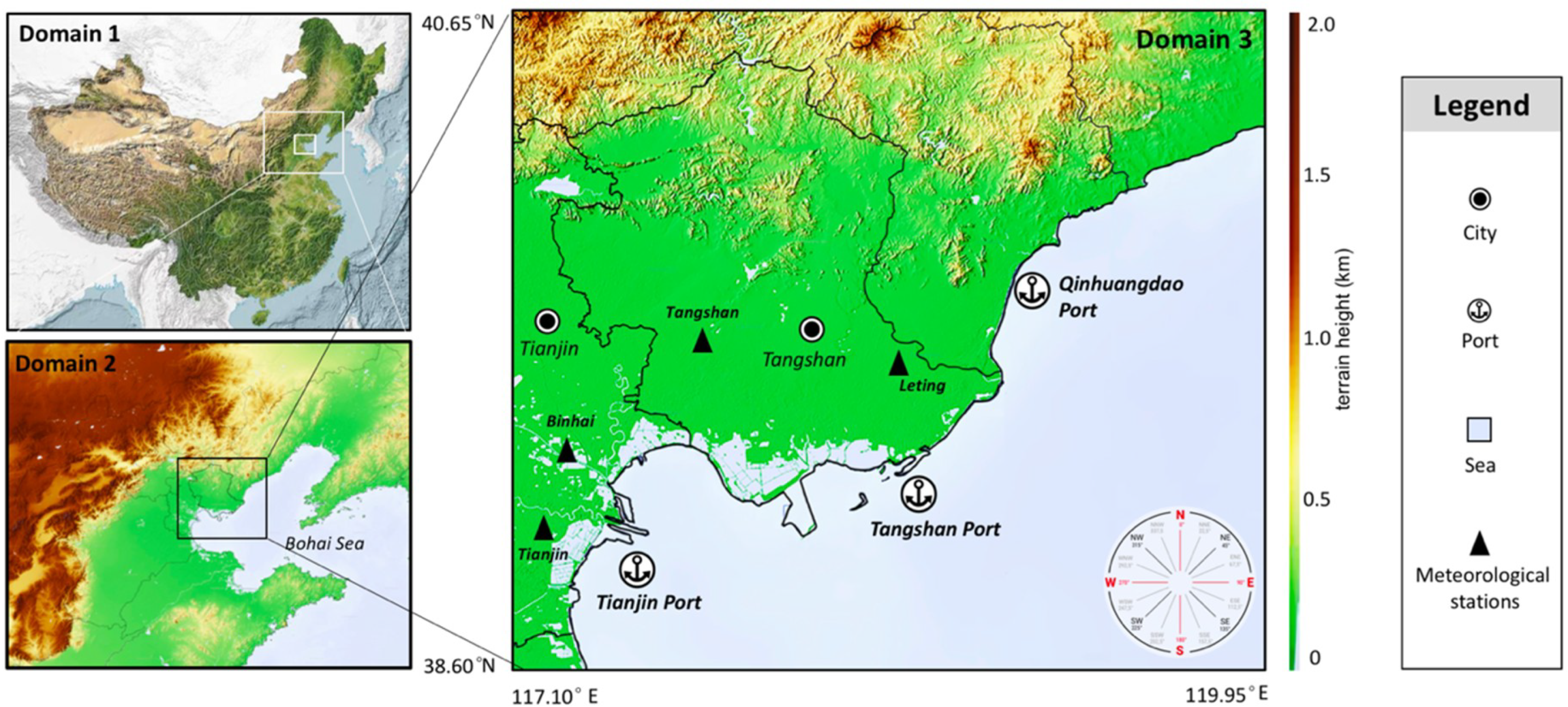
2.1. Study Area
2.2. Input Data and Model Configuration
2.2.1. Input Data
2.2.2. Model Configuration
2.3. Model Evaluation
- Cm = The model-estimated concentration at hour i
- Co = The observed concentration at hour i
- = The average model-estimated concentration of all hours
- = The average observed concentration of all hours
- N = The total numbers of hours for which the simulations are compared against observations
2.4. Identification of the Sea Breeze
3. Results and Discussion
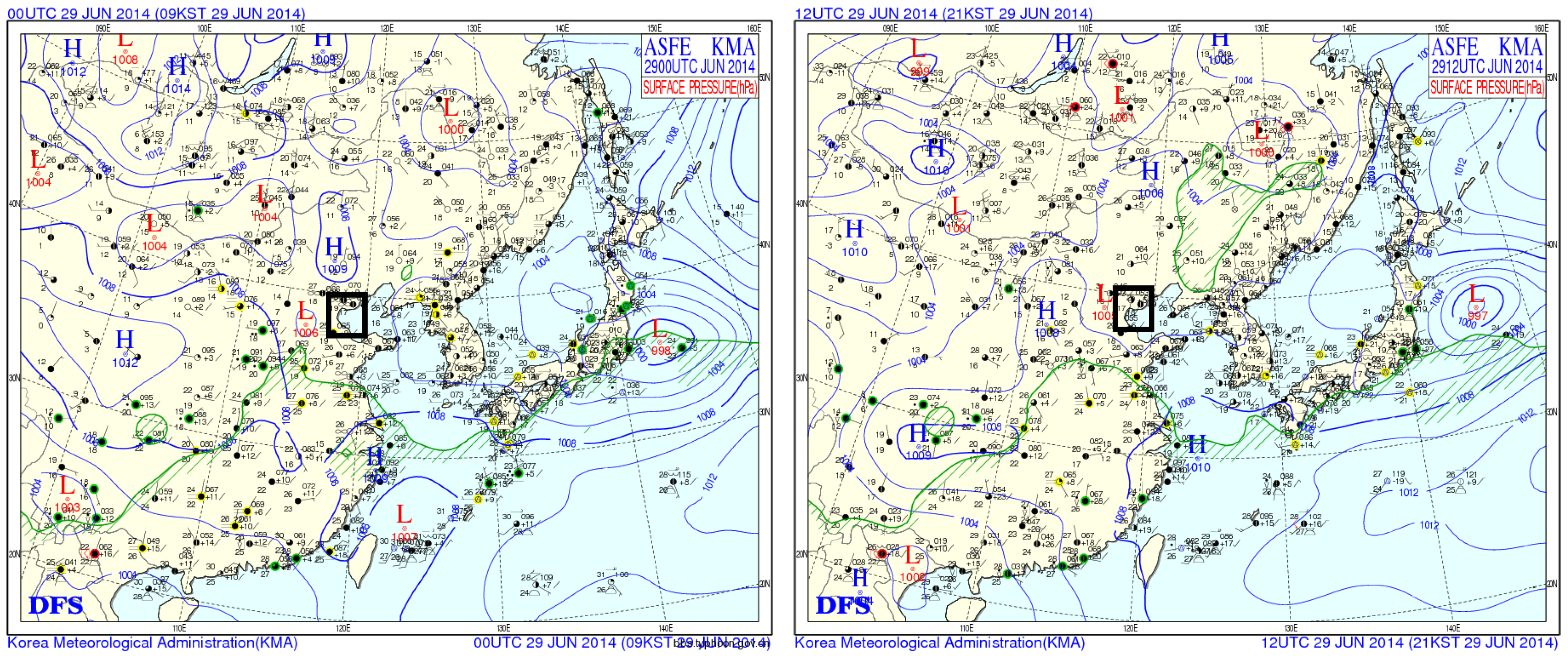
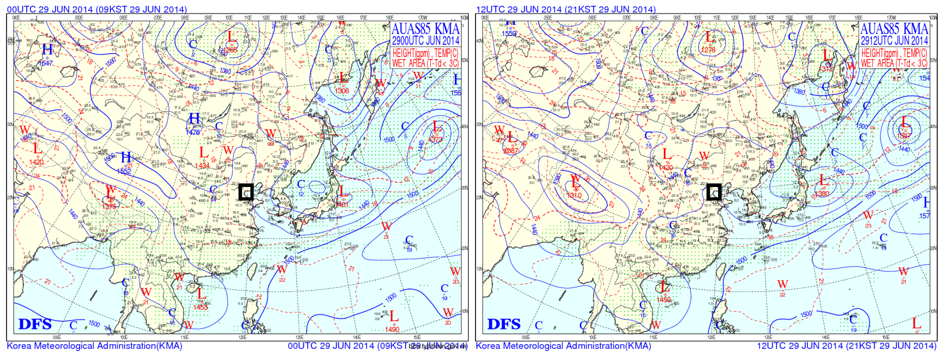
3.1. Synoptic Background
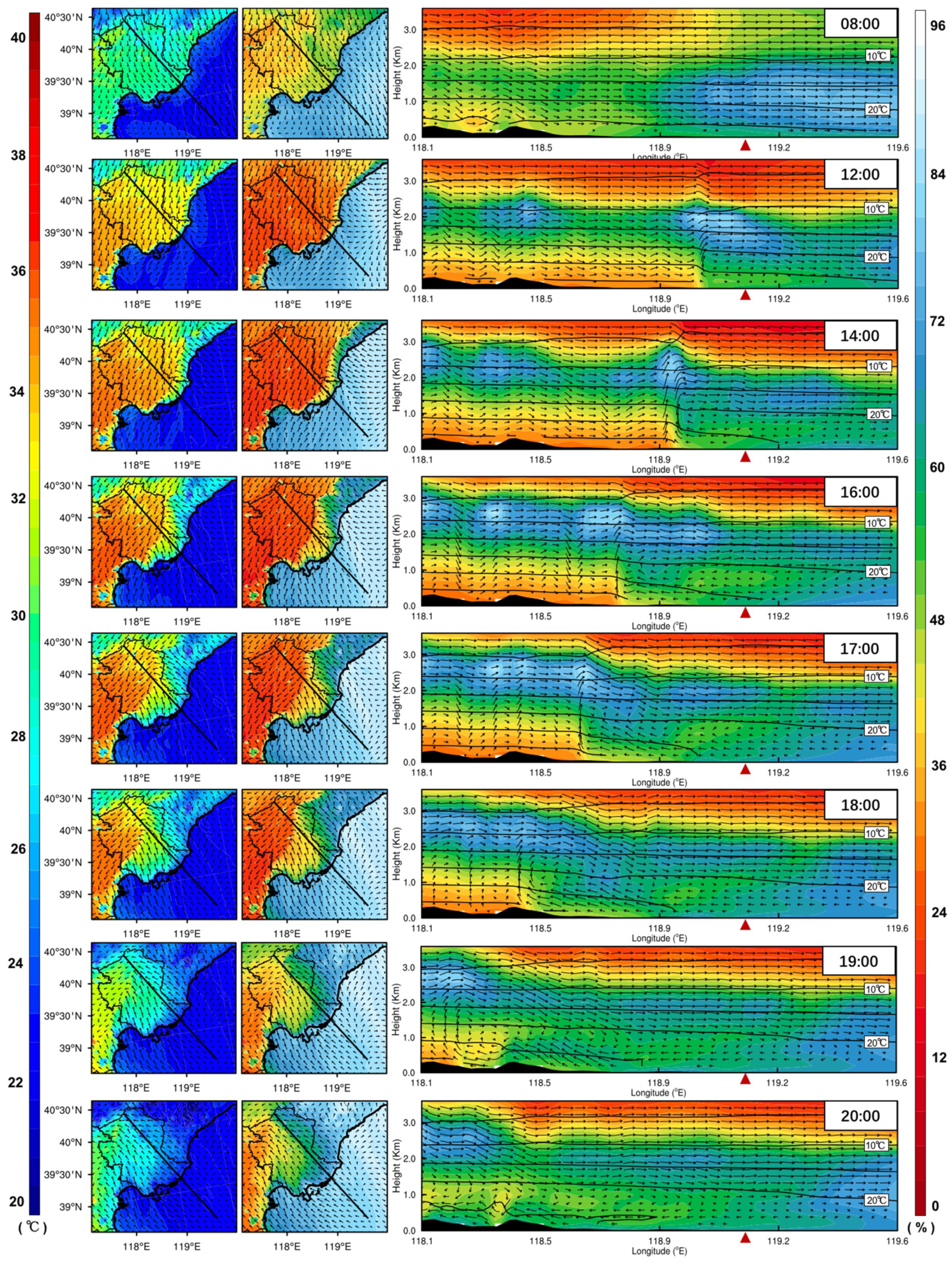
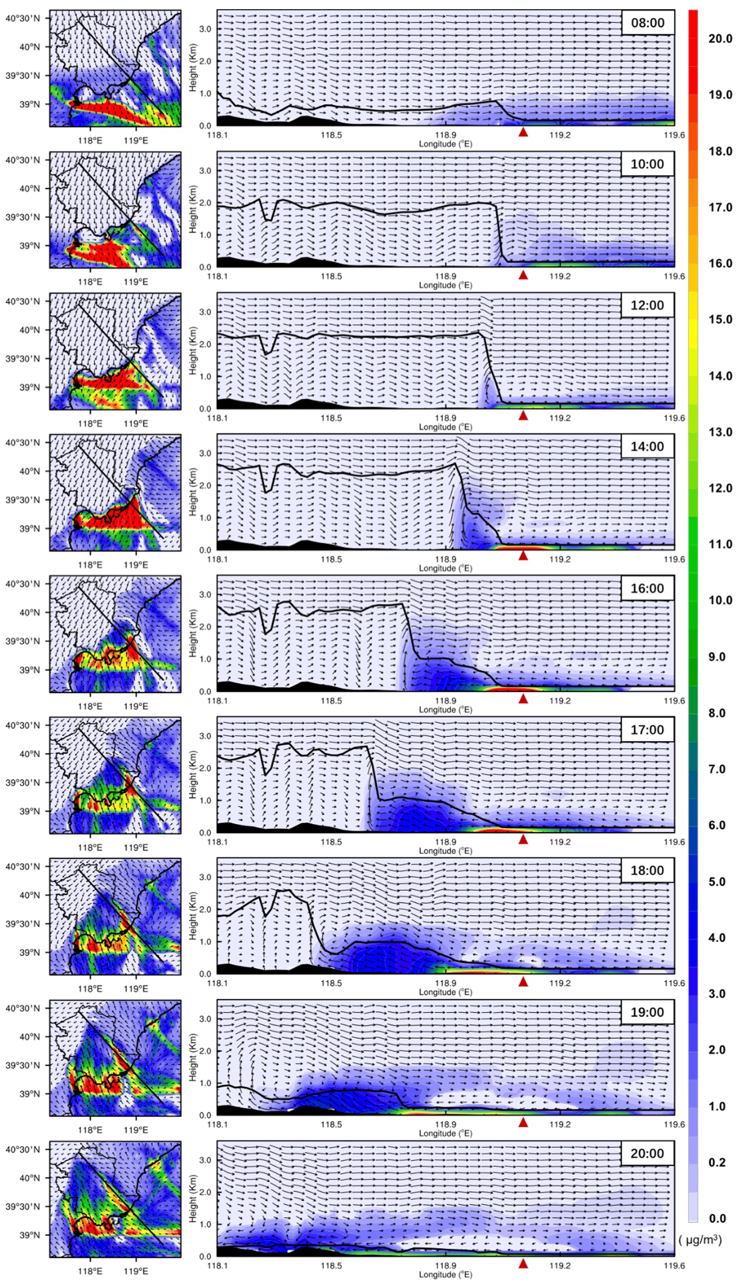
3.2. Development of the Sea Breeze Circulation
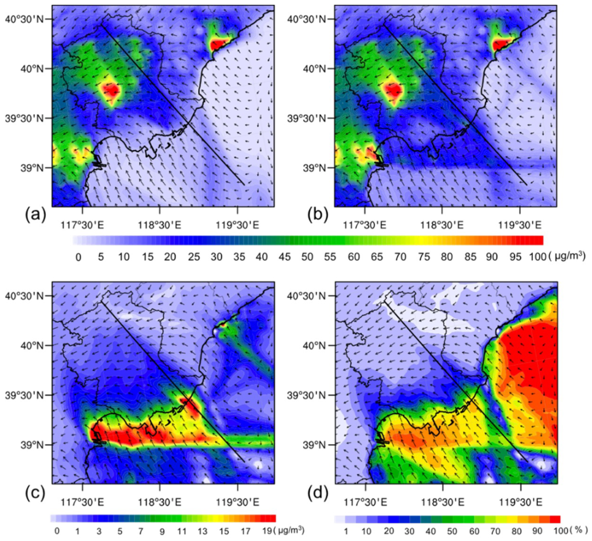
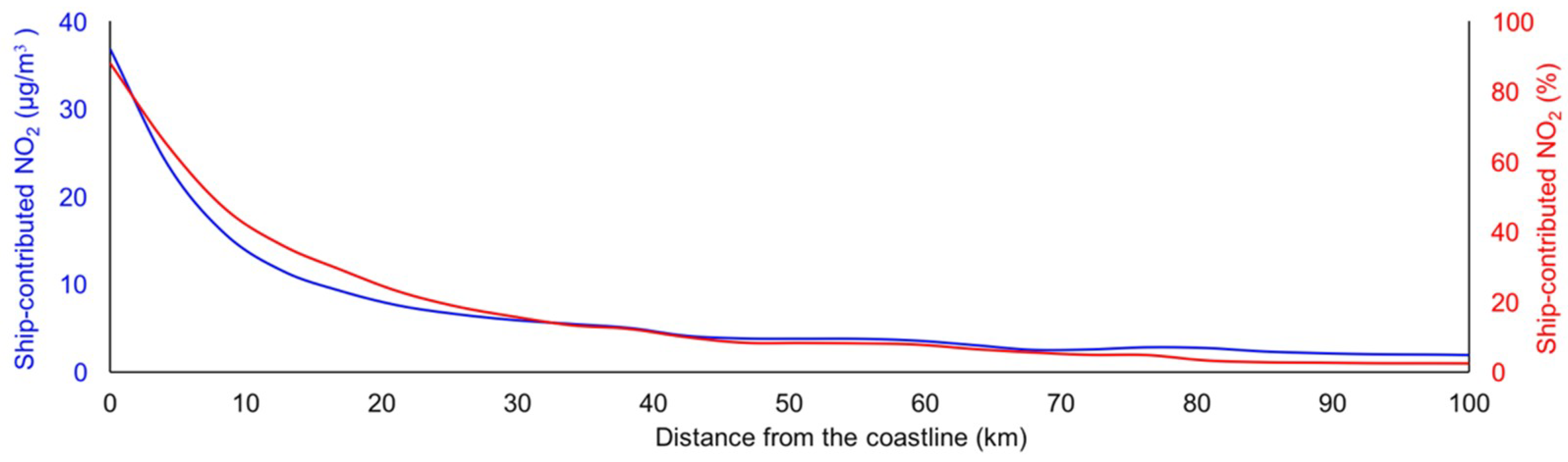
3.3. Impact of Sea Breeze on the Transport of Ship Emissions
4. Conclusions
Author Contributions
Funding
Acknowledgments
Conflicts of Interest
References
- Feng, J.; Zhang, Y.; Li, S.; Mao, J.; Patton, A.P.; Zhou, Y.; Ma, W.; Liu, C.; Kan, H.; Huang, C.; et al. The influence of spatiality on shipping emissions, air quality and potential human exposure in the Yangtze River Delta/Shanghai, China. Atmos. Chem. Phys. 2019, 19, 6167–6183. [Google Scholar] [CrossRef]
- Chen, D.; Tian, X.; Lang, J.; Zhou, Y.; Li, Y.; Guo, X.; Wang, W.; Liu, B. The impact of ship emissions on PM2.5 and the deposition of nitrogen and sulfur in Yangtze River Delta, China. Sci. Total Environ. 2019, 649, 1609–1619. [Google Scholar] [CrossRef]
- Murena, F.; Mocerino, L.; Quaranta, F.; Toscano, D. Impact on air quality of cruise ship emissions in Naples, Italy. Atmos. Environ. 2018, 187, 70–83. [Google Scholar] [CrossRef]
- Liu, H.; Meng, Z.H.; Shang, Y.; Lv, Z.F.; Jin, X.X.; Fu, M.L.; He, K.B. Shipping emission forecasts and cost-benefit analysis of China ports and key regions’ control. Environ. Pollut. 2018, 236, 49–59. [Google Scholar] [CrossRef]
- Liu, H.; Jin, X.; Wu, L.; Wang, X.; Fu, M.; Lv, Z.; Morawska, L.; Huang, F.; He, K. The impact of marine shipping and its DECA control on air quality in the Pearl River Delta, China. Sci. Total Environ. 2018, 625, 1476–1485. [Google Scholar] [CrossRef]
- Chen, D.; Zhao, N.; Lang, J.; Zhou, Y.; Wang, X.; Li, Y.; Zhao, Y.; Guo, X. Contribution of ship emissions to the concentration of PM2.5: A comprehensive study using AIS data and WRF/Chem model in Bohai Rim Region, China. Sci. Total Environ. 2018, 610–611, 1476–1486. [Google Scholar] [CrossRef]
- Zhang, Y.; Yang, X.; Brown, R.; Yang, L.P.; Morawska, L.; Ristovski, Z.; Fu, Q.Y.; Huang, C. Shipping emissions and their impacts on air quality in China. Sci. Total Environ. 2017, 581, 186–198. [Google Scholar] [CrossRef]
- Zhang, Y.; Gu, J.; Wang, W.; Peng, Y.; Wu, X.; Feng, X. Inland port vessel emissions inventory based on Ship Traffic Emission Assessment Model–Automatic Identification System. Adv. Mech. Eng. 2017, 9, 1687814017712878. [Google Scholar] [CrossRef]
- Liu, Z.; Lu, X.; Feng, J.; Fan, Q.; Zhang, Y.; Yang, X. Influence of Ship Emissions on Urban Air Quality: A Comprehensive Study Using Highly Time-Resolved Online Measurements and Numerical Simulation in Shanghai. Environ. Sci. Technol. 2017, 51, 202–211. [Google Scholar] [CrossRef]
- Jeong, J.-H.; Shon, Z.-H.; Kang, M.; Song, S.-K.; Kim, Y.-K.; Park, J.; Kim, H. Comparison of source apportionment of PM2.5 using receptor models in the main hub port city of East Asia: Busan. Atmos. Environ. 2017, 148, 115–127. [Google Scholar] [CrossRef]
- Becagli, S.; Anello, F.; Bommarito, C.; Cassola, F.; Calzolai, G.; Di Iorio, T.; di Sarra, A.; Gómez-Amo, J.-L.; Lucarelli, F.; Marconi, M.; et al. Constraining the ship contribution to the aerosol of the central Mediterranean. Atmos. Chem. Phys. 2017, 17, 2067–2084. [Google Scholar] [CrossRef]
- Yang, M.; Bell, T.G.; Hopkins, F.E.; Smyth, T.J. Attribution of atmospheric sulfur dioxide over the English Channel to dimethyl sulfide and changing ship emissions. Atmos. Chem. Phys. 2016, 16, 4771–4783. [Google Scholar] [CrossRef]
- Liu, H.; Fu, M.; Jin, X.; Shang, Y.; Shindell, D.; Faluvegi, G.; Shindell, C.; He, K. Health and climate impacts of ocean-going vessels in East Asia. Nat. Clim. Chang. 2016. [Google Scholar] [CrossRef]
- Fan, Q.; Zhang, Y.; Ma, W.; Ma, H.; Feng, J.; Yu, Q.; Yang, X.; Ng, S.K.W.; Fu, Q.; Chen, L. Spatial and seasonal dynamics of ship emissions over the Yangtze River Delta and East China Sea and their potential environmental influence. Environ. Sci. Technol. 2016, 50, 1322–1329. [Google Scholar] [CrossRef]
- Aksoyoglu, S.; Baltensperger, U.; Prévôt, A.S.H. Contribution of ship emissions to the concentration and deposition of air pollutants in Europe. Atmos. Chem. Phys. 2016, 16, 1895–1906. [Google Scholar] [CrossRef]
- Viana, M.; Fann, N.; Tobias, A.; Querol, X.; Rojas-Rueda, D.; Plaza, A.; Aynos, G.; Conde, J.A.; Fernandez, L.; Fernandez, C. Environmental and health benefits from designating the Marmara Sea and the Turkish Straits as an emission control area (ECA). Environ. Sci. Technol. 2015, 49, 3304–3313. [Google Scholar] [CrossRef]
- Zhao, M.; Zhang, Y.; Ma, W.; Fu, Q.; Yang, X.; Li, C.; Zhou, B.; Yu, Q.; Chen, L. Characteristics and ship traffic source identification of air pollutants in China’s largest port. Atmos. Environ. 2013, 64, 277–286. [Google Scholar] [CrossRef]
- Corbett, J.J. Global sulphur emissions inventories for ocean-going ships and their impact in global chemical transport models. J. Geophys. Res. Atmos. 1999, 104, 3457–3470. [Google Scholar] [CrossRef]
- Lv, Z.; Liu, H.; Ying, Q.; Fu, M.; Meng, Z.; Wang, Y.; Wei, W.; Gong, H.; He, K. Impacts of shipping emissions on PM2.5 pollution in China. Atmos. Chem. Phys. 2018, 18, 15811–15824. [Google Scholar] [CrossRef]
- Yau, P.S.; Lee, S.C.; Corbett, J.J.; Wang, C.; Cheng, Y.; Ho, K.F. Estimation of exhaust emission from ocean-going vessels in HongKong. Sci. Total Environ. 2012, 431, 299–306. [Google Scholar] [CrossRef]
- Dore, A.; Vieno, M.; Tang, Y.; Dragosits, U.; Dosio, A.; Weston, K.; Sutton, M. Modelling the atmospheric transport and deposition of sulphur and nitrogen over the United Kingdom and assessment of the influence of SO2 emissions from international shipping. Atmos. Environ. 2007, 41, 2355–2367. [Google Scholar] [CrossRef]
- Corbett, J.J.; Winebrake, J.J.; Green, E.H.; Kasibhatla, P.; Eyring, V.; Lauer, A. Mortality from Ship Emissions: A Global Assessment. Environ. Sci. Technol. 2007, 41, 8512–8518. [Google Scholar] [CrossRef]
- Masselink, G.; Pattiaratchi, C.B. The effect of sea breeze on beach morphology, surf zone hydrodynamics and sediment resuspension. Mar. Geol. 1998, 146, 115–135. [Google Scholar] [CrossRef]
- Huang, M.; Gao, Z.; Miao, S.; Xu, X. Characteristics of sea breezes over the Jiangsu coastal area, China. Int. J. Climatol. 2016, 36, 3908–3916. [Google Scholar] [CrossRef]
- Zhang, Z.Z.; Cao, C.X.; Song, Y.; Kang, L.; Cai, X.H. Statistical charactristics and numberical simulation of sea-land breezes in Hainan island. J. Trop. Meteorol. 2014, 20, 267–278. [Google Scholar]
- Rani, S.I.; Ramachandran, R.; Subrahamanyam, D.B.; Alappattu, D.P.; Kunhikrishnan, P.K. Characterization of sea/land breeze circulation along the west coast of Indian sub-continent during pre-monsoon season. Atmos. Res. 2010, 95, 367–378. [Google Scholar] [CrossRef]
- Eager, R.E.; Raman, S.; Wootten, A.; Westphal, D.L.; Reid, J.S.; Al Mandoos, A. A climatological study of the sea and land breezes in the Arabian Gulf region. J. Geophys. Res.-Atmos. 2008, 113. [Google Scholar] [CrossRef]
- Papanastasiou, D.K.; Melas, D. Climatology and impact on air quality of sea breeze in an urban coastal environment. Int. J. Climatol. 2009, 29, 305–315. [Google Scholar] [CrossRef]
- Yu, E.; Chen, B.; Bai, Y. Land and sea breezes in the weatern Bohai wan. Acta. Meteorol. 1987, 45, 379–381. [Google Scholar]
- Mavrakou, T.; Philippopoulos, K.; Deligiorgi, D. The impact of sea breeze under different synoptic patterns on air pollution within Athens basin. Sci. Total Environ. 2012, 433, 31–43. [Google Scholar] [CrossRef]
- Bouchlaghem, K.; Ben Mansour, F.; Elouragini, S. Impact of a sea breeze event on air pollution at the Eastern Tunisian Coast. Atmos. Res. 2007, 86, 162–172. [Google Scholar] [CrossRef]
- Miller, S.T.K.; Keim, B.D.; Talbot, R.W.; Mao, H. Sea breeze: Structure, forecasting, and impacts. Rev. Geophys. 2003, 41, 31. [Google Scholar] [CrossRef]
- Grossi, P.; Thunis, P.; Martilli, A.; Clappier, A. Effect of sea breeze on air pollution in the Greater Athens Area. Part II: Analysis of different emission scenarios. J. Appl. Meteorol. 2000, 39, 563–575. [Google Scholar] [CrossRef]
- Clappier, A.; Martilli, A.; Grossi, P.; Thunis, P.; Pasi, F.; Krueger, B.C.; Calpini, B.; Graziani, G.; van den Bergh, H. Effect of sea breeze on air pollution in the Greater Athens Area. Part I: Numerical simulations and field observations. J. Appl. Meteorol. 2000, 39, 546–562. [Google Scholar] [CrossRef]
- Kolev, I.; Parvanov, O.; Kaprielov, B.; Donev, E.; Ivanov, D. Lidar observations of sea-breeze and land-breeze aerosol structure on the Black Sea. J. Appl. Meteorol. 1998, 37, 982–995. [Google Scholar] [CrossRef]
- Camps, J.; Massons, J.; Soler, M.R. Numerical modelling of pollutant dispersion in sea breeze conditions. Ann. Geophys. Atmos. Hydrospheres Space Sci. 1996, 14, 665–677. [Google Scholar] [CrossRef]
- Rong Lu, R.P.T. Air pollutant transport in a coastal environment-II 3 dimensional simulations over los angeles basin. Atmos. Environ. 1995, 29, 1499–1518. [Google Scholar]
- Nester, K. Influence of sea breeze flows on air pollution over the attica peninsula. Atmos. Environ. 1995, 29, 3655–3670. [Google Scholar] [CrossRef]
- Physick, W.L.; Abbs, D.J. Flow and plume dispersion in a coastal valley. J. Appl. Meteorol. 1992, 31, 64–73. [Google Scholar] [CrossRef]
- Tsai, H.H.; Yuan, C.S.; Hung, C.H.; Lin, C.; Lin, Y.C. Influence of Sea-Land Breezes on the Tempospatial Distribution of Atmospheric Aerosols over Coastal Region. J. Air Waste Manag. Assoc. 2011, 61, 358–376. [Google Scholar] [CrossRef]
- Abbs, D.J.; Physick, W.L. Sea-breeze observations and modelling: A review. Aust. Meteorol. Mag. 1992, 41, 7–19. [Google Scholar]
- Levy, I.; Mahrer, Y.; Dayan, U. Coastal and synoptic recirculation affecting air pollutants dispersion: A numerical study. Atmos. Environ. 2009, 43, 1991–1999. [Google Scholar] [CrossRef]
- Boyouk, N.; Leon, J.F.; Delbarre, H.; Augustin, P.; Fourmentin, M. Impact of sea breeze on vertical structure of aerosol optical properties in Dunkerque, France. Atmos. Res. 2011, 101, 902–910. [Google Scholar] [CrossRef]
- Lin, W.S.; Wang, A.Y.; Wu, C.S.; Kun, F.S.; Ku, C.M. A case modeling of sea-land breeze in Macao and its neighborhood. Adv. Atmos. Sci. 2001, 18, 1231–1240. [Google Scholar]
- Prabha, T.; Venkatesan, R.; Mursch-Radlgruber, E.; Rengarajan, G.; Jayanthi, N. Thermal internal boundary layer characteristics at a tropical coastal site as observed by a mini-SODAR under varying synoptic conditions. J. Earth Syst. Sci. 2002, 111, 63–77. [Google Scholar] [CrossRef]
- Srinivas, C.V. Sensitivity of mesoscale simulations of land–sea breeze to boundary layer turbulence parameterization. Atmos. Environ. 2007, 41, 2534–2548. [Google Scholar] [CrossRef]
- Gangoiti, G.; Alonso, M.; Navazo, M.; Albizuri, A.; Perez-Landa, G.; Matabuena, M.; Valdenebro, V.; Maruri, M.; Garcia, J.; Millan, M.A. Regional transport of pollutants over the Bay of Biscay: Analysis of an ozone episode under a blocking anticyclone in west central Europe. Atmos. Environ. 2002, 36, 21349–21361. [Google Scholar] [CrossRef]
- Li, C.; Yuan, Z.; Ou, J.; Fan, X.; Ye, S.; Xiao, T.; Shi, Y.; Huang, Z.; Ng, S.K.; Zhong, Z.; et al. An AIS-based high-resolution ship emission inventory and its uncertainty in Pearl River Delta region, China. Sci. Total Environ. 2016, 573, 1–10. [Google Scholar] [CrossRef]
- Chen, D.; Zhao, Y.; Nelson, P.; Li, Y.; Wang, X.; Zhou, Y.; Lang, J.; Guo, X. Estimating ship emissions based on AIS data for port of Tianjin, China. Atmos. Environ. 2016, 145, 10–18. [Google Scholar] [CrossRef]
- Corbett, J.J.; Fischbeck, P.S.; Pandis, S.N. Global nitrogen and sulfur inventories for oceangoing ships. J. Geophys. Res.-Atmos. 1999, 104, 3457–3470. [Google Scholar] [CrossRef]
- Eyring, V.; Isaksen, I.; Berntsen, T.; Collins, W.; Corbett, J.J.; Endresen, O.; Grainger, R.G.; Moldanova, J.; Schlager, H.; Stevenson, D.S. Transport impacts on atmosphere and climate: Shipping. Atmos. Environ. 2010, 44, 4735–4771. [Google Scholar] [CrossRef]
- Eyring, V.; Kohler, H.W.; van Aardenne, J.; Lauer, A. Emissions from international shipping: 1. The last 50 years. J. Geophys. Res. Atmos. 2005, 110, 12. [Google Scholar] [CrossRef]
- Chen, D.; Zhang, Y.; Lang, J.; Ying, Z.; Li, Y.; Guo, X.; Wang, W.; Liu, B. Evaluation of different control measures in 2014 to mitigate the impact of ship emissions on air quality in the Pearl River Delta, China. Atmos. Environ. 2019, 216, 116911. [Google Scholar] [CrossRef]
- Tao, J.; Zhang, L.; Cao, J.; Zhong, L.; Chen, D.; Yang, Y.; Chen, D.; Chen, L.; Zhang, Z.; Wu, Y.; et al. Source apportionment of PM2.5 at urban and suburban areas of the Pearl River Delta region, south China - With emphasis on ship emissions. Sci. Total Environ. 2017, 574, 1559–1570. [Google Scholar] [CrossRef]
- Chen, D.; Wang, X.; Nelson, P.; Li, Y.; Zhao, N.; Zhao, Y.; Lang, J.; Zhou, Y.; Guo, X. Ship emission inventory and its impact on the PM2.5 air pollution in Qingdao Port, North China. Atmos. Environ. 2017, 166, 351–361. [Google Scholar] [CrossRef]
- Contini, D.; Gambaro, A.; Donateo, A.; Cescon, P.; Cesari, D.; Merico, E.; Belosi, F.; Citron, M. Inter-annual trend of the primary contribution of ship emissions to PM2.5 concentrations in Venice (Italy): Efficiency of emissions mitigation strategies. Atmos. Environ. 2015, 102, 183–190. [Google Scholar] [CrossRef]
- Tao, L.; Fairley, D.; Kleeman, M.J.; Harley, R.A. Effects of switching to lower sulfur marine fuel oil on air quality in the San Francisco Bay area. Environ. Sci. Technol. 2013, 47, 10171–10178. [Google Scholar] [CrossRef]
- MOT of China. Available online: http://xxgk.mot.gov.cn/jigou/zhghs/201905/t20190513_3198921.html (accessed on 20 October 2019).
- Grell, G.; Peckham, S.; Schmitz, R.; McKeen, S.; Frost, G.; Skamarock, W.; Eder, B. Fully coupled “online” Chemistry within the WRF model. Atmos. Environ. 2005, 39, 6957–6975. [Google Scholar] [CrossRef]
- Chen, D.; Wang, X.; Li, Y.; Lang, J.; Zhou, Y.; Guo, X.; Zhao, Y. High-spatiotemporal-resolution ship emission inventory of China based on AIS data in 2014. Sci. Total Environ. 2017, 609, 776–787. [Google Scholar] [CrossRef]
- Liu, F.; Zhang, Q.; Tong, D.; Zheng, B.; Li, M.; Huo, H.; He, K. High-resolution inventory of technologies, activities, and emissions of coal-red power plants in China from 1990 to 2010. Atmos. Chem. Phys. 2015, 15, 13299–13317. [Google Scholar] [CrossRef]
- Zheng, B.; Huo, H.; Zhang, Q.; Yao, Z.; Wang, X.; Yang, X.; Liu, H.; He, K. High-resolution mapping of vehicle emissions in China in 2008. Atmos. Chem. Phys. 2014, 14, 9787–9805. [Google Scholar] [CrossRef]
- Li, M.; Zhang, Q.; Streets, D.; He, K.; Cheng, Y.; Emmons, L.; Huo, H.; Kang, S.; Lu, Z.; Shao, M.; et al. Mapping Asian anthropogenic emissions of non-methane volatile organic compounds to multiple Chemical me-chanisms. Atmos. Chem. Phys. 2014, 14, 5617–5638. [Google Scholar] [CrossRef]
- Zhang, Q.; Streets, D.; Carmichael, G.; He, K.; Huo, H.; Kannari, A.; Klimont, Z.; Park, I.; Reddy, S.; Fu, J.; et al. Asian emissions in 2006 for the NASA INTEX-B mission. Atmos. Chem. Phys. 2009, 9, 5131–5153. [Google Scholar] [CrossRef]
- MEIC. Available online: http://www/. meicmodel.org/ (accessed on 20 October 2019).
- Zhou, Y.; Xing, X.; Lang, J.; Chen, D.; Cheng, S.; Wei, L.; Wei, X.; Liu, C. A comprehensive biomass burning emission inventory with high spatial and temporal resolution in China. Atmos. Chem. Phys. Discuss. 2016, 1–43. [Google Scholar] [CrossRef]
- NCEP. Available online: https://doi.org/10.5065/D6M043C6 (accessed on 1 September 2019).
- Stockwell, W.; Middleton, P.; Chang, J.; Tang, X. The second generation regional acid deposition model Chemical mechanism for regional air quality modeling. J. Geophys. Res. Atmos. 1990, 95, 16343–16367. [Google Scholar] [CrossRef]
- Schell, B.; Ackermann, I.; Hass, H.; Binkowski, F.; Ebel, A. Modeling the formation of secondary organic aerosol within a comprehensive air quality model system. J. Geophys. Res. Atmos. 2001, 106, 28275–28293. [Google Scholar] [CrossRef]
- Ackermann, I.; Hass, H.; Memmesheimer, M.; Ebel, A.; Binkowski, F.; Shankar, U. Modal aerosol dynamics model for Europe: Development and first applications. Atmos. Environ. 1998, 32, 2981–2999. [Google Scholar] [CrossRef]
- Hong, S.; Noh, Y.; Dudhia, J. A new vertical diffusion package with an explicit treatment of entrainment processes. Mon. Weather Rev. 2006, 134, 2318–2341. [Google Scholar] [CrossRef]
- Fels, S.; Schwarzkopf, M. An efficient, accurate algorithm for calculating CO2 15 μm band cooling rates. J. Geophys. Res. Atmos. 1981, 86, 1205–1232. [Google Scholar] [CrossRef]
- Chou, M.; Suarez, M. A solar radiation parameterization for atmospheric studies. NASA Tech. Memo. 1999, 15, 40. [Google Scholar]
- Lin, Y.; Farley, R.; Orville, H. Bulk Parameterization of the snow field in a cloud model. J. Clim. Appl. Meteorol. 1983, 22, 1065–1092. [Google Scholar] [CrossRef]
- Ek, M.; Mitchell, K.; Lin, Y.; Rogers, B.; Grunmann, P.; Koren, V.; Gayno, G.; Tarpley, J. Implementation of NOAH land surface model advances in the National Centers for Environmental Prediction operational mesoscale Eta model. J. Geophys. Res. 2003, 108, 8851. [Google Scholar] [CrossRef]
- Xu, Z.; Liu, M.; Song, Y.; Zhang, M.; Wang, S.; Xu, T.; Zhang, L.; Wang, T.; Yan, C.; Zhou, T.; et al. High efficiency of livestock ammonia emission controls on alleviating particulate nitrate during a severe winter haze episode in northern China. Atmos. Chem. Phys. 2019, 19, 5605–5613. [Google Scholar]
- Liu, M.; Huang, X.; Song, Y.; Xu, T.; Wang, S.; Wu, Z.; Hu, M.; Zhang, L.; Zhang, Q.; Pan, Y.; et al. Rapid SO2 emission reductions significantly increase tropospheric ammonia concentrations over the North China Plain. Atmos. Chem. Phys. 2018, 18, 17933–17943. [Google Scholar] [CrossRef]
- Liu, M.; Huang, X.; Song, Y.; Tang, J.; Cao, J.; Zhang, X.; Zhang, Q.; Wang, S.; Xu, T.; Kang, L.; et al. Complex Impacts of Ammonia Emission Control in China: Improved Haze Pollution, Reduced Nitrogen Deposition, but Worsened Acid Rain. Proc. Natl. Acad. Sci. USA 2018, 116, 7760–7765. [Google Scholar] [CrossRef]
- Yao, H.; Song, Y.; Liu, M.; Archer-Nicholls, S.; Lowe, D.; McFiggans, G.; Xu, T.; Du, P.; Li, J.; Wu, Y.; et al. Direct radiative effect of carbonaceous aerosols from crop residue burning during the summer harvest season in East China. Atmos. Chem. Phys. 2017, 17, 5205–5520. [Google Scholar] [CrossRef]
- Liu, L.; Huang, X.; Ding, A.; Fu, C. Dust-induced radiative feedbacks in north China: A dust storm episode modeling study using WRF-Chem. Atmos. Environ. 2016, 129, 43–54. [Google Scholar] [CrossRef]
- Gao, M.; Carmichael, G.R.; Saide, P.E.; Lu, Z.; Yu, M.; Streets, D.G.; Wang, Z. Response of winter fine particulate matter concentrations to emission and meteorology changes in North China. Atmos. Chem. Phys. 2016, 16, 11837–11851. [Google Scholar] [CrossRef]
- NCEI. Available online: https://gis.ncdc.noaa.gov/maps/ncei/cdo/hourly (accessed on 20 July 2019).
- Kwok, R.H.; Fung, J.C.; Lau, A.K.; Fu, J.S. Numerical study on seasonal variations of gaseous pollutants and particulate matters in Hong Kong and Pearl River Delta Region. J. Geophys. Rse. Atmos. 2010, 115, D16308. [Google Scholar] [CrossRef]
- Zhang, Y.; Liu, P.; Pun, B.; Seigneur, C. A comprehensive performance evaluation of MM5-CMAQ for the Summer 1999 Southern Oxidants Study episode Part I: Evaluation protocols, databases, and meteorological predictions. Atmos. Environ. 2006, 40, 4825–4838. [Google Scholar] [CrossRef]
- Boylan, J.; Russel, A. PM and light extinction model performance metrics, goals, and criteria for three-dimensional air quality models. Atmos. Environ. 2006, 40, 4946–4959. [Google Scholar] [CrossRef]
- Liao, J.; Wang, T.; Jiang, Z.; Zhuang, B.; Xie, M.; Yin, C.; Wang, X.; Zhu, J.; Fu, Y.; Zhang, Y. WRF/Chem modeling of the impacts of urban expansion on regional climate and air pollutants in Yangtze River Delta, China. Atmos. Environ. 2015, 106, 204–214. [Google Scholar] [CrossRef]
- Zhang, Y.; Wen, X.Y.; Jang, C.J. Simulating Chemistry–aerosol–clould–radiation–climate feedbacks over the continental U.S. using the online-coupled Weather Research Forecasting Model with Chemistry (WRF/Chem). Atmos. Environ. 2010, 44, 3568–3582. [Google Scholar] [CrossRef]
- Borne, K.; Chen, D.; Nunez, M. A method for finding sea breeze days under stable synoptic conditions and its application to the swedish west coast. Int. J. Climatol. 1998, 18, 901–904. [Google Scholar] [CrossRef]
- Furberg, M.; Steyn, D.G.; Baldi, M. The climatology of sea breezes on Sardinia. Int. J. Climatol. 2002, 22, 917–932. [Google Scholar] [CrossRef]
- Azorin-Molina, C.; Tijm, S.; Chen, D. Development of selection algorithms and databases for sea breeze studies. Theor. Appl. Climatol. 2011, 106, 531–546. [Google Scholar] [CrossRef]
- Miao, J.F.; Chen, D.; Wyser, K.; Borne, K.; Lindgren, J.; Strandevall, M.K.S.; Thorsson, S.; Achberger, C.; Almkvist, E. Evaluation of MM5 mesoscale model at local scale for air quality applications over the Swedish west coast: Influence of PBL and LSM parameterizations. Meteorol. Atmos. Phys. 2008, 99, 77–103. [Google Scholar] [CrossRef]
- Arritt, R. Effects of the Large-Scale flow on Characteristic features of the sea breeze. J. Appl. Meteorol. 1992, 32, 116–125. [Google Scholar] [CrossRef]


| Sectors | Emission (tons/month) | Contribution of the emission |
|---|---|---|
| Transportation | 12979 | 15.56 % |
| Industry | 37330 | 44.75 % |
| Residential | 715 | 0.86 % |
| Power | 24836 | 29.77 % |
| Biomass burning | 535 | 0.64 % |
| Total non-ship emissions | 76395 | 91.58 % |
| Ship emissions | 7018 | 8.42 % |
| Total emissions | 83413 | 100% |
| Chemical and Physics Options | Schemes | Reference | |
|---|---|---|---|
| Chemical Schemes | Gas-phase | The Regional Acid Deposition Model version 2 (RMD2) | Stockwell et al. [68] |
| Aerosol | The Modal Aerosol Dynamics Model for Europe (MADE/SORGAM) | Ackermann et al. [69]; Schell et al. [70] | |
| Physics Schemes | Planetary Boundary layer | Yonsei University (YSU) | Hong et al. [71] |
| Longwave Radiation | Eta Geophysical Fluid Dynamics Laboratory (GFDL) | Fels and Schwarzkopf [72] | |
| Shortwave Radiation | Goddard | Chou and Suarez [73] | |
| Microphysics | Purdue Lin | Lin et al. [74] | |
| Land Surface Model | Noah | Ek et al. [75] | |
| Sites | Vars | MBa | MAEb | NMBc (%) | NMEd (%) | Re |
|---|---|---|---|---|---|---|
| Tianjin | T2 | 0.82 | 1.96 | 6.20 | 6.66 | 0.91 |
| RH2 | −15.18 | 15.18 | −22.63 | 32.63 | 0.82 | |
| WS10 | 0.38 | 0.66 | 15.83 | 27.63 | 0.82 | |
| WD10 | 8.80 | 25.78 | 9.82 | 16.88 | 0.75 | |
| Binhai | T2 | −0.23 | 1.73 | −0.77 | 5.76 | 0.92 |
| RH2 | −1.05 | 8.59 | −2.63 | 21.61 | 0.85 | |
| WS10 | 0.32 | 0.65 | 11.22 | 22.62 | 0.80 | |
| WD10 | 6.59 | 24.82 | 22.86 | 31.81 | 0.76 | |
| Tangshan | T2 | 1.01 | 1.43 | 3.60 | 5.10 | 0.92 |
| RH2 | −12.06 | 12.06 | −22.45 | 22.45 | 0.84 | |
| WS10 | 0.45 | 0.76 | 12.12 | 34.78 | 0.79 | |
| WD10 | 5.33 | 26.62 | 18.13 | 29.13 | 0.72 | |
| Leting | T2 | −0.06 | 2.38 | −0.22 | 9.31 | 0.91 |
| RH2 | −6.53 | 20.73 | −11.16 | 38.61 | 0.83 | |
| WS10 | 0.50 | 1.05 | 18.97 | 37.00 | 0.82 | |
| WD10 | 7.92 | 30.02 | 17.91 | 33.74 | 0.79 |
| Sites | NMBa (%) | NMEb (%) | MFBc (%) | MFEd (%) | Re |
|---|---|---|---|---|---|
| Tianjin | −12.27 | 19.91 | −13.07 | 17.98 | 0.95 |
| Tangshan | −2.32 | 16.61 | −6.30 | 13.54 | 0.90 |
© 2019 by the authors. Licensee MDPI, Basel, Switzerland. This article is an open access article distributed under the terms and conditions of the Creative Commons Attribution (CC BY) license (http://creativecommons.org/licenses/by/4.0/).
Share and Cite
Shang, F.; Chen, D.; Guo, X.; Lang, J.; Zhou, Y.; Li, Y.; Fu, X. Impact of Sea Breeze Circulation on the Transport of Ship Emissions in Tangshan Port, China. Atmosphere 2019, 10, 723. https://doi.org/10.3390/atmos10110723
Shang F, Chen D, Guo X, Lang J, Zhou Y, Li Y, Fu X. Impact of Sea Breeze Circulation on the Transport of Ship Emissions in Tangshan Port, China. Atmosphere. 2019; 10(11):723. https://doi.org/10.3390/atmos10110723
Chicago/Turabian StyleShang, Fang, Dongsheng Chen, Xiurui Guo, Jianlei Lang, Ying Zhou, Yue Li, and Xinyi Fu. 2019. "Impact of Sea Breeze Circulation on the Transport of Ship Emissions in Tangshan Port, China" Atmosphere 10, no. 11: 723. https://doi.org/10.3390/atmos10110723
APA StyleShang, F., Chen, D., Guo, X., Lang, J., Zhou, Y., Li, Y., & Fu, X. (2019). Impact of Sea Breeze Circulation on the Transport of Ship Emissions in Tangshan Port, China. Atmosphere, 10(11), 723. https://doi.org/10.3390/atmos10110723