Article

Geographical Imputation of Missing Poaceae Pollen Data via Convolutional Neural Networks

by
Ricardo Navares
and
José Luis Aznarte
*
Department of Artificial Intelligence, UNED, Juan del Rosal, 16, 28040 Madrid, Spain
*
Author to whom correspondence should be addressed.
Atmosphere 2019, 10(11), 717; https://doi.org/10.3390/atmos10110717
Submission received: 4 October 2019 / Revised: 13 November 2019 / Accepted: 14 November 2019 / Published: 16 November 2019
(This article belongs to the Special Issue GIS Applications for Airborne Pollen Monitoring and Prediction)

Abstract

:
Airborne pollen monitoring datasets sometimes exhibit gaps, even very long, either because of maintenance or because of a lack of expert personnel. Despite the numerous imputation techniques available, not all of them effectively include the spatial relations of the data since the assumption of missing-at-random is made. However, there are several techniques in geostatistics that overcome this limitation such as the inverse distance weighting and Gaussian processes or kriging. In this paper, a new method is proposed that utilizes convolutional neural networks. This method not only shows a competitive advantage in terms of accuracy when compared to the aforementioned techniques by improving the error by 5% on average, but also reduces execution training times by 90% when compared to a Gaussian process. To show the advantages of the proposal, 10%, 20%, and 30% of the data points are removed in the time series of a Poaceae pollen observation station in the region of Madrid, and the airborne concentrations from the remaining available stations in the network are used to impute the data removed. Even though the improvements in terms of accuracy are not significantly large, even if consistent, the gain in computational time and the flexibility of the proposed convolutional neural network allow field experts to adapt and extend the solution, for instance including meteorological variables, with the potential decrease of the errors reported in this paper.

1. Introduction

The clinical relevance of Poaceae pollen has been increasing as the number of allergy cases continues to grow [1], which is expected to double in the next 40 years [2]. Limiting exposure to airborne pollen plays a key role in the prevention of symptoms. The prediction of future pollen concentrations is thus crucial, not only for patients, but also for clinical institutions, in order to arrange resources before the influx of pollen related allergy cases.
Observation based models employ different methods to relate records of air concentrations to one or more variables that can be measured or predicted. Examples include regression models [3,4], time series models [5], and process based phenological models [6]. In the last decade, machine learning techniques have been gaining importance due to the success of their applications [4,7,8,9,10,11,12]. However, these techniques require a significant amount of data, and when dealing with pollen time series, where high concentrations are especially harmful when they are over 25 grains/m 3 [1], the data are incomplete during the full year (Figure 1). Even though there have been advances in automatic pollen monitoring [13], the European volumetric spore trap network is mostly operated manually. Furthermore, defects and maintenance imply that pollen observation networks are highly sensitive to missing data points.
Despite the numerous techniques available for missing data imputation, most of the literature focuses on the conditions under which they lead to unbiased estimates, conditions that do not often hold. There is no consensus about the exact proportion of missing data for which it is considered unacceptable to use such techniques. For instance, Schafer [14] asserted that less than 5% is inconsequential, while Bennett [15] claimed that statistical analysis is likely to be biased over 10%. In this proposal, we use 10%, 20%, and 30% of missing data, which are greater amounts than asserted by previous literature. Moreover, many techniques do not take into consideration the spatial relations of the data. Geographical imputation overcomes this problem by estimating missing data points with approximate locations derived from associated data. Among the techniques available, inverse distance weighting [16] and kriging or Gaussian process regression [17] are two of the most popular among field experts.
However, in the last few decades, artificial intelligence methods have been gaining attention due to their competitive advantage in solving real-world problems [18]. In particular, convolutional neural networks (CNNs) [19] have been proven very effective in areas such as computer vision [20] and natural language processing [21]. The main difference from traditional neural networks lies in using the convolution operation [22] applied to filters, which allows exploiting the strong, spatial correlation present in the data.
Even though there is extensive literature about computational intelligence techniques applied to pollen time series, such as random forests [7,12,23,24], artificial neural networks [9,10], and deep neural architectures [25], very few works have applied convolutional neural networks to time series. Nonetheless, CNNs have been extensively used in identifying and classifying pollen grains [26,27].
The objective of this paper is to extend the application of CNNs and increase the awareness of their advantage and potential. In order to do so, we propose a network architecture that will be compared to the aforementioned traditional spatial imputation techniques. By artificially producing missing data points in the time series of one of the observation stations in the region of Madrid, the study estimates such points from the available observations from the surrounding stations.

2. Materials and Methods

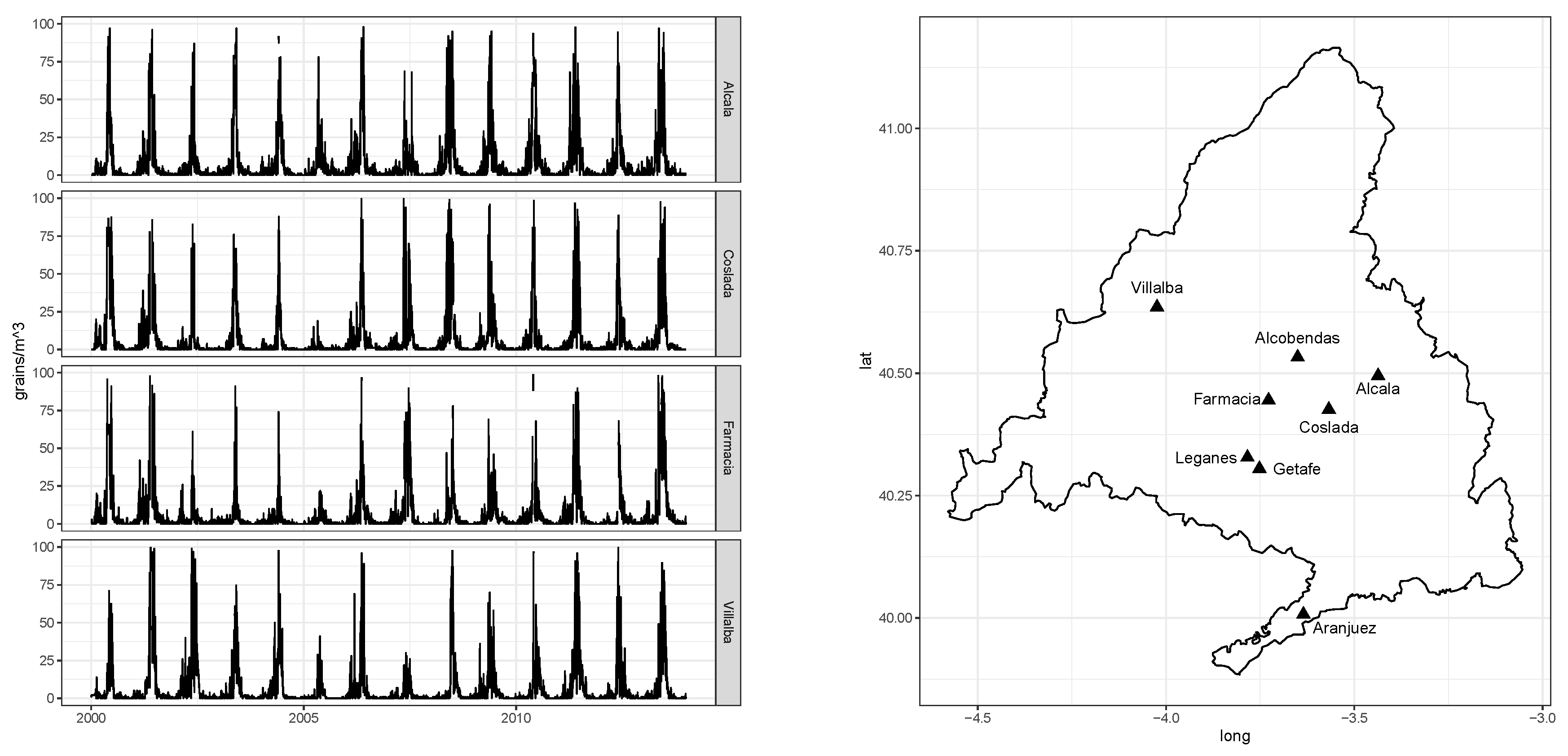
2.1. Data Description
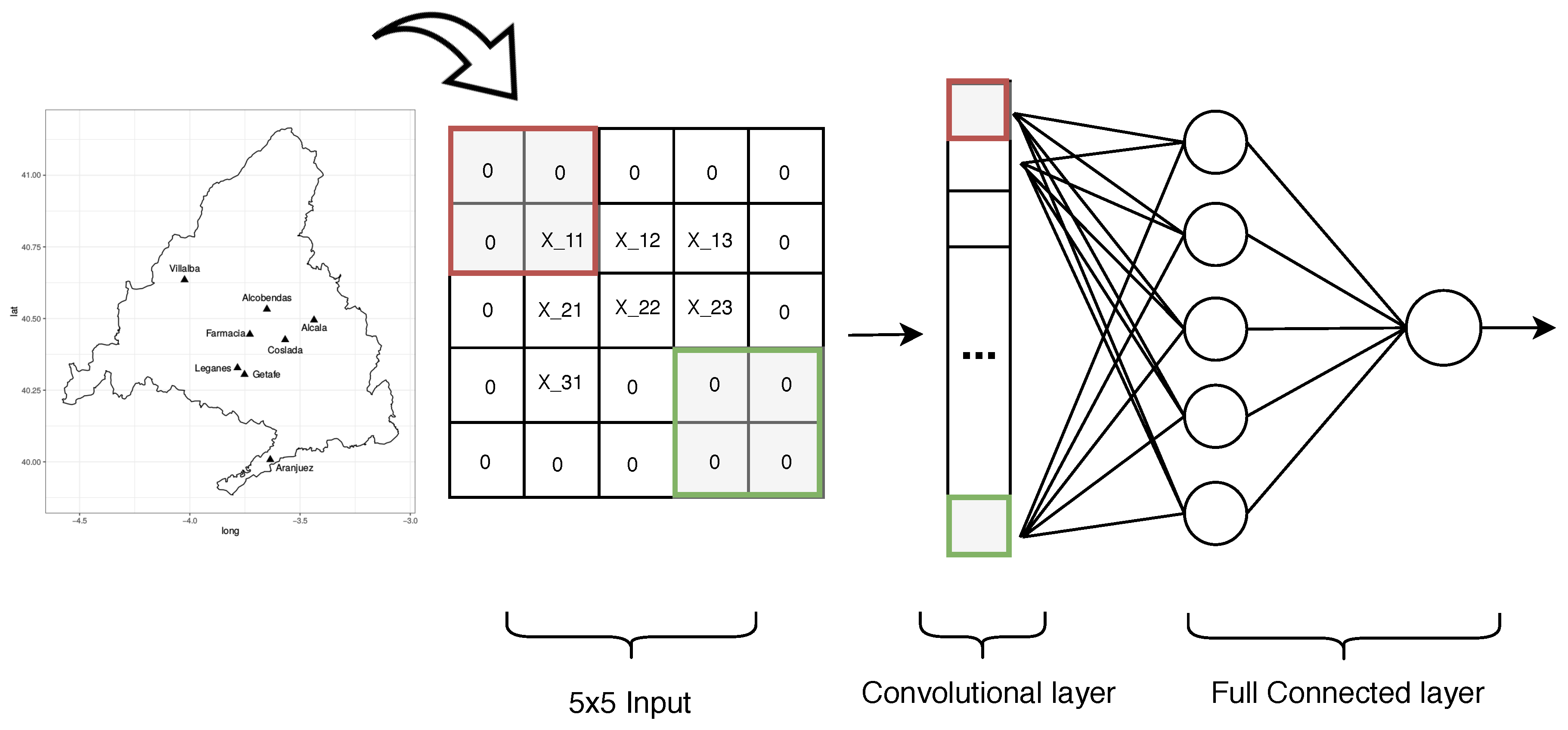
Poaceae pollen observations were provided daily in grains per cubic meter registered at eight locations in or around the city of Madrid: Alcalá de Henares, Alcobendas, Aranjuez, Complutense University of Madrid (Pharmacy Faculty), Coslada, Getafe, Leganés, and Villalba. Series for these locations are shown in Figure 1. Pollen counts followed the standard methodology of the Spanish Aerobiological Network [28] and were provided by Red Palinológica de la Comunidad de Madrid. Observations were available for 14 years starting from 1 January 2000 to 31 December 2013.
The region of Madrid has particular geographical characteristics (Figure 1). The observation station in Aranjuez is at the lowest elevation (495 m above sea level) and has a yearly average temperature above 14 C with a yearly average rainfall below 400 mm. On the other hand, Villalba is located 903 m above sea level with a yearly average temperature of 10–11 C and a yearly average precipitation of 1250–1500 mm. The remaining locations are in metropolitan areas between 594 and 668 m above sea level with yearly average temperatures above 15.2 C and precipitation around 440 mm.

2.2. Methodology

Inverse distance weighted (IDW) interpolation is based on the principle that nearer observations are more related than distant ones [29]. Consequently, pollen counts measured closer to the location of the station for which we want to estimate the pollen counts will have more influence than those that are distant. This influence is represented by the distance, and the estimation y j ^ is calculated as the weighted sum of the measured pollen counts at the observation stations x i :
y j ^ = i = 1 n x i d i j p i = 1 n 1 d i j p ,
where n is the number of observation stations, d i j is the distance between the observation station i and the observation station j where we want to estimate the pollen count, and p is the power function, which is set to 2 as the default value.
While in IDW, the power function defines how fast the influence (weight) of an observed pollen count measure decreases based on distance, a Gaussian process or kriging [17] creates a model of spatial correlation that provides the proper weights by relying on the covariance matrix to control the values that are close together in the input space to generate values that are similar. A Gaussian process (GP) assumes that the probability p ( f ( x 1 ) , , f ( x n ) ) is jointly Gaussian, x i being the set of observed points, with mean μ and covariance given by i j = k ( x i , x j ) , where k is the kernel function [30]. The underlying idea is that having the joint probability of the variables, it is possible to get the conditional probability of one of the variables given the others [31].
Based on their success in other fields, experts have started to use convolutional neural networks for time series analysis [32]. CNNs differ from feedforward neural networks mainly by the existence of convolutional layers, which are hidden layers that utilize the power of the mathematical operation of convolution to transform the inputs. Convolution allows for the encoding of the local properties of the input in such a way that the information propagates in a more efficient manner. CNN filters, obtained by the convolution of inputs and weights, are local in input space and are thus able to exploit the strong, spatial correlation present in the time series. That means that they work well in identifying simple patterns within local regions of the data (subset of features), which then will be used by subsequent layers to form more complex patterns.
In order to compare the results with similar research studies, the common scoring rule of the root mean squared error (RMSE) will be used to measure the average magnitude of the error.

2.3. Experimental Design
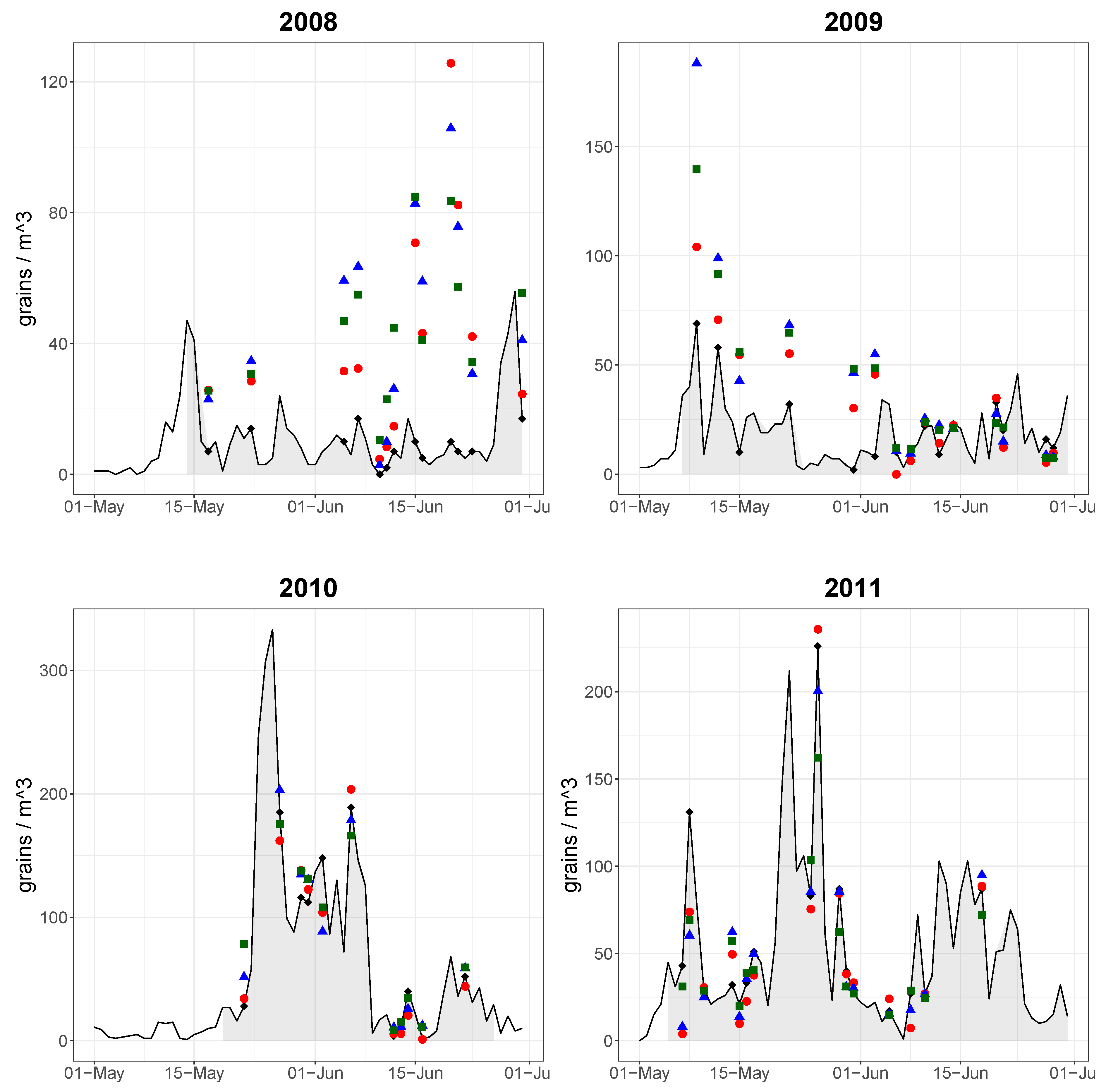
The aim was to compare the aforementioned methods in order to see their ability to impute data properly for the observation station in Farmacia (most central location available), by inferring airborne pollen counts at one station based on the levels measured in its surroundings. In order to do so, series with 10%, 20%, and 30% of missing data points were generated and then used as a test set to check the estimations. However, as we can see in Figure 1, airborne pollen time series are a particular kind of series where during most of the year, pollen counts are either nonexistent or very low. For this reason, a stratified random sample was drawn based on the criteria of an observation belonging to a peak or off-peak pollen season.
There is no general consensus about the definition of the pollen season, and hence, season dates might differ according to their definition [11]. This notwithstanding, in Spain, the first symptoms are observed over 25 grains/m 3 [33]. Accordingly, this level is selected to define the boundary dates of the main pollen season as the first and the last day that 25 grains/m 3 are observed, corresponding to the start and the end of the peak season, respectively. Thus, every random sample drawn would include X% of observations from the peak season and X% from the off-peaks season, X { 10 , 20 , 30 } .
For each percentage of missing data points, a 10-fold cross-validation was run to cover the full dataset. Subsequently, the GP and CNN algorithms were trained and tested against the corresponding test set. Since IDW is an unsupervised method, meaning that there is no need to train the algorithm in order to extract the relations between pollen counts at different locations and the control station of Farmacia, it was used as a benchmark to evaluate the Gaussian process and the neural network. For the Gaussian process regression, a dot product covariance function k ( x i , x j ) = σ 0 2 + x i · x j was used along with a noise level estimation σ 2 δ ( x i , x j ) [31] where δ ( x i , x j ) is the Kronecker delta function.
In order to parse the pollen counts through the CNN as the input, at each time t, the seven locations surrounding location i and the pollen observations p i were transformed into a 3 × 3 matrix, as seen in Equation (2), which in turn was transformed into a 5 × 5 matrix (Equation (2)) by adding zeros in order to capture the contributions of the individual locations and enrich the information flow through the network. Thus, by using a 2 × 2 filter with a stride equal to one, we ensured the parsing of an individual location, as seen in Figure 2 with element X 11 of the input matrix:
[ p 1 , p 2 , p 3 , p 4 , p 5 , p 6 , p 7 ] t 0 0 0 0 0 0 p 1 p 2 p 3 0 0 p 4 p 5 p 6 0 0 p 7 0 0 0 0 0 0 0 0 t
Given the aforementioned setup, with 14 filters, it would be sufficient to cover the full feature map without taking into account the last two filters, which would result in 0 (Figure 2). However, the generalization ability of CNNs is not based on limiting the number of parameters [34], and with an incremental experiment, 32 filters are adequate to solve this problem. As a final step, the filters were fully connected to a 5 neuron layer, which at the same time was connected to the output. CNNs usually suffer from an abrupt increment of the number of parameters as their complexity, in terms of topology, increases. Thus, it is common to include a pooling layer in order to reduce the number of parameters. Since the architecture proposed was fairly simple, adding this kind of layer was avoided, as the number of parameters was already small.
Figure 1 shows the particular nature of airborne pollen time series, with a high presence of observations equal or close to 0, especially outside the main pollen season. This may lead to what it is know as dead neurons, which results in the weights being equal to 0, since the amount of information from the inputs is limited. To avoid this situation, the network was trained using a “LeakyReLu” activation function ( α = 0.1 ) along with the Adam optimization algorithm [35] instead of the traditional stochastic gradient descent. A learning rate α = 0.001 , an exponential decay of β 1 = 0.9 , and β 2 = 0.999 were used to train the network over 60 epochs.

3. Results

The study was based on removing data points from the pollen observation station located at the Faculty of Pharmacy (Farmacia). Table 1 shows the average 10-fold RMSE and standard deviation for each percentage of observations subtracted from the time series. As mentioned in Section 2.3, the proportions of missing data were equally selected within and outside the main pollen season.
When removing 10% of the data points, the CNN provided a more accurate estimation, both during the peak and off-peak season, with an RMSE equal to 39.89 and 4.53 grains per square meter, respectively. These quantities were compared to an RMSE of 42.44 using Gaussian process regression and 43.97 obtained by IDW. The differences were closer during the off-peak season with 5.07 and 5.36 for GP and IDW, respectively. This situation was expected since, on the one hand, there were more observations outside the main pollen season and, on the other, airborne pollen concentrations were close to zero. Additionally, the stability of the estimations seemed higher for the CNN given the lowest standard deviation of the results.
CNN also improved the accuracy of other methods, both during the peak and off-peak season, when 20% of the observations were removed. With respect to the peak season, the CNN performed 10% better than IDW. This accuracy went to 5% better when compared to GP. In this case, as happened when removing 30% of the observations, the standard deviation was higher than that obtained by IDW. This behavior was expected since in computational intelligence models, the principle of the more data, the better applies in general. Still, the differences were residual.
Figure 3 shows the estimation of all three methods for the peak season during sample years 2008 to 2011. It can be clearly seen that the CNN (red circle) tended to adjust better to sudden peaks in concentrations. Furthermore, it managed to mitigate the influence of extreme observations from other locations, as it did not overestimate as much as the other two methodologies. This situation was demonstrated both in 2009 and 2011, where all models estimated an airborne concentration over 100 grains/m 3 , while the true observation was closer to 50 grains/m 3 .
One of the well known disadvantages of neural networks is the training execution times. For this reason, the training times were tracked (Table 2) to have a fair comparison in every aspect. For this analysis, IDW was discarded since it is a deterministic method, which was not comparable, in terms of time performance, to the other two. Intuitively, the more data removed, the shorter the execution times, as the training set decreased in size. We can see a certain stability in CNN time performance when compared to the Gaussian process consuming on average about 10% of the time of the GP in the training process.

4. Discussion

As we saw in Section 3, the competitive advantage of using CNNs to impute airborne pollen concentrations was clear. In terms of accuracy, both the Gaussian process and the CNN performed better than the inverse distance weighting method (Table 1). At the same time, both models could be extended by including a temporal dimension.
In order to provide insightful results, these were reported based on whether the observations belonged to the main pollen season or not. The main pollen season, or peak season, was defined using a threshold approach [36] of 25 grains/m 3 . This threshold differed from the literature based on the study region and pollen genus. However, the work in [37] concluded that Poaceae is ranked highest in terms of allergic significance, and the work in [10] established a threshold of 25 grains/m 3 for Plantago pollen. Furthermore, high pollen concentration thresholds might lead to very short peak seasons and consequently few test points.
During the main peak pollen season, all models suffered from the influence of extreme values in other locations (Figure 3), resulting in an overestimation of the concentrations at the target location. However, this influence was mitigated by the CNN due to the increase in the number of filters, which increased the model’s generalization.
During off-peak periods, the differences between the techniques proposed were marginal, but regarding their practical application, these observations were not as important, since they did not imply a high risk for the allergic population. There is no consensus about how much missing data is allowed in order to have unbiased statistical analyses when using inference models [14,15], the cutoff values being around 10% depending on the dataset. This was the reason why 10%, 20%, and 30% of missing data were selected. As a consequence, an increase of the number of filters used in the CNN topology was necessary to provide the generalization of the estimations as proven by the results. However, the larger the amount of missing data, the smaller the number of training observations, which negatively influences the learning process of the CNN. This explains why a decrease in the accuracy was obtained as a result.
Even though only pollen observations were used in this study, mainly to compare the proposed solution with the benchmark IDW, the CNN provided the flexibility to include meteorological measures or predictions as input variables. There is evidence that including such variables [12,24] improves the estimations of airborne pollen concentrations. Moreover, these variables serve as a differential factor to mitigate under- and over-estimation of sudden high peaks during the main pollen season. On the other hand, the simplicity of the topology of the proposed solution was lost. As a consequence, execution training periods increased as the number of hyper-parameters increased. This is a well known drawback of machine learning models; however, the applied method performed better compared to the others tested, mainly by computation time (Table 2), and is expected to outperform them significantly when additional co-factors are used, such as meteorological variables.

5. Conclusions

In this study, we tackled the problem of the spatial imputation of missing values for pollen time series in Madrid. We proposed the use of convolutional neural networks and conducted a comparison with two traditional geoimputation techniques, inverse distance weighting and Gaussian process regression. The CNN’s competitive advantage was shown both in terms of accuracy and execution times.
The results show that it is possible to apply this technique to fields outside computer vision and linguistics. Field experts can take advantages of the potential of CNNs and their application to spatial imputation. Even though the results were promising, they could be improved by including meteorological measures or predictions in the model, yet increasing the computational cost and complexity. This notwithstanding, it was also intended to increase the awareness of the advantages and disadvantages of such a technique.

Author Contributions

R.N.: conceptualization, methodology, software, formal analysis, investigation, writing-m –original draft, and visualization. J.L.A.: writing, review editing, and supervision.

Funding

This research received no external funding.

Acknowledgments

Pollen data were kindly provided by Patricia Cervigón (Palinocam network, Comunidad de Madrid) and Montserrat Gutiérrez Bustillo (Department of Botany, Complutense University of Madrid).

Conflicts of Interest

The authors declare no conflict of interest.

References

  1. De Weger, L.A.; Bergmann, K.C.; Rantio-Lehtimaki, A.; Dahl, A.; Buters, J.; Déchamp, C.; Belmonte, J.; Thibaudon, M.; Cecchi, L.; Besancenot, J.P.; et al. Impact of Pollen. In Allergenic Pollen; Sofiev, M., Bergmann, K.C., Eds.; Springer: Dordrecht, The Netherlands, 2013; pp. 161–215. [Google Scholar] [CrossRef]
  2. Lake, I.; Jones, N.; Agnew, M.; Goodess, C.; Giorgi, F.; Lynda, H.L.; Semenov, M.; Solmon, F.; Storkey, J.; Vautard, R.; et al. Erratum: “Climate Change and Future Pollen Allergy in Europe”. Environ. Health Perspect. 2018, 126. [Google Scholar] [CrossRef] [PubMed]
  3. Sabariego, S.; Cuesta, P.; Fernández-González, F.; Pérez-Badia, R. Models for forecasting airborne Cupressaceae pollen levels in central Spain. Int. J. Biometeorol. 2012, 56, 253–258. [Google Scholar] [CrossRef] [PubMed]
  4. Smith, M.; Emberlin, J. A 30-day-ahead forecast model for grass pollen in north London, UK. Int. J. Biometeorol. 2006, 50, 233–242. [Google Scholar] [CrossRef] [PubMed]
  5. Silva-Palacios, I.; Fernández-Rodríguez, S.; Durán-Barroso, P.; Tormo-Molina, R.; Maya-Manzano, J.; Gonzalo-Garijo, A. Temporal modelling and forecasting of the airborne pollen of Cupressaceae on the southwestern Iberian peninsula. Int. J. Biometeorol. 2016, 60, 1509–1517. [Google Scholar] [CrossRef]
  6. Schaber, J.; Badeck, F.W. Physiology-based phenology models for forest tree species in Germany. Int. J. Biometeorol. 2003, 47, 193–201. [Google Scholar] [CrossRef]
  7. Navares, R.; Aznarte, J. Forecasting the Start and End of Pollen Season in Madrid; Springer International Publishing: Berlin/Heidelberg, Germany, 2017; Chapter 26; pp. 387–399. [Google Scholar]
  8. Puc, M. Artificial neural network model of the relationship between Betula pollen and meteorological factors in Szczecin (Poland). Int. J. Biometeorol. 2011, 56, 395–401. [Google Scholar] [CrossRef]
  9. Castellano-Méndez, M.; Aira, M.J.; Iglesias, I.; Jato, V.; González-Manteiga, W. Artificial neural networks as a useful tool to predict the risk level of Betula pollen in the air. Int. J. Biometeorol. 2005, 49, 310–316. [Google Scholar] [CrossRef]
  10. Iglesias-Otero, M.A.; Fernández-González, M.; Rodríguez-Caride, D.; Astray, G.; Mejuto, J.C.; Rodríguez-Rajo, F.J. A model to forecast the risk periods of Plantago pollen allergy by using ANN methodology. Aerobiologia 2015, 31, 201–211. [Google Scholar] [CrossRef]
  11. Navares, R.; Aznarte, J. Predicting the Poaceae pollen season: six month-ahead forecasting and identification of relevant features. Int. J. Biometeorol. 2016. [Google Scholar] [CrossRef]
  12. Navares, R.; Aznarte, J. What are the most important variables for Poaceae airborne pollen forecasting? Sci. Total Environ. 2016, 579, 1161–1169. [Google Scholar] [CrossRef]
  13. Oteros, J.; Sofiev, M.; Smith, M.; Clot, B.; Damialis, A.; Prank, M.; Werchan, M.; Wachter, R.; Weber, A.; Kutzora, S.; et al. Building an automatic pollen monitoring network (ePIN): Selection of optimal sites by clustering pollen stations. Sci. Total Environ. 2019, 688, 1263–1274. [Google Scholar] [CrossRef]
  14. Schafer, J.L. Multiple imputation: A primer. Stat. Methods Med. Res. 1999, 8, 3–15. [Google Scholar] [CrossRef] [PubMed]
  15. Bennett, D. How can I deal with missing data in my study? Aust. N. Z. J. Public Health 2001, 25, 464–469. [Google Scholar] [CrossRef] [PubMed]
  16. Shepard, D. A Two-dimensional Interpolation Function for Irregularly-spaced Data. In Proceedings of the 23rd ACM National Conference, Las Vegas, NV, USA, 27–29 Auguest 1968; ACM: New York, NY, USA, 1968; pp. 517–524. [Google Scholar] [CrossRef]
  17. Matheron, G. Principles of geostatistics. Econ. Geol. 1963, 58, 1246–1266. [Google Scholar] [CrossRef]
  18. Kordon, A.K. Competitive Advantages of Computational Intelligence. In Applying Computational Intelligence: How to Create Value; Springer: Berlin/Heidelberg, Germany, 2010; pp. 233–256. [Google Scholar] [CrossRef]
  19. Lecun, Y.; Bottou, L.; Bengio, Y.; Haffner, P. Gradient-based learning applied to document recognition. Proc. IEEE 1998, 86, 2278–2324. [Google Scholar] [CrossRef]
  20. Krizhevsky, A.; Sutskever, I.; Hinton, G.E. ImageNet Classification with Deep Convolutional Neural Networks. In Advances in Neural Information Processing Systems 25; Pereira, F., Burges, C.J.C., Bottou, L., Weinberger, K.Q., Eds.; Curran Associates, Inc.: Makati, Philippines, 2012; pp. 1097–1105. [Google Scholar]
  21. Gehring, J.; Auli, M.; Grangier, D.; Yarats, D.; Dauphin, Y.N. Convolutional Sequence to Sequence Learning. In Proceedings of the 34th International Conference on Machine Learning, Sydney, Australia, 6–11 August 2017; Precup, D., Teh, Y.W., Eds.; PMLR: Sydney, Australia, 2017; Volume 70, pp. 1243–1252. [Google Scholar]
  22. Smith, S.W. The Scientist and Engineer’s Guide to Digital Signal Processing; California Technical Publishing: San Diego, CA, USA, 1997. [Google Scholar]
  23. Nowosad, J. Spatiotemporal models for predicting high pollen concentration level of Corylus, Alnus, and Betula. Int. J. Biometeorol. 2016, 60, 843–855. [Google Scholar] [CrossRef]
  24. Navares, R.; Aznarte, J.L. Forecasting Plantago pollen: improving feature selection through random forests, clustering, and Friedman tests. Theor. Appl. Climatol. 2019. [Google Scholar] [CrossRef]
  25. Zewdie, G.K.; Lary, D.J.; Levetin, E.; Garuma, G.F. Applying Deep Neural Networks and Ensemble Machine Learning Methods to Forecast Airborne Ambrosia Pollen. Int. J. Environ. Res. Public Health 2019, 16, 1992. [Google Scholar] [CrossRef]
  26. Sevillano, V.; Aznarte, J.L. Improving classification of pollen grain images of the POLEN23E dataset through three different applications of deep learning convolutional neural networks. PLoS ONE 2018, 13, e0201807. [Google Scholar] [CrossRef]
  27. Khanzhina, N.; Putin, E.; Filchenkov, A.; Zamyatina, E. Pollen grain recognition using convolutional neural network. In Proceedings of the European Symposium on Artificial Neural Networks, Computational Intelligence and Machine Learning, Bruges, Belgium, 25–27 April 2018. [Google Scholar]
  28. Galán Soldevilla, C.; Cariñanos González, P.; Alcázar Teno, P.; Domínguez Vílches, E. Manual de Calidad y Gestión de la Red Española de Aerobiología; Universidad de Córdoba: Córdoba, Spain, 2007. [Google Scholar]
  29. Tobler, W.R. A Computer Movie Simulating Urban Growth in the Detroit Region. Econ. Geogr. 1970, 46, 234–240. [Google Scholar] [CrossRef]
  30. Murphy, K.P. Machine Learning: A Probabilistic Perspective, 1st ed.; MIT Press: Cambridge, MA, USA, 2012. [Google Scholar]
  31. Edward Rasmussen, C.; Bousquet, O.; von Luxburg, U.; Rätsch, G. Gaussian Processes in Machine Learning. In Advanced Lectures on Machine Learning: ML Summer; Springer: Berlin/Heidelberg, Germany, 2004; Volume 3176. [Google Scholar] [CrossRef]
  32. Gamboa, J.C.B. Deep Learning for Time-Series Analysis. arXiv 2017, arXiv:1701.01887. [Google Scholar]
  33. Rodríguez-Rajo, F.; Frenguelli, G.; Jato, M. Effect of air temperature on forecasting the start of the Betula pollen season at two contrasting sites in the south of Europe (1995–2001). Int. J. Biometeorol. 1983, 47, 117–125. [Google Scholar]
  34. Zhang, C.; Bengio, S.; Hardt, M.; Recht, B.; Vinyals, O. Understanding deep learning requires rethinking generalization. arXiv 2016, arXiv:1611.03530. [Google Scholar]
  35. Kingma, D.P.; Ba, J. Adam: A Method for Stochastic Optimization. arXiv 2014, arXiv:1412.6980. [Google Scholar]
  36. Jato, V.; Rodríguez-Rajo, F.J.; Alcázar, P.; Nuntiis, P.D.; Galán, C.; Mandrioli, P. May the definition of pollen season influence aerobiological results? Aerobiologia 2006, 22, 13–25. [Google Scholar] [CrossRef]
  37. Peternel, R.; Srnec, L.; Culig, J.; Hrga, I.; Hercog, P. Poaceae pollen in the atmosphere of Zagreb (Croatia), 2002–2005. Grana 2005, 45, 130–136. [Google Scholar] [CrossRef]
Figure 1. Selected stations with Poaceae pollen concentrations capped at 100 grains/m 3 (left). Distribution of the locations in the region of Madrid (right).
Atmosphere 10 00717 g001
Figure 2. Convolutional neural network.
Atmosphere 10 00717 g002
Figure 3. Sample estimation points during peak seasons (grey area) in 2008 to 2011 representing CNN (red circle), GPR(blue triangle), and IDW (green square). The missing observed data points are represented by a black diamond.
Atmosphere 10 00717 g003
Table 1. Average and standard deviation (in parenthesis) of the RMSE per percentage of missing data and methodology.
% of MissingPeak SeasonOff-Peak SeasonAll
IDWGPCNNIDWGPCNNIDWGPCNN
10%43.9742.4439.895.365.074.5318.0217.4116.46
(5.84)(8.56)(5.25)(0.91)(1.09)(0.98)(2.05)(3.02)(2.02)
20%41.5539.6937.355.765.244.8017.2616.4315.42
(3.95)(4.72)(4.21)(1.50)(1.55)(1.20)(1.57)(1.80)(1.48)
30%42.7941.5040.146.455.925.4017.8717.2416.60
(3.77)(4.20)(4.05)(0.68)(0.79)(1.15)(1.52)(1.66)(1.60)
Table 2. Average and standard deviation (in parenthesis) of the 10-fold execution time in seconds per percentage of missing data.
GPCNN
10% missing243.3817.47
(10.56)(0.66)
20% missing171.2215.91
(18.00)(0.64)
30% missing148.1215.55
(24.19)(1.65)

