Abstract
Using the ERA-Interim total column ozone data, the spatial distributions of the long-term mean of the global total ozone in summer are analyzed. The results demonstrate that there are three midlatitude ozone “valleys” on earth—they are centered over the Tibetan Plateau (TIP), the Rocky Mountains (ROM), and the Southwest Pacific (SWP), respectively. The interdecadal variations of the three ozone valleys are positively modulated by the solar radiation, and the TIP ozone’s correlation with the solar radiation gets maximized with a two-year lag. The interdecadal variation of the SWP ozone valley has a significantly negative relationship with the Pacific Decadal Oscillation (PDO) and the South Pacific quadrupole (SPQ). Warm sea surface temperature anomalies (SSTAs) associated with the SPQ strengthen the vertical ascending motion, which dilutes the high concentration ozone at high altitudes. The interdecadal variation of the ROM ozone valley is positively correlated with the PDO, leading by three years. The ROM ozone content is also modulated by SSTAs in the Indian Ocean basin (IOB) by the circumglobal teleconnection (CGT). The observed regional SSTAs can exert a significant impact on the regional and even global circulation, via which the ozone content in midlatitudes also varies.
1. Introduction
Ozone is one of the most important components in the atmosphere. Ozone in the stratosphere can absorb short-wave radiation, and thus plays a vital role in balancing stratospheric energy [1,2,3] and protecting the ecosystem [4]. Animals and plants cannot live without its protections [5]. Great ozone depletion was found over the South pole [6] and North pole [7], and it is of high value to study the ozone holes that might destroy the ecosystem and threaten human lives [8,9,10].
Besides the poles, ozone depletion is also found over middle latitudes. Zhou et al. [11] discovered the ozone valley over the Tibetan Plateau (TIP) using the Total Ozone Mapping Spectrometer (TOMS) satellite data from 1979 to 1991. Later studies [12,13,14] successively confirmed the existence of the ozone valley over the TIP. Another ozone low center was found in the upper stratosphere over the TIP by Guo et al. [15] in Stratospheric Aerosol and Gas Experiment (SAGE) II data. Subsequently, Guo et al. [16] confirmed the double-core structure of the ozone valley over the TIP in Aura Microwave Limb Sounder (MLS) data. The population of the midlatitudes is denser than that of the polar regions, so it is more meaningful to study the formation mechanism and change mechanism of ozone valleys over middle latitudes.
The mechanism of ozone valley formation has been studied widely. Both the air column shrinkage due to the high altitude of the plateau and the air column expansion by the large heating rate of the plateau in the boreal summer are responsible for the formation of the ozone valley [17,18,19]. Zhou et al. [11] speculated that the physicochemical processes related to convection activities in the South Asian high contribute to the formation of the ozone valley over the TIP. Su and Wang [20] found the movement of the South Asian high is related to atmospheric ozone changes. Using reanalysis data and satellite data, Zhou and Chen [21] found that when the South Asian high is enhanced, the isothermal surface of 120–30 hPa rises, corresponding to an anomalous updraft. This updraft transports the low-ozone air upward, thereby reducing the ozone concentration. In addition, changes in tropopause height and large-scale circulation play a key role in the ozone valley over the TIP in the upper troposphere and lower stratosphere (UTLS) [21,22,23,24,25]. Most studies tend to indicate that the formation of the ozone valley over the TIP is more closely related to dynamic influence than chemical influence [15,18,19,21,26,27,28,29]. However, for the ozone valley over the TIP in the upper stratosphere, chemistry may be more important [16,30,31].
The change mechanism of the ozone valley mainly includes ozone-depleting substances produced by human activities [32,33], volcanic activity [34,35], solar radiation [36,37], Quasi-Biennial Oscillation (QBO) [38,39], and El Niño-Southern Oscillation (ENSO) [40,41]. The impact of QBO and ENSO on ozone on the interannual timescale has been widely reported, but there are still fewer investigations on the interdecadal variations of the ozone valley. Moreover, the research on the ozone valley is mainly concentrated on the TIP with satellite data, but there may exist other ozone valleys in midlatitudes. Given that the time period for a single set of satellite data is too short to study its interdecadal variation, an integral dataset might be adopted. For example, varieties of ozone data from satellite instruments are assimilated in ERA-Interim reanalysis data. Previous studies [42,43] have compared ERA-Interim with satellite data and found that they have a very consistent change in total column ozone. The relative standard error of them does not exceed ±5 DU (about 3%). In recent years, ERA-Interim reanalysis ozone data have been widely used [44,45,46]. Therefore, we use the ERA-Interim total column ozone data to locate the midlatitude ozone valleys in summer, to explore their interdecadal variations, and to establish the relationship between ozone valleys and solar cycles or between oceanic variations and ozone on the decadal timescale.
2. Data and Method
The ERA-Interim monthly mean data of total column ozone were used, and the time span was from January 1979 to December 2017. The unit of total column ozone in ERA-Interim is . The unit was converted from to the standard ozone units, DU (1 DU = 2.1415 × 10⁻⁵ ). We mainly focused on the midlatitudes from 30–60° N/S in summer. Northern Hemisphere summer is June, July, and August, while Southern Hemisphere summer is December, January, and February. From 1979 to 2017, there were 39 complete summers in the Northern Hemisphere and 38 complete summers in the Southern Hemisphere.
The ozone valley index is defined as the area-weighted zonal deviation of the low ozone region, respectively. We refer to the three indices as the Tibetan Plateau Index (TPI), the Rocky Mountains Index (RMI), and the Southwest Pacific Index (SWPI). They were smoothed with an 11 year moving slide, which is commonly used in the study of interdecadal variability [47,48], so the fluctuations with a cycle less than or equal to 10 years were filtered out. The long-term trends of the three indices were subtracted from the 11 year running mean data to obtain the “pure” interdecadal components,
In Equation (1), is the interdecadal variation, x is the ozone 11 year running mean valley index, and is the least squares linear trend of the long-term indexes.
We searched for the main factors that cause the interdecadal variations of the ozone valley index by studying solar radiation and ocean variability first in this paper. For solar radiation, we used F10.7 solar radiation daily data. It is the solar radiant flux at 10.7 cm, or 2800 MHz, in units of SFU (1 SFU = 10−22 W m−2 Hz−1). F10.7 is a good measure of general solar activity [49]. Previous research has established a dynamic relationship between the Pacific Decadal Oscillation (PDO) and the stratosphere [50,51,52,53]. For the possible modulation of the ozone by the PDO on the interdecadal timescale, the monthly PDO data provided by the Joint Institute for the Study of the Atmosphere and Ocean (JISAO) were used (research.jisao.washington.edu/pdo/PDO.latest). There are still few studies on the relationship between ocean and ozone on the interdecadal timescale. The Hadley Center Sea Ice and SST dataset (HadISST) [54] on a 1° × 1° spatial grid was used to search for key oceanic regions for the three ozone valleys. We used the ERA-Interim reanalysis data to diagnose the atmospheric circulation. This reanalysis dataset has a horizontal resolution of 1.5° × 1.5° and 37 pressure levels from 1000–1 hPa.
3. Midlatitude Ozone Valleys in Summer
3.1. Zonal Asymmetry of Total Ozone
By subtracting the zonal mean, the spatial distribution of the zonal mean ozone can better highlight the zonal asymmetry of total ozone. Figure 1a shows the zonal deviation field of midlatitude total ozone in the Northern Hemisphere during the boreal summer. The shaded area denotes the zonal deviation smaller than −10 DU. It can be seen that there are two main low centers for ozone in the Northern Hemisphere, one over the TIP and the other over the Rocky Mountains (ROM). The altitude of the TIP is 3–5 km, and the altitude of the ROM is 2–3 km. The high altitude shortens the local air column, reducing the total ozone. The TIP is higher than the ROM, and the ozone valley is deeper and the coverage for the former is wider than the latter. This reflects that the terrain is one of the most important factors for the formation of the ozone valleys. Similarly, Figure 1b shows the zonal deviation of total ozone in the Southern Hemisphere summer. There is a low ozone area in the Southwest Pacific (SWP). Unlike the Northern Hemisphere, this low center is located over the ocean, indicating that the main formation mechanism for this the ozone valley is different from the other two ozone valleys in the Northern Hemisphere. Three ozone valley indices are calculated (red boxes shown in Figure 1): the TPI is the zonal mean deviation averaged over 28–38° N, 79–101° E; the RMI is averaged over 38–50° N, 114–102° W; the SWPI is averaged over 59–51° S, 178–146° W.
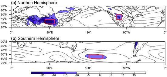
Figure 1.
Long-term mean (climatology) of the midlatitude zonal deviation of the total ozone in the (a) Northern and (b) Southern Hemisphere summer during 1979–2017 (units: DU). The three boxes mark the ozone valleys: 28–38° N, 79–101° E; 38–50° N, 114–102° W; 59–51° S, 178–146° W.
3.2. Interdecadal Variations of the Three Ozone Valleys
The interannual variations of TPI, RMI, and SWPI are much larger than the interdecadal component. To thoroughly study the interdecadal component, an 11 year running average was performed for TPI, RMI, and SWPI, so that the interannual component with a period of <10 years was filtered out. As shown in Figure 2a–c, the black dotted curve is unfiltered data, the black solid line is the 11 year running average of them, and the red solid line is the trend. The trend of TPI do not pass the significance test at the 0.1 confidence level. The trend of RMI (0.18 DU/a) and SWPI (0.17 DU/a) are, respectively, above the 0.01 and 0.05 confidence level. Since the ozone valley indices are negative, the rising trend represents their significant weakening trend. The interdecadal variation in Figure 2d–f is the difference between the 11 year running average and its trend. The interdecadal variation of TPI () changes little in the late 20th century, with a positive phase from 2000 to 2008, followed by a negative phase. RMI’s interdecadal variation () is similar to the SWPI’s interdecadal variation (). They show a positive phase from 1990 to 2005 and a negative phase in other time periods. Among the three ozone valley indices, TPI has the slowest rise rate and the smallest interdecadal variation (σ = 0.34). The interdecadal variation of SWPI is the largest (σ = 1.48), followed by RMI (σ = 0.66). In contrast, SWPI might be more easily affected by the underlying ocean than the ozone valleys over continents.
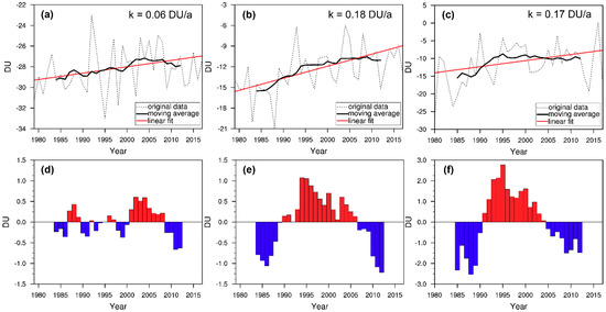
Figure 2.
(a) The Tibetan Plateau Index; (b) the Rocky Mountains Index; (c) the Southwest Pacific Index. The dotted line is the raw data, the red line denotes the trend of the original raw data, and the black solid curve is the 11 year running mean of the raw data. (d–f) Interdecadal component of (a–c).
4. Possible Reasons for Interdecadal Variations of the Midlatitude Ozone Valleys
This section examines the possible relationship between the 11 year solar cycle or the ocean sea surface temperature (SST) and the interdecadal variations of three ozone valleys. Solar radiation can affect ozone through a photochemical reaction, whereas the interdecadal variation of the ocean SST can dynamically affect the troposphere–stratosphere exchange and therefore the ozone.
4.1. Solar Radiation
Solar radiation generally exhibits an 11 year cycle, but the actual lifetime of each solar cycle is different. In order to demonstrate the robustness of the moving average, we smoothed the F10.7 data with the window of 9, 11, and 13 years, and the results were roughly the same (i.e., the correlations between 11 year moving average and 9 and 13 year moving averages were 0.5972 and 0.5966, and they respectively pass the 0.001 significance level). Figure 3 shows the boreal summer and austral summer solar radiations, as well as their 11 year running means. It can be seen from Figure 3 that the global summer solar radiation has a declining trend. By comparing the interdecadal variations of the three ozone valley indices (, , ) with the interdecadal variation of solar radiation ( in boreal summer, in austral summer), it can be seen that the phases of and , and of and are similar—the negative phase in the early stage, and the positive phase in the 1990s, followed by a negative phase. The phase of follows the solar radiation with about a two-year lag.
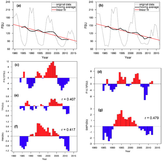
Figure 3.
(a) The year-by-year time series of boreal summer solar radiation. (b) The year-by-year time series of austral summer solar radiation. The dotted line is the raw data, the red line denotes the trend of the original raw data, and the black solid curve is the 11 year running mean of the raw data. (c,d) Interdecadal component of (a,b). (e–g) Interdecadal component of Tibetan Plateau Index (TPI), Rocky Mountains Index (RMI), Southwest Pacific Index (SWPI).
In order to further study the influence of the solar radiation on the interdecadal variation of the ozone valleys in the three regions, we normalized and calculated the correlation coefficient between , , and ; and , respectively. The correlation coefficient between normalized and is 0.407 (>α0.05 = 0.367, n = 29). The correlation coefficient between normalized and is 0.417 (>α0.05 = 0.367, n = 29). These indicate the importance of the 11-year solar cycle for the interdecadal variation of the TIP and ROM ozone valley. Moreover, the correlation coefficient between normalized and is even larger, 0.479 (≥α0.01 = 0.479, n = 28).
The maximum correlation between the ozone valleys and the solar cycle might appear with several-year lags. The lead/lag correlation between the normalized three ozone valleys and solar cycle is shown in Figure 4. The correlation coefficient between normalized and reaches a maximum (~0.812) at a lag of two years, which might indicate that more than half of the interdecadal variability of the TIP ozone valley is explained by the solar cycle, as shown in Figure 4a. Different from the TIP, the ROM ozone is less correlated with the solar cycle, and the maximum correlation appears when the ozone and the solar cycle are concurrent without any lag, as shown in Figure 4b. Similarly, the maximum correlation between the solar cycle and SWPI also appear when they are concurrent, as shown in Figure 4c.
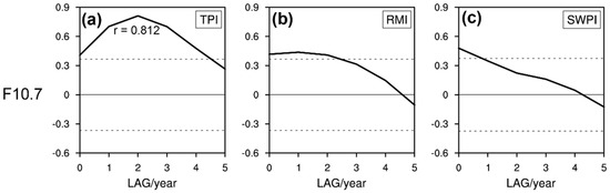
Figure 4.
Lag correlations between (a) , (b) and ; (c) between and . The abscissa is ozone valley’s lags. The horizontal dashed lines mark the 95% confidence level.
The results show that the interdecadal variation of the ozone valleys can be modulated by the solar radiation. The positive correlation between the solar cycle and regional ozone might indicate that the solar cycle can affect the physicochemical reactions of ozone and its product in the atmosphere [55]. During solar maximum, the tropical stratosphere is anomalously warm, which in turn increases the air stability and weakens the tropical upwelling, favoring an increase in ozone in lower latitudes [56,57].
4.2. Pacific Decadal Oscillation
Since all the three ozone valleys are located near the Pacific Ocean, the correlation between the Pacific Decadal Oscillation (PDO) and ozone was also examined. The PDO has a quasi 10 year cycle for a dipole SST pattern between the North Pacific and subtropical Pacific, viewed as a mode of ocean–atmosphere internal variability over the extratropical Pacific basin [52,58].
Figure 5 shows the 11 year running average and the interdecadal component of the PDO in the Northern and Southern Hemisphere summers, respectively. It can be seen from Figure 5a,b that both boreal and austral summer PDO shows a decreasing trend. By comparing the three ozone valley indices (, , ) and the interdecadal variation of PDO ( in boreal summer, in austral summer), it can be seen that the tends to be out of phase with the . However, the tends to be in phase with the , and the phase of the PDO seems to lead that of the by several years.
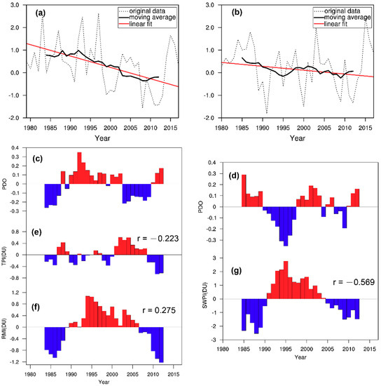
Figure 5.
(a) The year-by-year time series of boreal summer Pacific Decadal Oscillation (PDO). (b) The year-by-year time series of austral summer Pacific Decadal Oscillation (PDO). The dotted line is the raw data, the red line denotes the trend of the original raw data, and the black solid curve is the 11 year running mean of the raw data. (c,d) Interdecadal component of (a,b). (e–g) Interdecadal component of Tibetan Plateau Index (TPI), Rocky Mountains Index (RMI), Southwest Pacific Index (SWPI).
To quantify the possible influence of the PDO on the interdecadal variation of the three ozone valleys, the correlation coefficients between , , and , and between and were calculated. The correlation coefficient between normalized and is −0.223, which fails to pass the significance test at the 0.1 confidence level (i.e., , n = 29). The correlation coefficient between normalized and is −0.275, indicating the concurrent relationship between the ROM total ozone and PDO is weak (, n = 29). The correlation coefficient between normalized and is −0.569, above the 0.01 confidence level (, n = 28).
From the aforementioned analysis, it can be concluded that the interdecadal variations of the TPI and RMI might not be related to the concurrent PDO, although the SWPI has a strong concurrent correlation with PDO. The SWP ozone valley is situated over the Pacific and global SST can be modulated by the PDO [52]. We also tested the lead/lag correlation between the PDO and the midlatitude ozone valleys in Figure 6. It is seen once again that the TIP ozone valley is unrelated to the PDO at different lags, as shown in Figure 6a, but the ozone tends to be anomalously abundant over the ROM three years after the positive phase of the PDO, as shown in Figure 6b. Previous studies [59,60,61,62] have shown that the PDO can affect the North American climate, but its specific mechanism remains unclear. Zhang et al. [25] argue that ENSO events can excite planetary waves by tropical convection, which will propagate into the middle latitudes and give rise to Pacific–North American pattern (PNA), then affect the vertical distributions of ozone. According to Deser et al. [63], the PDO is likely not a single physical mode but rather the sum of several phenomena. The ENSO-derived variability of the PNA is hypothesized to be integrated and low-passed by the ocean to yield the decadal PDO pattern [64,65,66]. Different from the Northern Hemisphere summer ozone valleys, the impact of the PDO on the SWP ozone abundance is persistent with the lagged years from 0 to 4, as shown in Figure 6c.
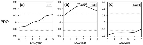
Figure 6.
As in Figure 4, but for the lead/lag correlation between the three ozone valleys and the PDO Index. (a) , (b) and ; (c) between and .
From the above, the impact of the solar cycle on the three hemispheric summer ozone valleys is uniform, with the concurrent correlation between the solar flux and ozone abundance around 0.4. In contrast, the PDO is shown to seldom impact the TIP ozone, and it mainly affects the ROM and SWP ozone valleys.
4.3. The Relationship between Global SST and Ozone Valleys
4.3.1. Extension to the Global SST
Although studies of the relationship between sea surface temperature and ozone on the interannual timescale have been widely reported [67,68], the decadal SST forcing responsible for the ozone variations are relatively seldom explored. Figure 7 shows the concurrent correlation coefficients between the three ozone valleys and the global SST, respectively. It can be seen from Figure 7a that the correlation between the global SST and TIP ozone is fairly weak, so this paper does not conduct in-depth analysis. In Figure 7b, the most significant region associated with RMI is located in the tropical Indian Ocean, and the correlation pattern largely resembles the Indian Ocean basin (IOB) mode [69]. The IOB mode is the leading empirical orthogonal function (EOF) of the tropical Indian Ocean sea surface temperature anomalies (SSTAs). However, the largest correlation for the Southern Hemisphere summer ozone valleys is situated over the South Pacific Ocean, exhibiting a zonal quadrupole, resembling the South Pacific quadrupole (SPQ) [70]. The SPQ is the second EOF mode of SSTAs in the extratropical South Pacific. Therefore, we applied an EOF analysis on the tropical Indian Ocean SST in boreal summer and the extratropical South Pacific SST in austral summer, respectively, so as to explore its relationship with the interdecadal variations of ozone valleys in ROM and SWP.
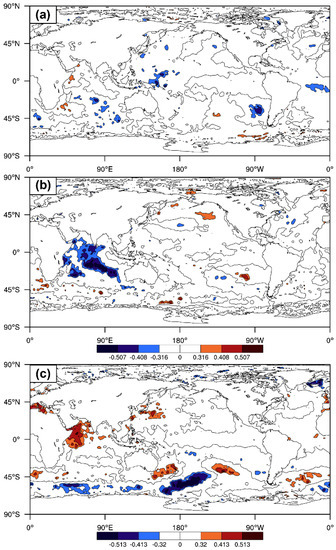
Figure 7.
Correlations between (a) Tibetan Plateau Index, (b) Rocky Mountains Index and boreal summer sea surface temperature (SST), and (c) between Southwest Pacific Index and austral summer SST. The shaded area marks the correlation at the 95%, 99%, and 99.9% confidence levels.
4.3.2. Remote Impact of IOB on RMI
Figure 8a shows the first EOF mode of the tropical Indian Ocean (40–100° E, 20° S–20° N) SSTAs in boreal summer, and the variance contribution is 53.2%. The SSTAs are uniform across the basin, and the standardized time series is defined as the IOB Index (IOBI), as shown in Figure 8b. The interdecadal variation of IOBI () is the 11 year running mean of the detrended IOB Index, as shown in Figure 8c. Comparing the timeseries of the filtered IOB and RMI indices, it is shown that the former tends to be out of phase with the latter phases. The correlation coefficient between normalized and is −0.805, above the 0.01 significance level (, n = 29).
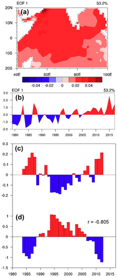
Figure 8.
(a) Spatial patterns of the leading empirical orthogonal function (EOF) of the tropical Indian Ocean SST in boreal summer. (b) Standardized time series of the leading EOF mode in (a). (c) The interdecadal component of (b). (d) The interdecadal component of the Rocky Mountains Index.
With observational analysis and model experiments, Yang et al. [71] concluded that that the SSTAs associated with the IOB can generate significant circumglobal teleconnection (CGT) [72] in the Northern Hemisphere summer midlatitude atmosphere, which has a strong influence on North American circulation [73]. A warm IOB can increase precipitation in south Asia through the enhanced Indian summer monsoon and induces an atmospheric heating source there. This new atmospheric heating source generates an upper-level anomalous high over west-central Asia, exciting the downstream wave train in the westerly waveguide, forming the CGT [71]. This pattern exhibits a zonal wavenumber 5 structure, locating across western Europe, west-central Asia, east Asia, north Pacific, and North America. Previous studies have shown that tropopause variations have a large impact on ozone and a lifting of tropopause height decreases total column ozone [24,74]. Descending of the tropopause height can cause an overall downward shift of ozone profiles and induce downward transport of ozone [18,25]. The stratospheric ozone concentration is usually greater than troposphere, thereby giving rise to total column ozone.
To further understand the interdecadal variations of RMI and its relationship with the tropical Indian Ocean SSTAs, interdecadal composite analysis was performed on the tropical SST and 200 hPa height in boreal summer. Three periods based on the phase of were selected: 1984–1989 (negative phase), 1990–2006 (positive phase), and 2007–2012 (negative phase), as shown in Figure 9. In the first and third periods, the is in its negative phase; the ozone valley over the ROM is strong, which is related to the IOB warming anomalies. Based on the 200 hPa height anomalies, there is an anomalous high over North America, suggesting the lift of tropopause height, thus deepening the ozone valley. It was found that the positions of four anomalous highs (black boxes) are very close to the CGT pattern, indicating the possible role of the CGT in redistributing ozone. During the second period, the phase of is positive, that is, the ozone valley is weak, which corresponds to a basin-wide cooling in the tropical Indian Ocean. The CGT pattern is in its negative phase; the North American low causes tropopause height decline and weakens the ozone valley. This indicates that the IOB can affect the interdecadal variations of the ozone valley in the ROM through tropopause height anomalies associated with the CGT.
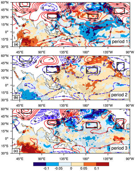
Figure 9.
Interdecadal composite analysis of the tropical sea surface temperature anomalies (SSTAs) (shadings; units: °C) and 200 hPa height anomalies (contours; units: gpm) in boreal summer. The dotted region marks the SSTAs at the 90% confidence level. Black boxes denote anomalous high/low corresponding with the circumglobal teleconnection (CGT). Three periods based on the phase of are selected: (a) 1984–1989 (negative phase); (b) 1990–2006 (positive phase); (c) 2007–2012 (negative phase).
4.3.3. Local Impact of South Pacific SST on the SWPI
Following Ding et al. [70], we also performed an EOF analysis for SSTAs of the extratropical South Pacific (20° S–60° S, 145° E–70° W) in austral summer. The second EOF mode is shown in Figure 10a, with the variance contribution of 12.5%. Spatial distribution exhibits a quadrupole-like structure, and the standardized time series is defined as the South Pacific quadrupole Index (SPQI) as shown in Figure 10b. The interdecadal component of SPQI () is out of phase with . The correlation coefficient between normalized and is −0.737, above the 0.01 confidence level (, n = 28), although the variance contribution of EOF2 to the total SST variance is low.
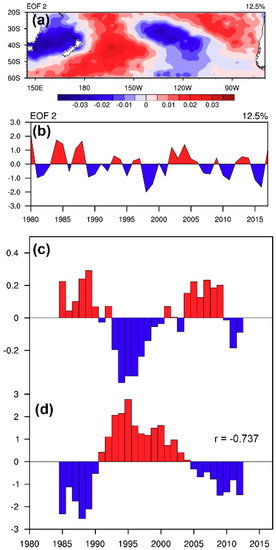
Figure 10.
(a) Spatial patterns of the leading EOF of the tropical Indian Ocean SST in boreal summer. (b) Standardized time series of the leading EOF mode in (a). (c) The interdecadal component of (b). (d) The interdecadal component of the Southwest Pacific Index.
Figure 11 shows the interdecadal composite analysis on the extratropical South Pacific SSTAs and 200 hPa height in austral summer. Three periods were selected based on the phase of : 1985–1990 (negative phase), 1991–2004 (positive phase), and 2005–2012 (negative phase). The is in its negative phase during the first and third periods, corresponding to positive SSTAs near the SWPI region. In the second period, the phase of is positive, and the local SSTAs are anomalously low. The composite SSTAs largely resemble the South Pacific quadrupole. In the first and third periods, there is an anomalous high at 200 hPa in the SWPI region, lifting high-altitude tropopause and deepening the ozone valley. During the second period, the local low center causes a high-altitude tropopause decrease and weakens the ozone valley.
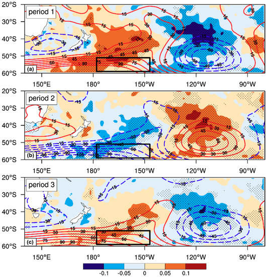
Figure 11.
Interdecadal composite analysis of the South Pacific SSTAs (shadings; units: °C) and 200 hPa height anomalies (contours; units: gpm) in austral summer. The dotted region marks the SSTAs at the 90% confidence level. The black box denotes the region of the Southwest Pacific Index. Three periods based on the phase of are selected: (a) 1985–1990 (negative phase); (b) 1991–2004 (positive phase); (c) 2005–2012 (negative phase).
Figure 12 shows the zonal cross-section of the circulation response in the three periods. During the first and third periods, the ozone valley over the SWP is strong, which is mainly related to the local warm SSTAs and the upwelling response, as shown in Figure 12a,c. This updraft favors the air exchange between ozone-poor air in the troposphere and ozone-rich air in the stratosphere. In the second period, the ozone valley is weak, corresponding to the local cold SSTAs and the anomalous downwelling, as shown in Figure 12b. In contrast, the ozone valley intensity and SSTAs in the first period are larger than those in the third period, and the corresponding vertical ascending motion in the first period is also stronger than that in the third period. Therefore, it is speculated that the positive SSTAs enhance the local ascending motion. Air masses with low ozone concentrations are lifted, diluting high-concentration ozone at high altitudes, deepening the ozone valley.
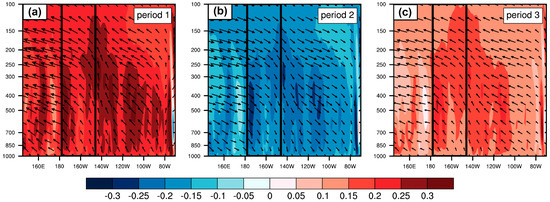
Figure 12.
Interdecadal composite analysis of zonal circulation in the 51–59° S latitude band. Filling color represents the vertical wind speed at pressure levels (−200 × omega; units: Pa/s). Black solid lines mark the west and east boundaries of the Southwest Pacific Index. Three periods based on the phase of are selected: (a) 1985–1990 (negative phase); (b) 1991–2004 (positive phase); (c) 2005–2012 (negative phase).
5. Summary
The ERA-Interim total column ozone data were employed to study the zonally asymmetric distribution of ozone in summer, whereby three ozone valleys were spotlighted, including the Tibetan Plateau valley, the Rocky Mountains valley, and the Southwest Pacific valley. Although the interannual relationship between ozone and global SST has been widely reported in the literature, the interdecadal variations of three ozone valleys and their relationship with the solar cycle and global SST are not well understood. The main conclusions in this study are as follows.
- The zonal distribution of total ozone in the midlatitudes is non-uniform. Three clear low centers were found, located over the Tibetan Plateau, Rocky Mountains, and Southwest Pacific, respectively. The latter two are significantly weakening.
- The interdecadal variations of three ozone valleys are significantly positively correlated with the solar radiation, which might imply that the solar cycle has a relatively uniform impact on the ozone abundance in the three valley regions. However, the solar cycle has a maximum impact on the Rocky Mountains Index, and Southwest Pacific Index without any time lag, but the TIP ozone’s response to the solar cycle gets maximized by lagging two years.
- The interdecadal variation of the Southwest Pacific Index can also be controlled by the Pacific Decadal Oscillation and the South Pacific quadrupole SST. Specifically, the Pacific Decadal Oscillation has a significantly negative correlation with the Southwest Pacific Index, which might be attributed to the impact of the Pacific Decadal Oscillation on global climate reported in previous studies [75,76]. The interdecadal variation of the Southwest Pacific Index is also negatively correlated with the South Pacific quadrupole SSTAs. When the Southwest Pacific Index is in the negative phase, indicating the strong ozone valley, the local sea is anomalously warm, corresponding to a positive South Pacific quadrupole Index; and vice versa. It is speculated that warm SST enhances the local ascending motion. Air masses with low ozone concentrations are lifted, diluting high-concentration ozone at high altitudes, deepening the ozone valley over the Southwest Pacific.
- The interdecadal variation of the Rocky Mountains Index is mainly associated with the Pacific Decadal Oscillation and Indian Ocean basin SSTAs. The Pacific Decadal Oscillation has a maximum impact on ROM ozone with a lag of three years. The interdecadal variation of RMI is negatively correlated with the Indian Ocean basin Index. When the Rocky Mountains Index is in the negative (positive) phase, most of the Indian Ocean presents a positive (negative) SSTA, and the 200 hPa circulation shows a high (low) anomaly center over North America, increasing (decreasing) tropopause height, thus the total column ozone reduces (rises).
We also used the raw Tibetan Plateau Index, Rocky Mountains Index, and Southwest Pacific Index to explore the relationship between the total ozone and solar radiation or ocean SSTs, but we found that their correlations were quite weak. The relationship between the solar radiation or ocean modes and the total ozone on the interdecadal timescale might not be applicable to the interannual timescale. However, factors determining the interannual variation of the ozone valleys are still not widely studied. There are still other decadal modes in the atmosphere–ocean system, like the decadal oscillation in the Southern Pacific [77] and Atlantic multidecadal oscillation [78]. The possible relationships and physical mechanisms between the total ozone and those modes also deserve further study in the future.
This study only considers two influencing factors—the 11 year solar cycle and the ocean SST modes. In addition, the projected ozone changes in the 21st century in different scenarios can also be explored by considering different pollutants [28]. The policies about energy saving and emission reduction all over the world have been widely recognized and put into action. The rising trend of total ozone indicates that ozone protection has worked. The global ozone recovery and its role in climate change are still under investigation [79].
Author Contributions
For conceptualization, D.G. and J.R.; methodology, L.L., W.Z. and Z.Z.; software, W.Z. and Z.Z.; validation, C.S., L.L. and J.R.; formal analysis, L.L. and Z.Z.; investigation, W.Z. and Z.Z.; resources, Y.S. and Z.T.; data curation, Z.Z.; writing—original draft preparation, Z.Z.; writing—review and editing, D.G. and J.R.; visualization, Z.Z.; supervision, D.G. and J.R.; project administration, D.G. and J.R.; funding acquisition, D.G. and F.Z.
Funding
This work was jointly supported by grants from the National Key Research and Development Project (2018YFC1505602), the Natural Science Foundation of China (91837311, 41675039, 41875048, 41705024), and the National Key Research and Development Program of China (2016YFC0202403, 2016YFA0602104).
Acknowledgments
We acknowledge the European Centre for Medium-Range Weather Forecasts (ECMWF) for providing the reanalysis data.
Conflicts of Interest
The authors declare no conflict of interest.
References
- Andrews, D.G.; Leovy, C.B.; Holton, J.R. Middle Atmosphere Dynamics; Academic Press: Cambridge, MA, USA, 1987; Volume 40. [Google Scholar]
- Zhang, F.; Hou, C.; Li, J.N.; Liu, R.Q.; Liu, C.P. A simple parameterization for the height of maximum ozone heating rate. Infrared Phys. Technol. 2017, 87, 104–112. [Google Scholar] [CrossRef]
- Shi, C.; Cai, J.; Guo, D.; Ting, X.U.; Yan, L.U. Responses of stratospheric temperature and Brewer-Dobson circulation to 11-year solar cycle in boreal winter. Trans. Atmos. Sci. 2018, 41, 275–281. (In Chinese) [Google Scholar] [CrossRef]
- Fuhrer, J.; Booker, F. Ecological issues related to ozone: Agricultural issues. Environ. Int. 2003, 29, 141–154. [Google Scholar] [CrossRef]
- Andrady, A.; Aucamp, P.J.; Austin, A.T.; Bais, A.F.; Ballare, C.L.; Barnes, P.W.; Bernhard, G.H.; Bjoern, L.O.; Bornman, J.F.; Erickson, D.J.; et al. Environmental effects of ozone depletion and its interactions with climate change: Progress report, 2015. Photochem. Photobiol. Sci. 2016, 15, 141–174. [Google Scholar] [CrossRef]
- Farman, J.C.; Gardiner, B.G.; Shanklin, J.D. Large losses of total ozone in Antarctica reveal seasonal ClOx/NOx interaction. Nature 1985, 315, 207–210. [Google Scholar] [CrossRef]
- Newman, P.A.; Gleason, J.F.; McPeters, R.D.; Stolarski, R.S. Anomalously low ozone over the Arctic. Geophys. Res. Lett. 1997, 24, 2689–2692. [Google Scholar] [CrossRef]
- Solomon, S.; Haskins, J.; Ivy, D.J.; Min, F. Fundamental differences between Arctic and Antarctic ozone depletion. Proc. Natl. Acad. Sci. USA 2014, 111, 6220–6225. [Google Scholar] [CrossRef]
- Ferreira, D.; Marshall, J.; Bitz, C.M.; Solomon, S.; Plumb, A. Antarctic Ocean and sea ice response to ozone depletion: A two-time-scale problem. J. Clim. 2015, 28, 1206–1226. [Google Scholar] [CrossRef]
- Bais, A.F.; McKenzie, R.L.; Bernhard, G.; Aucamp, P.J.; Ilyas, M.; Madronich, S.; Tourpali, K. Ozone depletion and climate change: Impacts on UV radiation. Photochem. Photobiol. Sci. 2015, 14, 19–52. [Google Scholar] [CrossRef]
- Zhou, X.; Luo, C.; Li, W.; Shi, J. The change of total ozone in China and the low value center of the Tibetan Plateau. Chin. Sci. Bull. 1995, 40, 1396–1398. (In Chinese) [Google Scholar] [CrossRef]
- Zou, H. Seasonal variation and trends of TOMS ozone over Tibet. Geophys. Res. Lett. 1996, 23, 1029–1032. [Google Scholar] [CrossRef]
- Zou, H.; Gao, Y.; Zhou, L. Low total column ozone over large mountains and heating fields. Clim. Environ. Res. 1998, 3, 18–26. (In Chinese) [Google Scholar]
- Bian, J.C.; Wang, G.C.; Chen, H.B.; Qi, D.L.; Lu, D.; Zhou, X.J. Ozone mini-hole occurring over the Tibetan Plateau in December 2003. Chin. Sci. Bull. 2006, 51, 885–888. [Google Scholar] [CrossRef][Green Version]
- Guo, D.; Wang, P.; Zhou, X.; Liu, Y.; Li, W. Dynamic effects of the South Asian high on the ozone valley over the Tibetan Plateau. Acta Meteorol. Sin. 2012, 26, 216–228. [Google Scholar] [CrossRef]
- Guo, D.; Su, Y.; Shi, C.; Xu, J.; Powell, A.M. Double core of ozone valley over the Tibetan Plateau and its possible mechanisms. J. Atmos. Sol. Terr. Phys. 2015, 130, 127–131. [Google Scholar] [CrossRef]
- Ye, Z.; Xu, Y. Climate characteristics of ozone over Tibetan Plateau. J. Geophys. Res. Atmos. 2003, 108, 4654. [Google Scholar] [CrossRef]
- Tian, W.; Chipperfield, M.; Huang, Q. Effects of the Tibetan Plateau on total column ozone distribution. Tellus Ser. B Chem. Phys. Meteorol. 2008, 60, 622–635. [Google Scholar] [CrossRef]
- Bian, J.; Yan, R.; Chen, H.; Lu, D.; Massie, S.T. Formation of the summertime ozone valley over the Tibetan Plateau: The Asian summer monsoon and air column variations. Adv. Atmos. Sci. 2011, 28, 1318–1325. [Google Scholar] [CrossRef]
- Su, S.; Wang, W. The relation between the total ozone variation in Asis and the South Asian Aigh. J. Yunnan Univ. Nat. Sci. Ed. 2000, 22, 293–296. (In Chinese) [Google Scholar] [CrossRef]
- Zhou, R.; Chen, Y. Characteristics of ozone change over the Tibetan Plateau and Iranian Plateau and its relationship with South Asia High. J. Univ. Sci. Technol. Chin. 2005, 35, 899–908. (In Chinese) [Google Scholar] [CrossRef]
- Liu, Y.; Li, W. Deepening of ozone valley over Tibetan Plateau and its possible influences. Acta Meteorol. Sin. 2001, 59, 97–106. (In Chinese) [Google Scholar] [CrossRef]
- Zhou, L.; Zou, H.; Ma, S.; Li, P. The Tibetan ozone low and its long-term variation during 1979–2010. Acta Meteorol. Sin. 2013, 27, 75–86. [Google Scholar] [CrossRef]
- Zhang, J.; Tian, W.; Xie, F.; Tian, H.; Luo, J.; Zhang, J.; Liu, W.; Dhomse, S. Climate warming and decreasing total column ozone over the Tibetan Plateau during winter and spring. Tellus Ser. B Chem. Phys. Meteorol. 2014, 66, 23415. [Google Scholar] [CrossRef]
- Zhang, J.; Tian, W.; Wang, Z.; Xie, F.; Wang, F. The influence of ENSO on northern midlatitude ozone during the winter to spring transition. J. Clim. 2015, 28, 4774–4793. [Google Scholar] [CrossRef]
- Liu, Y.; Li, W.; Zhou, X.; He, J. Mechanism of formation of the ozone valley over the Tibetan Plateau in summer—Transport and chemical process of ozone. Adv. Atmos. Sci. 2003, 20, 103–109. [Google Scholar] [CrossRef]
- Liu, Y.; Wang, Y.; Liu, X.; Cai, Z.N.; Chance, K. Tibetan middle tropospheric ozone minimum in June discovered from GOME observations. Geophys. Res. Lett. 2009, 36. [Google Scholar] [CrossRef]
- Su, Y.; Guo, D.; Guo, S.; Shi, C.; Liu, R.; Liu, Y.; Song, L.; Xu, J. Ozone trends over the Tibetan Plateau in the next 100 years and their possible mechanism. Trans. Atmos. Sci. 2016, 39, 309–317. (In Chinese) [Google Scholar] [CrossRef]
- Guo, D.; Su, Y.; Zhou, X.; Xu, J.; Shi, C.; Liu, Y.; Li, W.; Li, Z. Evaluation of the trend uncertainty in summer ozone valley over the Tibetan Plateau in three reanalysis datasets. J. Meteorol. Res. 2017, 31, 431–437. [Google Scholar] [CrossRef]
- Liu, Y.; Li, W.; Zhou, X. A possible effect of heterogeneous reactions on the formation of ozone valley over the Tibetan Plateau. Acta Meteorol. Sin. 2010, 68, 836–846. (In Chinese) [Google Scholar] [CrossRef]
- Wan, L.; Guo, D.; Liu, R.; Shi, C.; Su, Y. Evaluation of the WACCM3 performance on simulation of the double core of ozone valley over the Qinghai-Xizang Plateau in summer. Plat. Meteorol. 2017, 36, 57–66. (In Chinese) [Google Scholar] [CrossRef]
- Chehade, W.; Weber, M.; Burrows, J. Total ozone trends and variability during 1979–2012 from merged data sets of various satellites. Atmos. Chem. Phys. 2014, 14, 7059–7074. [Google Scholar] [CrossRef][Green Version]
- Anwar, F.; Chaudhry, F.N.; Nazeer, S.; Zaman, N.; Azam, S. Causes of ozone layer depletion and its effects on human. Atmos. Clim. Sci. 2015, 6, 129–134. [Google Scholar] [CrossRef]
- Lee, C.; Kim, Y.J.; Tanimoto, H.; Bobrowski, N.; Platt, U.; Mori, T.; Yamamoto, K.; Hong, C.S. High ClO and ozone depletion observed in the plume of Sakurajima volcano, Japan. Geophys. Res. Lett. 2005, 32, L21809. [Google Scholar] [CrossRef]
- Boichu, M.; Oppenheimer, C.; Roberts, T.J.; Tsanev, V.; Kyle, P.R. On bromine, nitrogen oxides and ozone depletion in the tropospheric plume of Erebus volcano (Antarctica). Atmos. Environ. 2011, 45, 3856–3866. [Google Scholar] [CrossRef]
- Shi, R.; Zhou, S.; Sun, J.; Guo, D.; Huang, Y. Variation features of total ozone depletion over the Tibetan Plateau and its responds to solar activity. J. Yunnan Univ. Nat. Sci. Ed. 2017, 39, 78–87. (In Chinese) [Google Scholar] [CrossRef]
- Jiao, B.; Su, Y.; Guo, S.; Guo, D.; Shi, C.; Li, Q.; Cang, Z.; Fu, S. Distribution of ozone valley and its relationship with solar radiation over the Qinghai-Tibetan Plateau. Plat. Meteorol. 2017, 36, 1201–1208. (In Chinese) [Google Scholar] [CrossRef]
- Baldwin, M.P.; Gray, L.J.; Dunkerton, T.J.; Hamilton, K.; Haynes, P.H.; Randel, W.J.; Holton, J.R.; Alexander, M.J.; Hirota, I.; Horinouchi, T. The quasi-biennial oscillation. Rev. Geophys. 2001, 39, 179–229. [Google Scholar] [CrossRef]
- Han, S.; Huang, F.; Chen, X.; Xia, X. Analysis of total ozone trends and their affecting factors over the North Pacific Ocean. Chin. J. Geophys. 2016, 59, 3974–3984. (In Chinese) [Google Scholar] [CrossRef]
- Nowack, P.J.; Braesicke, P.; Abraham, N.L.; Pyle, J.A. On the role of ozone feedback in the ENSO amplitude response under global warming. Geophys. Res. Lett. 2017, 44, 3858–3866. [Google Scholar] [CrossRef]
- Tweedy, O.V.; Waugh, D.W.; Randel, W.J.; Abalos, M.; Oman, L.D.; Kinnison, D.E. The impact of boreal summer ENSO events on tropical lower stratospheric ozone. J. Geophys. Res. Atmos. 2018, 123, 9843–9857. [Google Scholar] [CrossRef]
- Dragani, R. On the quality of the ERA-Interim ozone reanalyses: Comparisons with satellite data. Q. J. R. Meteorol. Soc. 2011, 137, 1312–1326. [Google Scholar] [CrossRef]
- Guo, S.; Li, C.; Guo, Y.; Chen, Y.; Zhang, X.; Li, H.; Li, H.; Chang, Y. Trends of atmospheric ozone over the Northern Hemisphere in the past 33 years. J. Trop. Meteorol. 2014, 30, 319–326. (In Chinese) [Google Scholar] [CrossRef]
- Anton, M.; Mateos, D. Shortwave radiative forcing due to long-term changes of total ozone column over the Iberian Peninsula. Atmos. Environ. 2013, 81, 532–537. [Google Scholar] [CrossRef]
- Xie, F.; Li, J.P.; Tian, W.S.; Zhang, J.K.; Shu, J.C. The impacts of two types of El Nino on global ozone variations in the last three decades. Adv. Atmos. Sci. 2014, 31, 1113–1126. [Google Scholar] [CrossRef]
- Nath, O.; Sridharan, S.; Gadhavi, H. Equatorial stratospheric thermal structure and ozone variations during the sudden stratospheric warming of 2013. J. Atmos. Sol. Terr. Phys. 2015, 122, 129–137. [Google Scholar] [CrossRef]
- Malik, A.; Brönnimann, S.; Perona, P. Statistical link between external climate forcings and modes of ocean variability. Clim. Dyn. 2018, 50, 3649–3670. [Google Scholar] [CrossRef]
- Li, X.; Tu, S. Characteristics of solar activity and its possible relationship with East Asian summer monsoon. Appl. Ecol. Environ. Res. 2019, 17, 4067–4080. [Google Scholar] [CrossRef]
- Bruevich, E.A.; Bruevich, V.V.; Yakunina, G.V. Changed relation between solar 10.7-cm radio flux and some activity indices which describe the radiation at different altitudes of atmosphere during cycles 21–23. J. Astrophys. Astron. 2014, 35, 1–15. [Google Scholar] [CrossRef]
- Jadin, E.A.; Wei, K.; Zyulyaeva, Y.A.; Chen, W.; Wang, L. Stratospheric wave activity and the Pacific Decadal Oscillation. J. Atmos. Sol. Terr. Phys. 2010, 72, 1163–1170. [Google Scholar] [CrossRef]
- Woo, S.H.; Sung, M.K.; Son, S.W.; Kug, J.S. Connection between weak stratospheric vortex events and the Pacific Decadal Oscillation. Clim. Dyn. 2015, 45, 3481–3492. [Google Scholar] [CrossRef]
- Rao, J.; Ren, R.C.; Xia, X.; Shi, C.H.; Guo, D. Combined impact of El Nino-southern oscillation and pacific decadal oscillation on the northern winter stratosphere. Atmosphere 2019, 10, 211. [Google Scholar] [CrossRef]
- Rao, J.; Garfinkel, C.I.; Ren, R.C. Modulation of the northern winter stratospheric El Nino-southern oscillation teleconnection by the PDO. J. Clim. 2019, 32, 5761–5783. [Google Scholar] [CrossRef]
- Rayner, N.A.; Parker, D.E.; Horton, E.B.; Folland, C.K.; Alexander, L.V.; Rowell, D.P.; Kent, E.C.; Kaplan, A. Global analyses of sea surface temperature, sea ice, and night marine air temperature since the late nineteenth century. J. Geophys. Res. Atmos. 2003, 108, 4407. [Google Scholar] [CrossRef]
- Fioletov, V.E. Estimating the 27-day and 11-year solar cycle variations in tropical upper stratospheric ozone. J. Geophys. Res. Atmos. 2009, 114, D02303. [Google Scholar] [CrossRef]
- Chiodo, G.; Marsh, D.R.; Garcia-Herrera, R.; Calvo, N.; Garcia, J.A. On the detection of the solar signal in the tropical stratosphere. Atmos. Chem. Phys. 2014, 14, 5251–5269. [Google Scholar] [CrossRef]
- Rao, J.; Yu, Y.; Guo, D.; Shi, C.; Chen, D.; Hu, D. Evaluating the Brewer–Dobson circulation and its responses to ENSO, QBO, and the solar cycle in different reanalyses. Earth Planet. Phys. 2019, 3, 166–181. [Google Scholar] [CrossRef]
- Newman, M.; Alexander, M.A.; Ault, T.R.; Cobb, K.M.; Deser, C.; di Lorenzo, E.; Mantua, N.J.; Miller, A.J.; Minobe, S.; Nakamura, H.; et al. The Pacific decadal oscillation, revisited. J. Clim. 2016, 29, 4399–4427. [Google Scholar] [CrossRef]
- Meehl, G.A.; Hu, A.X. Megadroughts in the Indian monsoon region and southwest North America and a mechanism for associated multidecadal Pacific sea surface temperature anomalies. J. Clim. 2006, 19, 1605–1623. [Google Scholar] [CrossRef]
- Dai, A. The influence of the inter-decadal Pacific oscillation on US precipitation during 1923–2010. Clim. Dyn. 2013, 41, 633–646. [Google Scholar] [CrossRef]
- Mendoza, V.M.; Oda, B.; Garduno, R.; Villanueva, E.E.; Adem, J. Simulation of the PDO effect on the North America summer climate with emphasis on Mexico. Atmos. Res. 2014, 137, 228–244. [Google Scholar] [CrossRef]
- Chylek, P.; Dubey, M.K.; Lesins, G.; Li, J.; Hengartner, N. Imprint of the Atlantic multi-decadal oscillation and Pacific decadal oscillation on southwestern US climate: Past, present, and future. Clim. Dyn. 2014, 43, 119–129. [Google Scholar] [CrossRef]
- Deser, C.; Alexander, M.A.; Xie, S.-P.; Phillips, A.S. Sea surface temperature variability: Patterns and mechanisms. Annu. Rev. Mar. Sci. 2010, 2, 115–143. [Google Scholar] [CrossRef] [PubMed]
- Newman, M.; Compo, G.P.; Alexander, M.A. ENSO-forced variability of the Pacific decadal oscillation. J. Clim. 2003, 16, 3853–3857. [Google Scholar] [CrossRef]
- Schneider, N.; Cornuelle, B.D. The forcing of the Pacific decadal oscillation. J. Clim. 2005, 18, 4355–4373. [Google Scholar] [CrossRef]
- Newman, M. Interannual to decadal predictability of tropical and North Pacific sea surface temperatures. J. Clim. 2007, 20, 2333–2356. [Google Scholar] [CrossRef]
- Xie, F.; Li, J.P.; Zhang, J.K.; Tian, W.S.; Hu, Y.Y.; Zhao, S.; Sun, C.; Ding, R.Q.; Feng, J.; Yang, Y. Variations in North Pacific sea surface temperature caused by Arctic stratospheric ozone anomalies. Environ. Res. Lett. 2017, 12, 114023. [Google Scholar] [CrossRef]
- Zhang, J.K.; Tian, W.S.; Xie, F.; Sang, W.J.; Guo, D.; Chipperfield, M.; Feng, W.H.; Hu, D.Z. Zonally asymmetric trends of winter total column ozone in the northern middle latitudes. Clim. Dyn. 2019, 52, 4483–4500. [Google Scholar] [CrossRef]
- Saji, N.; Goswami, B.; Vinayachandran, P.; Yamagata, T. A dipole mode in the tropical Indian Ocean. Nature 1999, 401, 360–363. [Google Scholar] [CrossRef]
- Ding, R.Q.; Li, J.P.; Tseng, Y.H. The impact of South Pacific extratropical forcing on ENSO and comparisons with the North Pacific. Clim. Dyn. 2015, 44, 2017–2034. [Google Scholar] [CrossRef]
- Yang, J.; Liu, Q.; Liu, Z.; Wu, L.; Huang, F. Basin mode of Indian Ocean sea surface temperature and Northern Hemisphere circumglobal teleconnection. Geophys. Res. Lett. 2009, 36, L19705. [Google Scholar] [CrossRef]
- Ding, Q.H.; Wang, B. Circumglobal teleconnection in the Northern Hemisphere summer. J. Clim. 2005, 18, 3483–3505. [Google Scholar] [CrossRef]
- Wang, F.; Liu, Z.; Notaro, M. Extracting the dominant SST modes impacting North America’s observed climate. J. Clim. 2013, 26, 5434–5452. [Google Scholar] [CrossRef]
- Varotsos, C.; Cartalis, C.; Vlamakis, A.; Tzanis, C.; Keramitsoglou, I. The long-term coupling between column ozone and tropopause properties. J. Clim. 2004, 17, 3843–3854. [Google Scholar] [CrossRef]
- Wang, L.; Chen, W.; Huang, R. Interdecadal modulation of PDO on the impact of ENSO on the east Asian winter monsoon. Geophys. Res. Lett. 2008, 35, L20702. [Google Scholar] [CrossRef]
- Kren, A.C.; Marsh, D.R.; Smith, A.K.; Pilewskie, P. Wintertime Northern Hemisphere response in the stratosphere to the Pacific Decadal Oscillation using the Whole Atmosphere Community Climate Model. J. Clim. 2016, 29, 1031–1049. [Google Scholar] [CrossRef]
- Hsu, H.H.; Chen, Y.L. Decadal to bi-decadal rainfall variation in the western Pacific: A footprint of South Pacific decadal variability? Geophys. Res. Lett. 2011, 38. [Google Scholar] [CrossRef]
- Kerr, R.A. A North Atlantic climate pacemaker for the centuries. Science 2000, 288, 1984–1985. [Google Scholar] [CrossRef]
- Chipperfield, M.P.; Bekki, S.; Dhomse, S.; Harris, N.R.P.; Hassler, B.; Hossaini, R.; Steinbrecht, W.; Thieblemont, R.; Weber, M. Detecting recovery of the stratospheric ozone layer. Nature 2017, 549, 211–218. [Google Scholar] [CrossRef]


© 2019 by the authors. Licensee MDPI, Basel, Switzerland. This article is an open access article distributed under the terms and conditions of the Creative Commons Attribution (CC BY) license (http://creativecommons.org/licenses/by/4.0/).