Study of Persistent Foggy-Hazy Composite Pollution in Winter over Huainan Through Ground-Based and Satellite Measurements

Abstract

Through the observation of ground-based LIDAR and satellite sensors, the weather conditions of continuous foggy-hazy alternations in the Huainan region from 26 December 2016 to 5 January 2017 were analyzed and observed. In this study, the formation and influence of this event were discussed by analyzing pollutant concentrations, meteorological factors and aerosol optical characteristics. The concentrations of PM₁₀ and PM_2.5 increased significantly. The maximum value of PM₁₀ was 412 μg/m³, and the maximum value of PM_2.5 was 258 μg/m³. The transportation of pollutants and the production of man-made pollutants promote the accumulation of pollutants. In this weather process, meteorological factors such as the surface wind speed, humidity, surface temperature, and inversion also promote the accumulation of pollutants, which is the main reason for the formation of this weather process. Furthermore, the near surface air mass mainly came from the cities near the Huainan region and the heavily polluted areas in the north, while the upper air mass came from Inner Mongolia. In this paper, piecewise inversion was adopted to achieve accurate all-weather extinction coefficient profile inversion by reasonably selecting a cloud LIDAR ratio through a backscatter ratio, and the LIDAR ratio of cloud in this period was 22.57–34.14 Sr. By means of extinction coefficient inversion and correlation analysis, the correlation index of PM_2.5 and the aerosol optical depth (AOD) was 0.7368, indicating that there was a positive correlation between PM_2.5 and AOD, and AOD can also reflect the pollution condition of this region. The formation process of foggy-hazy weather in the Huainan region studied in this paper can provide a research basis for foggy-hazy pollution in this region.

1. Introduction

Aerosols are solid particles or suspended liquids in the atmosphere that are the result of natural activities [1,2], burning fuels [3,4], and human activities [5,6]. In recent years, atmospheric aerosols have had a major impact on human health [7], ecosystems [8] and geochemical cycles [9]. Aerosols, as a critical factor in the atmospheric hydrological cycle and radiation budget [10], have important practical implications for research [11]. In the definition of meteorology, fog and haze are two different weather phenomena [12]. Haze is composed of a large number of dry dust particles that are invisible to the naked eye. When the horizontal visibility is less than 10 km, the visual dysfunction caused by the aerosol system composed of such non-aqueous products is called haze [13]. When the relative humidity in the air increases, the water vapor increases. Some of the hygroscopic particles in the dry aerosol particles will absorb water vapor, eventually producing more cloud droplets. Normally, visibility between 1–10 km is defined as light fog and visibility less than 1 km is defined as fog [14]. When the visibility is less than 10 km, the visibility may be affected by dry aerosol particles, namely haze, or cloud droplets, namely fog [15]. In addition, the two meteorological phenomena can be alternately generated throughout the day, and the visibility of less than 10 km is called “foggy-hazy” weather [16]. With the intensification of human activities’ interference in the atmospheric environment, it has been found that the anthropogenic emissions of aerosols have significantly increased in recent decades, verifying the relationship between visibility and aerosols [17]. This means that whether it is fog or haze, there are a lot of people involved in the formation, so this is not simply a weather phenomenon [18]. Tao et al. [19] found that dust transport and a high humidity are the main reasons for serious pollution. The authors analyzed the pollution and the formation process of haze clouds in northern monastic cities, and found that haze clouds did not directly contribute to urban pollution [20]. Lin et al. [21] used satellite observations to analyze the relationship between the aerosol optical depth, rainfall, and cloud characteristics during the Amazon biomass burning season. In another study, Huang et al. [22] found that there were abnormal phenomena, such as a large drop in surface temperature and precipitation changes, during the biomass burning season in Jiangsu, China. Liu et al. [23] discussed the key factors of regional haze formation in Beijing. In addition, most studies on haze weather have been conducted in China’s Beijing–Tianjin–Hebei region [24], northern regions [25] and central China [26]. However, at present, there are few studies on the formation process of foggy-hazy weather in the Huainan area of Anhui province. Although Huainan is less polluted than the Beijing-Tianjin-Hebei region, Huainan is located in the Yangtze river delta region, which exhibits rapid economic development and more stable weather, resulting in moderate and heavy pollution in autumn and winter [27]. The polluted air has a great impact on human health, so the environmental condition in the Huainan area has been paid more and more attention.

In this paper, we used ground-based measurements of meteorological parameters and aerosol optical properties to document this pollution event. To improve the accuracy of the extinction coefficient and AOD from LIDAR measurements, we take into account the presence of clouds during the extinction retrieval process.

Due to the complex pollution characteristics of the atmospheric environment, the rules and principles of the process of fog and haze alternations are relatively complex. Therefore, this paper combined ground-based LIDAR and satellite observation to observe and analyze the process of foggy-hazy weather in the Huainan region from 26 December 2016 to 5 January 2017. The formation process of haze pollution was analyzed by using the pollutant concentration and meteorological factors. On the other hand, space-borne LIDAR and ground-based LIDAR were used to analyze the spatial changes, optical properties, and vertical structures of aerosols during this event.

2. Experiments and Methods

Huainan (116°21′21″–117°11′59″ E, 32°32′45″–33°0′24″ N) is a coal-producing city in Anhui province. Huainan is located in eastern China, near Jiangsu, Shanghai, and Zhejiang (Figure 1), and is a rapidly developing economic zone.

Due to the rapid development of eastern China and the increase of anthropogenic emissions, Huainan area’s environment has been greatly affected. Huainan is located in the region of a weak pressure gradient. In autumn and winter, there are many static and stable weather conditions, which tend to cause pollutants to gather, and the ground conditions are conducive to the formation of pollution weather.

2.1. Ground-Based, Satellite Data and Model Product

The Mie-LIDAR system used in this paper was designed and built in-house at the Key Laboratory of Atmosphere Optics, Anhui Institute of Optics and Fine Mechanics, Chinese Academy of Sciences.

Table 1. The parameters of the ground-based LIDAR.

Technical Parameter	Value
Wavelength/mm	532
Single pulse energy/mJ	30
Telescope diameter/mm	200
Receive field of telescope/mrad	1
Transmittance of transmitting optical element	0.8
Transmittance of receiving optical element	0.3

shows the parameters of the ground-based LIDAR. This LIDAR system consisted of four parts: a laser transmitting unit, receiving optics and subsequent optical unit, signal detection and acquisition unit, and control unit. The system used an all-solid-state Nd:YAG laser, which uses semiconductor pumping technology and is compact and simple in terms of its structure. The laser emitted a pulse of 532 nm vertically, and the laser pulse interacted with the molecule and the aerosol in the transmission path, wherein the backscatter signal was accepted by the receiving telescope. The receiving telescope was a Cassegrain telescope, and the backscatter single passed through the aperture, the optical fiber, and the optical filter, and was received by the photomultiplier tube. The output electric signal was received by the amplifier, and was finally collected by the high-speed acquisition card. The vertical resolution of this LIDAR was 15 m, and the temporal resolution was 5 min.

PM_2.5, PM₁₀, SO₂, NO₂, CO, and O₃ monitoring data: The inspection period was from 26 December 2016 to 5 January 2017. The real-time variation data of the mass concentration of PM_2.5, PM₁₀, SO₂, NO₂, CO, and O₃ are provided by the Shouxian National Climatological Observatory at 32°33’ N, 116°47’ E. Meteorological element data: The monitoring data on the ground were sourced from the Weather Underground website (https://www.wunderground.com/weather/cn/huainan/). The collected meteorological elements include the temperature, relative humidity, wind speed and direction, and daily cumulative precipitation.

The Suomi National Polar-orbiting Partnership (NPP) satellite is part of the National Oceanic and Atmospheric Administration’s (NOAA’s) Joint Polar Satellite System (JPSS). It provides essential weather observation data to NOAA’s National Weather Service and contributes to NASA’s study of the Earth’s climate. The Suomi NPP satellite operates in a derailed manner and operates around 14 orbits a day. The instruments observe the entire globe twice every 24-h day, and the satellite’s repeat cycle is 16 days. The Suomi NPP satellite carries a total of five sensors. The Visible Infrared Imaging Radiometer Suite (VIIRS) is mainly used to monitor the radiation changes of land, atmosphere, ice, and sea in visible and infrared wave segments [28].

Cloud-Aerosol Lidar and Infrared Pathfinder Satellite Observation (CALIPSO) is the NASA and CNES solar orbiting Earth reconnaissance satellite. CALIPSO is equipped with three zenith field instruments (CALIOP, IIR, WFC) for the observation of aerosols and micron-sized clouds [29]. CALIOP is a spaceborne LIDAR that can be used to provide information on the vertical distribution of aerosols, cloud characteristics, and particle size classification of aerosols, etc. We can use information such as the depolarization ratio and backscattering coefficient detected by LIDAR to invert the main aerosol types, which provides a scientific basis for determining emission sources [30].

The Hybrid Single Particle Lagrangian Integrated Trajectory (HYSPLIT) is a professional model developed by the National Oceanic and Atmospheric Administration (NOAA) for calculating and analyzing the transport and diffusion trajectories of atmospheric pollutants [31].

2.2. Accurate Inversion Method in Low-Altitude Cloud Weather

LIDAR uses a laser as a light source. When the laser interacts with the atmosphere, it generates radiation signals with atmospheric components such as atmospheric aerosol particles, air molecules, and clouds. When the beam emitted by the laser is transmitted in the atmosphere, it is mainly exposed to extinction of atmospheric aerosols and molecules. Some of the signals are scattered and returned along the original path and received by the telescope. The attenuated backscattered return signal can be expressed as follows:

$$P\left(z\right)=\frac{C{E}_0\left({\beta }_a\left(z\right)+{\beta }_m\left(z\right)\right)\ast \exp \left(-2{\displaystyle \underset{0}{\overset{z}{\int }}\left({\alpha }_a\left(z\right)+{\alpha }_m\left(z\right)\right)dz}\right)}{z^2},$$

(1)

where $P(z)$ represents the LIDAR return power; z represents the distance between the LIDAR and the target; C is the LIDAR constant; ${\beta }_m(z)$ and ${\alpha }_m(z)$ are the backscattering coefficient and extinction coefficient of molecules, respectively; and ${\beta }_a(z)$ and ${\alpha }_a(z)$ are the backscattering coefficient and the extinction coefficient of the aerosols, respectively. Among them, the backscattering coefficient and extinction coefficient of molecules can be obtained by atmospheric sounding data. Normally, it is assumed that the ratio of the LIDAR to the backscattering is constant. According to the calculation results of Mie scattering, the value of the extinction backscattering ratio S_a = α_a/β_a of atmospheric aerosols spans at least one order of magnitude, i.e., 10–100 Sr. The lower values are generally coarse aerosol particles such as dust and the higher values are generally aerosol particles converted from gas particles. According to Rayleigh scattering, the extinction backscatter ratio of molecules S_m = α_m/β_m. Figure 2 shows the vertical profile of range-corrected signal. In the winter in southern China, the probability of cloud weather is high due to the relatively high relative humidity. During the period of this study, clouds have been observed through LIDAR observations, there are 273 cloud profiles.

The optical properties of the atmospheric components can be obtained from the radiation signal using the corresponding inversion algorithm. Therefore, accurate inversion for obtaining more accurate optical properties is particularly important. In order to improve the inversion accuracy of the Fernald algorithm [32], many methods have been proposed [33,34,35]. In the Fernald inversion algorithm, the LIDAR ratio and the extinction coefficient at the calibration height are unknown. The different choices of the LIDAR ratio will produce a change in the inversion results, and the value of the LIDAR ratio is closely related to the particle size, physical composition and particle spectrum distribution of the aerosol, so it is difficult to obtain a certain value [36]. During this weather process, due to the cloud cover, the LIDAR signal decayed rapidly and could not penetrate the cloud, which led to the inability to select the calibration point when using the Fernald method, so the extinction coefficient inversion was not accurate. Therefore, segmenting inversion is adopted in this paper to achieve accurate inversion of the extinction coefficient profile. Since the LIDAR cannot penetrate the low-altitude thick clouds, it is not considered in this paper. The Fernald forward integral algorithm expression is as follows:

$$\frac{P\left(z\right)\cdot z^2\cdot \exp \left(-2\left(S_a-S_m\right){\displaystyle \underset{z_c}{\overset{z}{\int }}{\beta }_m\left(z^{\prime }\right)d{z}^{\prime }}\right)}{\frac{P\left(z\right)\cdot z^2}{{\beta }_a\left(z\right)+{\beta }_m\left(z\right)}-2S_a{\displaystyle \underset{z_c}{\overset{z}{\int }}P\left(z^{\prime }\right)\cdot z^{\prime 2}\exp \left[-2\left(S_a-S_m\right){\displaystyle \underset{z_c}{\overset{z^{\prime }}{\int }}{\beta }_m\left(z^{″}\right)d{z}^{″}}\right]d{z}^{\prime }}}$$

(2)

In the Fernald method, the aerosol backscatter ratio is assumed to be a constant that does not vary with height and time. $z_c$ represents the calibration height. Based on the aerosol extinction coefficient and the backscatter ratio at this position, the profile of the aerosol extinction coefficient can be reversed. In this paper, in the case of low–altitude cloud, the LIDAR ratio of cloud is smaller than that of aerosol, and the extinction coefficient results are relatively small if the inversion is still carried out in the case of clear and cloudless weather. Before employing the algorithm, the cloud bottom height, cloud peak height, and cloud top height have to be calculated. The method for solving the cloud LIDAR ratio is as follows:

• According to the return signal measured by the LIDAR, the range-corrected signal is obtained after data processing;
• The height of the cloud base and the height of the cloud top are calculated. We determined the height of the cloud base and the height of the cloud top by using the backscatter ratio. The backscattering ratio in cloudless weather is generally close to 1.01 as the height increases. However, starting from the height of the cloud base, the backscattering ratio increases rapidly due to the strong backscattering ability of cloud particles. Then, the equation below is met:

  $$\frac{{\beta }_m\left(z\right)+{\beta }_a\left(z\right)}{{\beta }_m\left(z\right)}>1.01$$

  (3)
  This condition is maintained until the cloud top height. At this point, after setting a reasonable threshold to identify clouds, the cloud top height and cloud bottom height are found by the differential zero–crossing method.
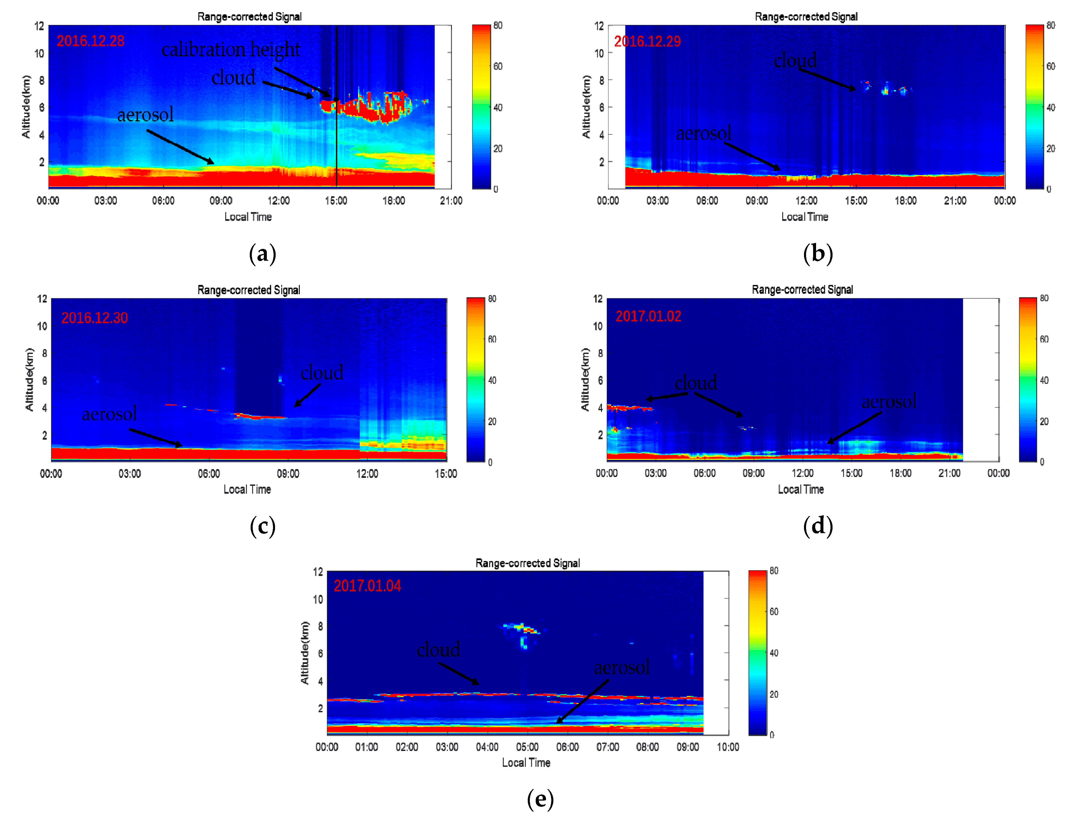
• The cloud LIDAR ratio is solved. The clean point after passing through the cloud layer is the iteration starting point A, and the cloud bottom height is the iterative end point B. It is assumed that there are few aerosol particles at this height; that is, the backscatter from point A to point B is mainly derived from clouds. When the thickness of the cloud is not large, the LIDAR energy can penetrate the cloud. At this time, the signal-to-noise ratio is sufficient, and the reference point can be selected above the cloud. Since the LIDAR ratio of cloud may be lower than that of aerosol, the extinction coefficient under cloud is generally smaller after the first inversion. The LIDAR ratio of low-altitude cloud between point A and point B is obtained by using the relationship between the extinction coefficient and backscatter ratio. Here, the condition for the end of the iteration is:

  $${\alpha }_a\left(z_B\right)\ge 1.01$$

  (4)
  When the extinction coefficient value of point B satisfies the Equation (4), the iteration ends, and the corresponding LIDAR ratio is the LIDAR ratio of cloud. Taking 15:00 in Figure 2a as an example, the values of cloud LIDAR ratio is 31.57 Sr. The LIDAR ratio of cloud in this study is 22.57–34.14 Sr.
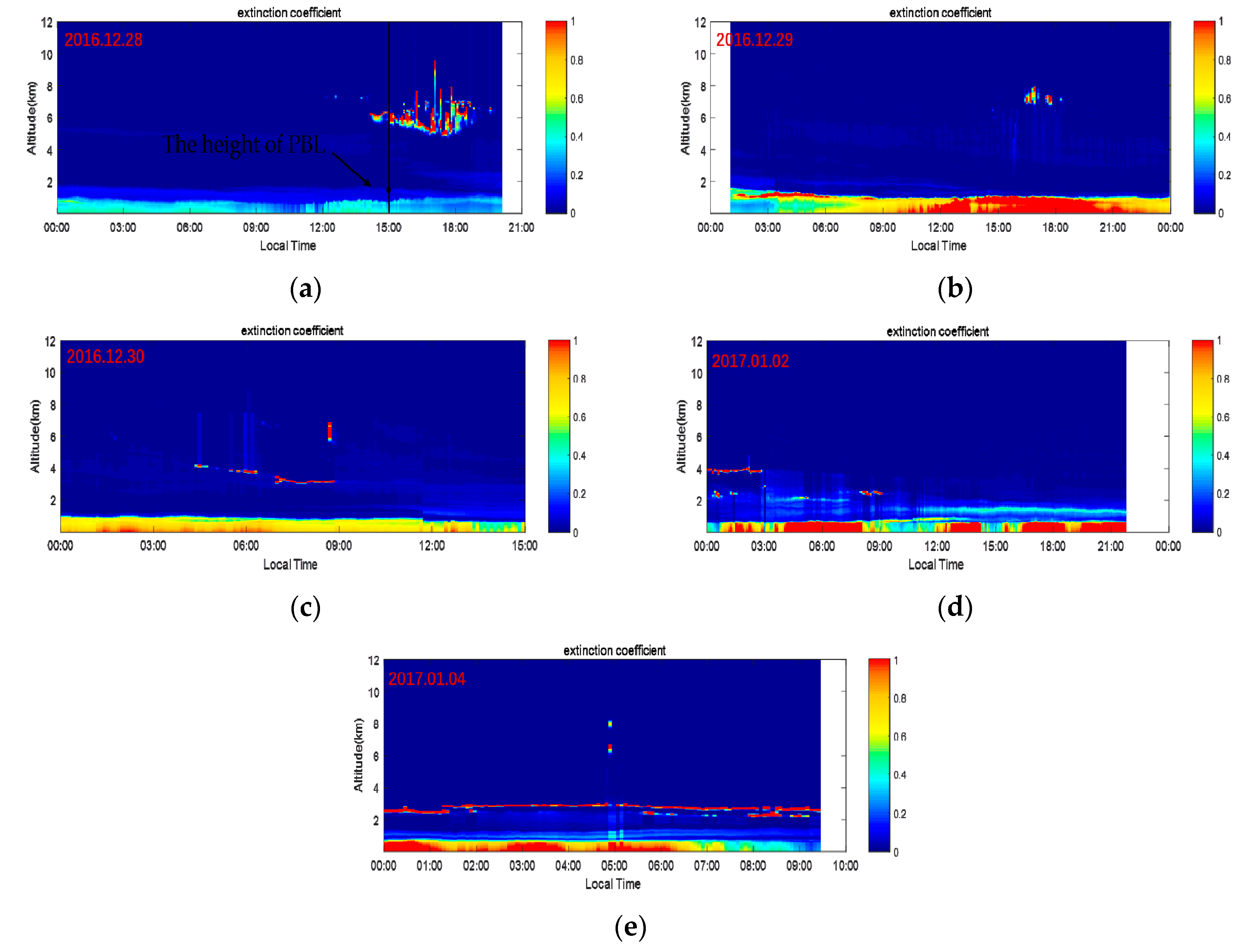
• The extinction coefficient profile below cloud is solved. According to the iterated aerosol extinction coefficient profile and changing LIDAR ratio, the extinction coefficient profile from near the ground to point B is obtained. When the all-weather extinction coefficient profile is obtained, the boundary layer properties of the atmosphere can be studied, and the aerosol optical depth (AOD) can be used to characterize the quality of the atmosphere. AOD is the integral of the extinction coefficient over a distance. The expression is

  $$AOD={\displaystyle \underset{z_1}{\overset{z_2}{\int }}\alpha (z)}dz,$$

  (5)

  where, $z_1$ represents the LIDAR return signal starting height; $z_2$ represents the height of the planetary boundary layer (PBL).

3. Results and Discussion

From 26 December 2016 to 5 January 2017, Huainan region experienced an 11-day period of alternations of hazy-foggy weather, which finally disappeared. The near-surface air quality experienced a change of “good–light pollution–moderate pollution–heavy pollution–good”. The source of the air quality index (AQI) is provided by China National Environmental Monitoring Centre. In this pollution incident, on December 26, the AQI reached 52. It then reached 140 on December 27, rose to 179 on December 29, and continued to rise over the following four days. It peaked at 250 on January 2, remained heavily polluted on January 3 and 4, and dropped to 72 on January 5, with a good air quality. The foggy-hazy composite pollutions were observed by VIIRS Suomi NPP from 27 December 2016 to 3 January 2017. Figure 3 shows the 1 km true-color images. As can be seen from the picture, On January 20, 2017, the AQI value was 74, and the air quality was good. The satellites were used to clearly see the ground. While during the pollution period, visibility is low in Huainan and its surrounding areas. In order to analyze the local hazy-foggy alternations caused by pollutants, firstly, the correlation analysis was conducted according to the concentration of particulate matter and other pollutants, and then, the influence of meteorological factors on the concentration of particulate matter was analyzed. Finally, the optical characteristics of aerosol particles in the foggy-hazy alternations were studied.

3.1. Analysis of the Meteorological Condition and Pollutant Concentrations

In order to further analyze the relationship between the particle concentration and polluted gas in the process of hazy-foggy composite pollution, this paper analyzes the data by time series plotting, as shown in Figure 4.

Among the results, PM₁₀ and PM_2.5 have a good synchronicity. The hourly average change of PM₁₀ is from 32 μg/m³ to 412 μg/m³, and the hourly average change of PM_2.5 is from 14 μg/m³ to 258 μg/m³. When the humidity rises, dry hygroscopic aerosol particles will grow [37]. The observation in north China shows that the particle size of aerosol particles will increase by 20–60% after water deposition [38], resulting in a "false high" of the PM_2.5 concentration when the relative humidity is high. According to Figure 4b, PM₁₀ concentrations are smaller than PM_2.5 concentrations at 4:00–13:00 on January 5, and the relative humidity at this time is 99%. This is not only the contribution of because of aerosol particles, but also because of the influence of relative humidity at this time. The relative humidity affects the measurement accuracy of the instrument, making the error larger. NO₂ and O₃ are negatively correlated. O₃ shows single-peak diurnal variation, which is a photochemical conversion characteristic. The changes of gaseous pollutants SO₂, NO₂, and particulate matter are also relatively consistent, and the peak change time of the three substances is basically the same, indicating that foggy-hazy weather has a relationship with gaseous precursors. This is because SO₂ and NO₂ are gaseous precursors of the secondary transformation of sulfate and nitrate in particulate matter, so the increase of concentration of SO₂ and NO₂ will also induce foggy-hazy pollution.

Figure 5 analyzes the relationship between four meteorological factors (relative humidity, temperature, wind speed, and visibility) and particulate matter. It can be seen from Figure 5a that the concentration of PM_2.5 is similar to the change trend of relative humidity, which is due to the fact that main inorganic salts on the particles, such as sulfate and nitrate, are highly hygroscopic substances. When the relative humidity in the environment is relatively high, the strong hygroscopic substance will absorb moisture and increase the particle size of the particles. Therefore, the probability of a heterogeneous reaction increases, resulting in increased pollution. It can be seen that a high humidity is more conducive to the formation of "secondary pollution" [39]. In this pollution incident, the daily average relative humidity is very high, and the relative humidity from December 28 to January 2 is between 70 and 80%, and the relative humidity in the rest of the weather is more than 85%. High-temperature weather is conducive to the dissipation of fog. When the temperature rises, the relative humidity decreases and the content of the fog in the air also decreases. In addition, particles with a poor thermal stability (such as ammonium nitrate) will evaporate into gases at high temperatures, so that the concentration of the solid particles is lowered [40]. However, the pollution occurred in winter. As can be seen from Figure 5b, the temperature range is 2–9 °C and the average temperature is only 4.6 °C. The surface wind speed affects the horizontal diffusion of air pollutants. When the wind speed is increased, the horizontal diffusion is accelerated and the pollutants are diffused and diluted quickly. When the wind speed decreases, the pollutants are easily enriched, resulting in increased pollution. It can be seen from Figure 5c that there is a strong negative correlation between the wind speed and PM_2.5 concentration. In the early stage of this weather process, the change of surface wind speed was not obvious, and the pollutant particles remained for a long time, providing a sufficient amount of time for secondary transformation. Moreover, due to the rapid development of the Yangtze River delta region, the urban buildings are more and more dense, resulting in an increase in the static wind state, which is even more detrimental to the horizontal diffusion of pollutants. Beginning on January 4, the wind speed gradually increased, peaking on January 5, and the pollutants gradually dissipated. According to the meteorological industry standard, when the visibility is less than 10.0 km, the weather phenomena, such as precipitation, dust, sand, floating dust, etc., are excluded, and the relative humidity is less than 80%, and it is classified as haze. Therefore, combined with the relationship between relative humidity, visibility, and particle concentration, the particle concentration on December 26 was not high, but the relative humidity was high and the visibility was low, indicating that the day was dominated by fog. From December 27 to January 1, the concentration of particulate matter was relatively high, and the relative humidity was less than 80%, indicating that haze was the dominant factor on these six days. From January 2 to January 4, the concentration of particulate matter continued to rise and the relative humidity was relatively high, which indicated that the fog and haze were alternately polluted on these three days.

When pollutants are released into the air, they are diluted and dispersed by turbulence. When the atmospheric environment is in a static state, the pollutants are not conducive to being diluted, and the inversion layer of "lower cold and upper warm" easily appears in the vertical direction. The inversion phenomenon is like a layer of "quilt", which blocks the vertical movement of air in the low air, and promotes the concentration of aerosol particles near the ground, resulting in the aggravation of haze pollution. Generally, in the early stage of pollution, inversion is often accompanied, which provides the previous conditions for the enrichment and transformation of pollutants. Figure 6 shows the vertical temperature profile measured by a radiosonde before and after haze at the meteorological station closet to the location of LIDAR. The results show that from December 27 to January 5, there is a strong inversion on the top of the haze layer and the colder surface, which is very different from that before the haze on December 26. During the process of foggy-hazy pollution, the height of the inversion layer is low. On the 27th and 29th, the height of the inversion layer was around 1000 m. The height of the inversion layer decreased from the 30th to 4th, when the average height was below 400 m, and the height of the inversion layer on the 5th was around 1500 m. The height of the inversion layer affects the vertical diffusion of pollutants, and the wind speed affects the horizontal diffusion, resulting in the accumulation of pollutants reaching the highest value on January 2 during the weather event, when the average wind speed was 0.875 m/s and the visibility was only 1.56 km.

In summary, from the relationship between the meteorological conditions and the concentration of pollutants, the meteorological conditions change little, and the concentration of particulate matter gradually increases. The weak surface wind speed, high relative humidity, low temperature, and strong inversion cause pollutants to gradually become enriched in the lower layer.

3.2. Aerosol Optical Properties during the Foggy-Hazy Weather

Since the Mie-LIDAR is a two-axis system, after a certain distance Z, the return signal can all enter the receiving field of view. At a distance of <Z, the backscattered light is partially accepted by the telescope. Therefore, experimental methods are often used to correct the overlap factor. First, we directed the LIDAR horizontally to emit a certain amount of laser pulses into the atmosphere. In the atmospheric return signal obtained at this time, since the atmospheric level is uniform, the atmospheric extinction coefficient and the backscattering coefficient were constant. We used the partial least squares fitting method to obtain the range-corrected signal, and obtained the overlap factor. Finally, we got the original return signal of 0–200 m.

Figure 7 shows 24-h backward trajectories during this weather process. An increase of the pollutant concentration occurred in three periods: (1) 9:00 on 27 December; (2) 15:00 on 29 December; and (3) 15:00 on 2 January. As can be seen from the figure, most of the air mass of 2000 m came from Inner Mongolia. Apart from January 2, most of the 500m and 1000 m air masses were raised in northern regions, such as Hebei and Shandong. The 500 m height of the air mass mostly came from surrounding cities in Huainan on January 2. Figure 7c shows the low-altitude air mass settled near to the ground at 6:00 on December 29 (local time). It can be seen that the near-surface air mass mainly came from the cities near the Huainan region and heavily polluted areas in the north, while the upper air mass came from Inner Mongolia.

Figure 8 shows the vertical profile of the extinction coefficient on December 28, 29, and 30 and January 2 and 4. Through LIDAR observation, the average height of PBL on December 28 is about 2km, but the height of PBL gradually declines after 29th. It is found that the falling movement of the lower troposphere causes the aerosol particles to gather in a very shallow layer, and the average height of the boundary layer is below 1000 m. During this period, the aerosol particles are mainly concentrated below 500 m, and the maximum aerosol load is concentrated around 100–300 m. The lower PBL and inversion layer limit the diffusion of pollutants in the vertical direction. On December 28, due to the low content of particulate matter, the average extinction coefficient was 0.37. After 16:00, since the height of PBL increased, the value AOD tended to increase. Starting from 01:00 on December 29, a layer of air mass with a high content of aerosol particles was observed, which tended to descend to the ground vertically. As a result, the accumulation number of aerosols on the ground increased after the 29th, which is consistent with the backward trajectories in Figure 7b,c. The air mass settled to the ground at approximately 6:00 local time on December 29. The average wind speed on the day was 2.25 m/s, and the horizontal diffusion was slow. The average temperature was 2 °C, and the continuous low temperature was not conducive to the formation of wind and the reduction of water vapor content in the air. The relative humidity was high, reaching the daily average of 78%, which further promoted the generation of "secondary pollution". All these meteorological factors are not conducive to the diffusion of pollutants, so the concentration of particulate matter and gaseous pollutants on the 29th increased compared with the previous three days, and the foggy-hazy weather continued and was aggravated after the 29th. On December 30, the average wind speed decreased to 1.5 m/s, and the relative humidity was 77%. The particulate matter content continued to rise, and the pollution weather continued. Until January 2, the average wind speed dropped to 0.875 m/s, PM_2.5 reached its maximum value of 258 μg/m³, and the average extinction coefficient was 0.76, indicating the most serious pollution. On January 4, there was rainfall according to the records of the Shouxian Meteorological Bureau. With the increase of wind speed and temperature, the horizontal diffusion speed of aerosol particles was accelerated. After 9:00, the amount of near-surface aerosol accumulation was significantly reduced. On January 5, the average wind speed reached 5.75 m/s, and pollutants were diluted and transported by the wind. The foggy-hazy weather ended and the visibility improved.

Figure 9 shows the relationship between the particulate matter and the AOD (using the algorithm proposed in Section 2.2 above). The blue line represents PM_2.5 and the pink line represents AOD. According to the extinction coefficient profile, since the foggy-hazy phenomenon was not very serious on December 28, the relationship between PM_2.5 and AOD was not significant. After 16:00, as the boundary layer tended to increase, AOD also increased. On the following days, the curve trends of PM_2.5 and AOD were roughly the same. The air mass settled on December 29, and the concentration of particles increased along with the static and stable weather, resulting in the values of PM_2.5 and AOD both increasing. This indicates that there is a positive correlation between PM_2.5 and AOD. Through correlation analysis, we found that R² = 0.7368, showing a linear relationship. After January 4, the haze began to weaken, and the AOD value showed a decreasing trend. On January 5, the AQI index recovered well, which was basically consistent with the change of the extinction coefficient, indicating that AOD could also reflect the condition of pollution. Yang et al. [41] investigated the relationship between PM_2.5 and AOD acquired by satellites at different temporal and regional scales. Our study investigated the relationship between PM_2.5 and the near-surface AOD obtained by LIDAR in the Huainan area, and the influence of the low-altitude cloud is removed when acquiring data.

Figure 10 shows the aerosol subtypes on December 30 and January 1. Since the observation of CALIPSO is global and large-scale, our research area selection range is Anhui Province. Through the vertical continuous detection of CALIPSO, we found that polluted dust-type aerosols are mainly concentrated in the middle and bottom layers of the atmospheric troposphere, and polluted continental-type aerosols are mainly concentrated in the bottom layer of the atmospheric troposphere. Among them, the polluted dust-type aerosol is thicker, and the thickness of this type of aerosol particles is close to 5 km. According to the analysis of HYSPLIT, the aerosol particles in the middle layer of the troposphere are transmitted to the Huainan area along with the air mass. The polluted continental-type aerosols concentrated in the bottom layer come from human activities.

Figure 11 shows the VIIRS deep blue AOD at 550 nm in Huainan. Due to the cloud cover, the AOD values of five days in this weather process were selected, and the AOD values showed obvious spatial gradient, which were larger in the north and smaller in the south of Huainan. The values of AOD over the Huainan area were 0.056, 0.504, 0.571, and 0.728. During the occurrence of foggy-hazy weather, the increasing AOD value represents an increasing amount of aerosol particle aggregation, which is basically consistent with the ground-based LIDAR observation. Figure 12 shows the VIIRS angstrom exponent (AE) at 550 nm in Huainan. The values of AE over the Huainan area were 1.481 and 1.30. It can be seen that on December 30 and 31, the pollutants are mainly fine-mode particles, indicating that the main pollutants are from man-made emissions. Due to the limited amount of AE data, it is not possible to judge whether the external air mass is mixed with the local man-made emissions, resulting in the change of the pollutant particle size.

Through the observation and analysis of the pollution weather in the Huainan area, it has been found that the data analysis of ground instruments and satellite sensor is consistent and reasonable in terms of the variation of the pollutant concentration and spatial distribution.

4. Conclusions

In this paper, the cooperative effects of ground-based LIDAR and satellite sensors were used to observe the weather conditions in the Huainan region, where continuous foggy-hazy alternations occurred from December 26, 2016 to January 5, 2017. This study explored the course of the event by examining pollutant concentrations, meteorological factors, and aerosol optical properties, resulting in the following observations:

• Extinction coefficient inversion in low-altitude cloud weather: Under the condition of low altitude cloud, the extinction coefficient of cloud particles for LIDAR signals is different from that of aerosol particles, which leads to small extinction coefficient results when Fernald inversion is used, meaning that accurate inversion extinction coefficients have certain limitations. In this paper, segmentation inversion is used, and the backscatter ratio is used to identify the low-altitude cloud clouds. Then, the differential zero-crossing method is used to identify the cloud top height and the cloud bottom height, and the cloud LIDAR ratio is reasonably selected through iterative inversion. Accurate inversion of the extinction coefficient profile is realized in this paper, and the LIDAR ratio of cloud in this period is 22.57–34.14 Sr.
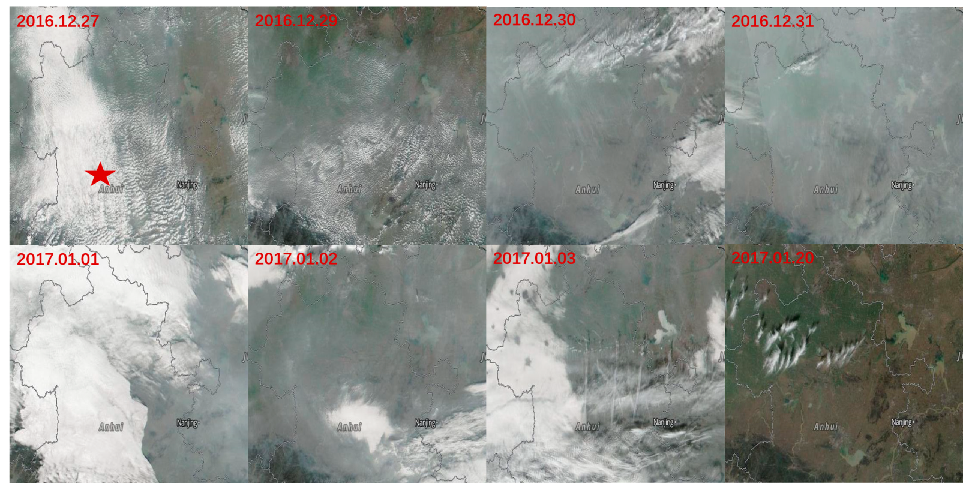
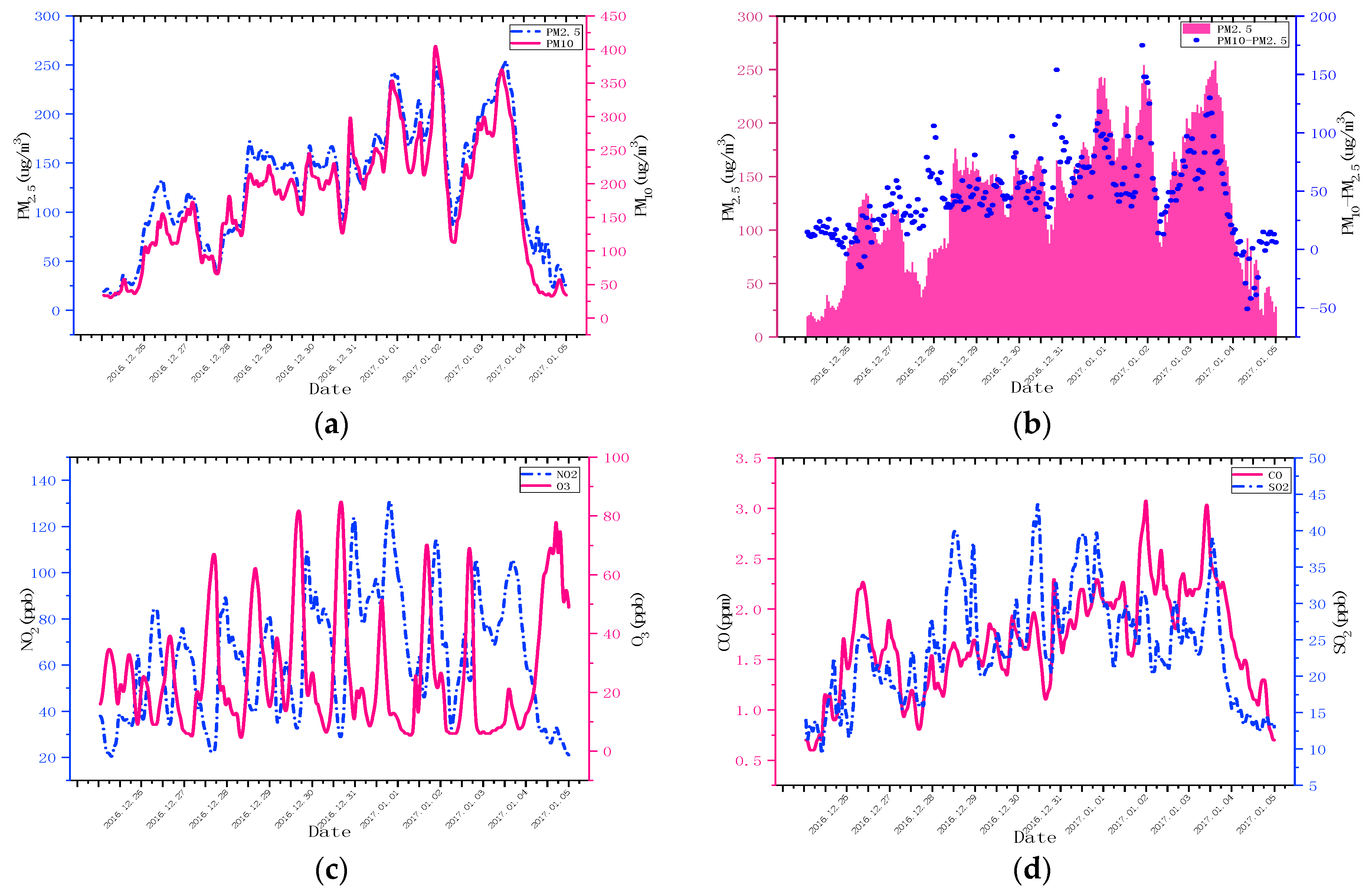
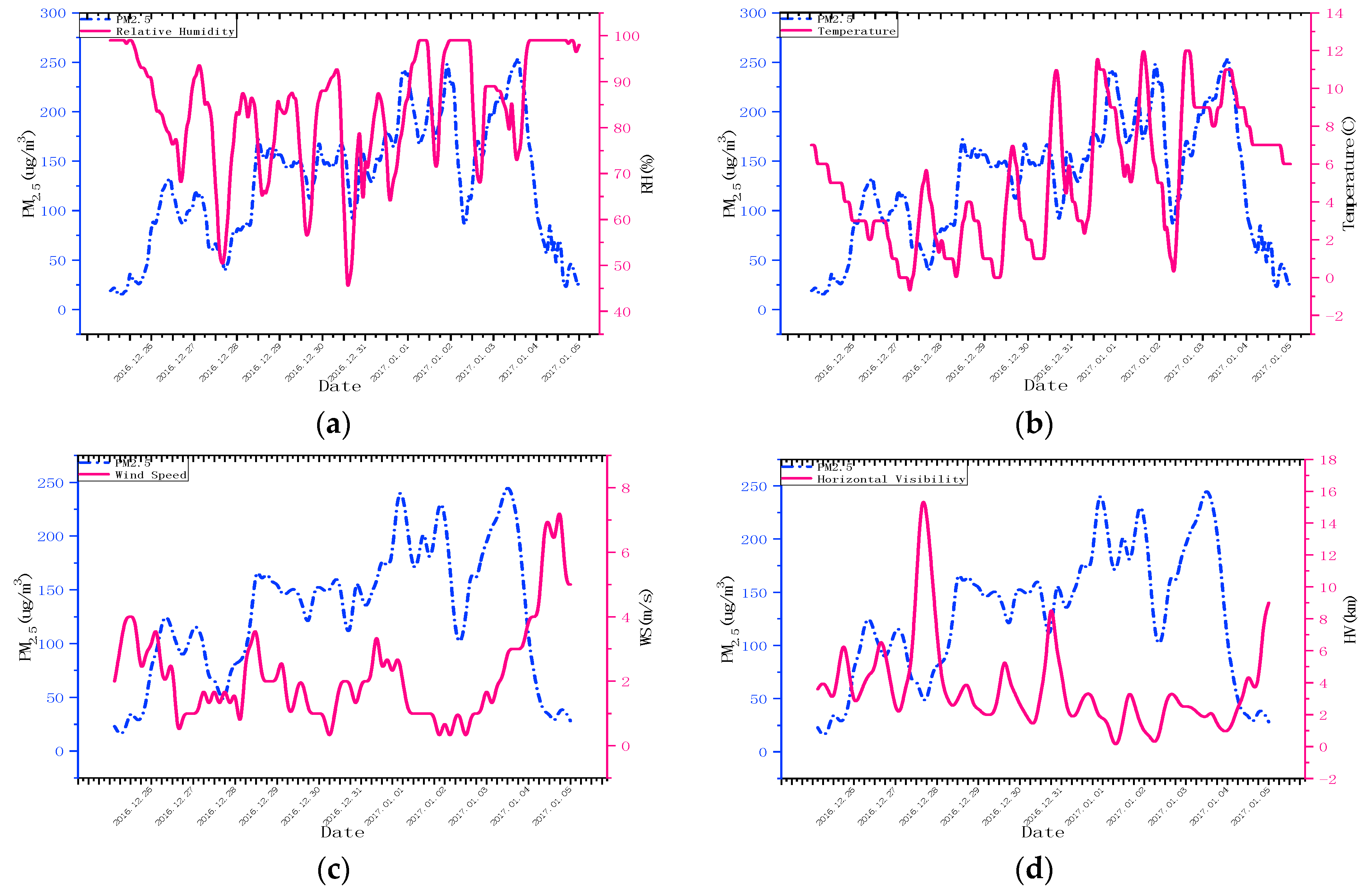
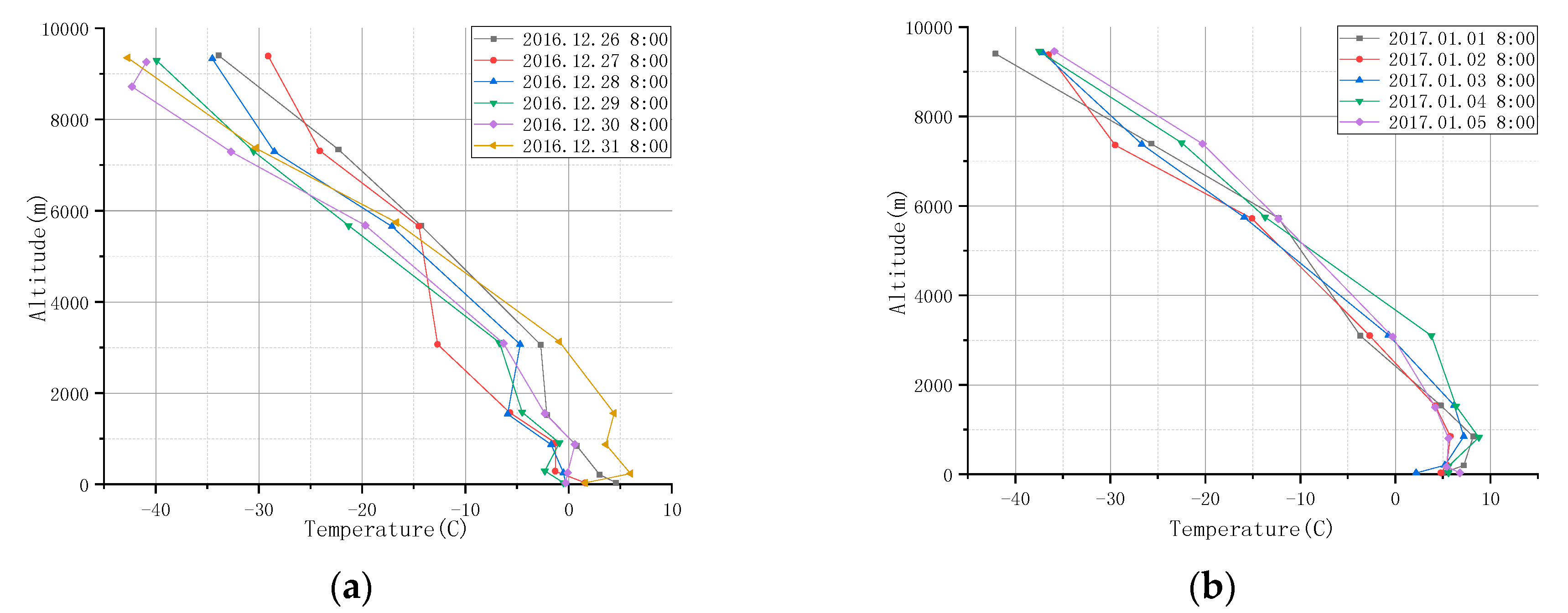
• Analysis of the meteorological condition and pollutant concentrations: During the formation of this weather, PM_2.5 and major trace gases increased significantly, the photochemical reaction and heterogeneous reaction process may have led to the increase of sulfate and nitrate, and the influence of humidity led to the formation of "secondary pollution", meaning that this event had a greater impact on the region. A weak surface wind speed, high relative humidity, low temperature, and strong inversion caused pollutants to gradually become enriched in the lower layer. The accumulation of pollutants caused the continuous formation of haze after December 29, resulting in visibility in the Huainan area below 10 km.
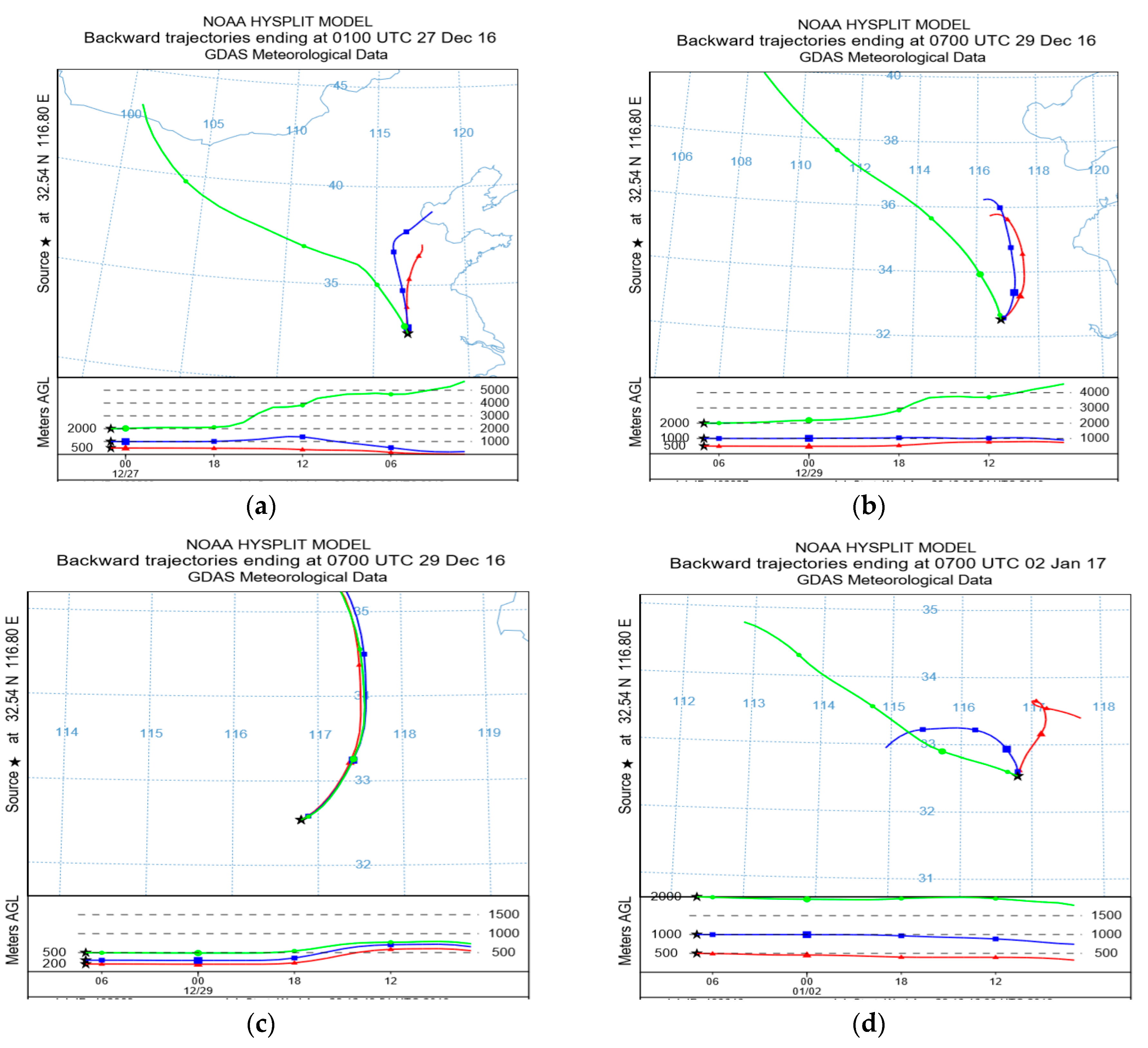
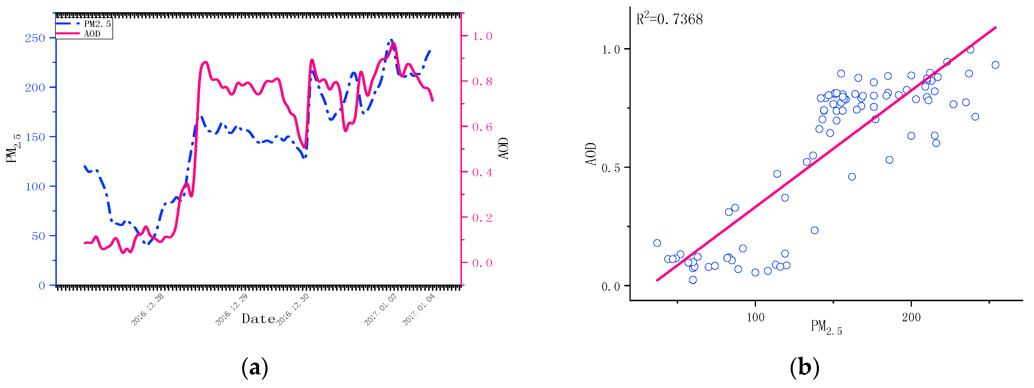
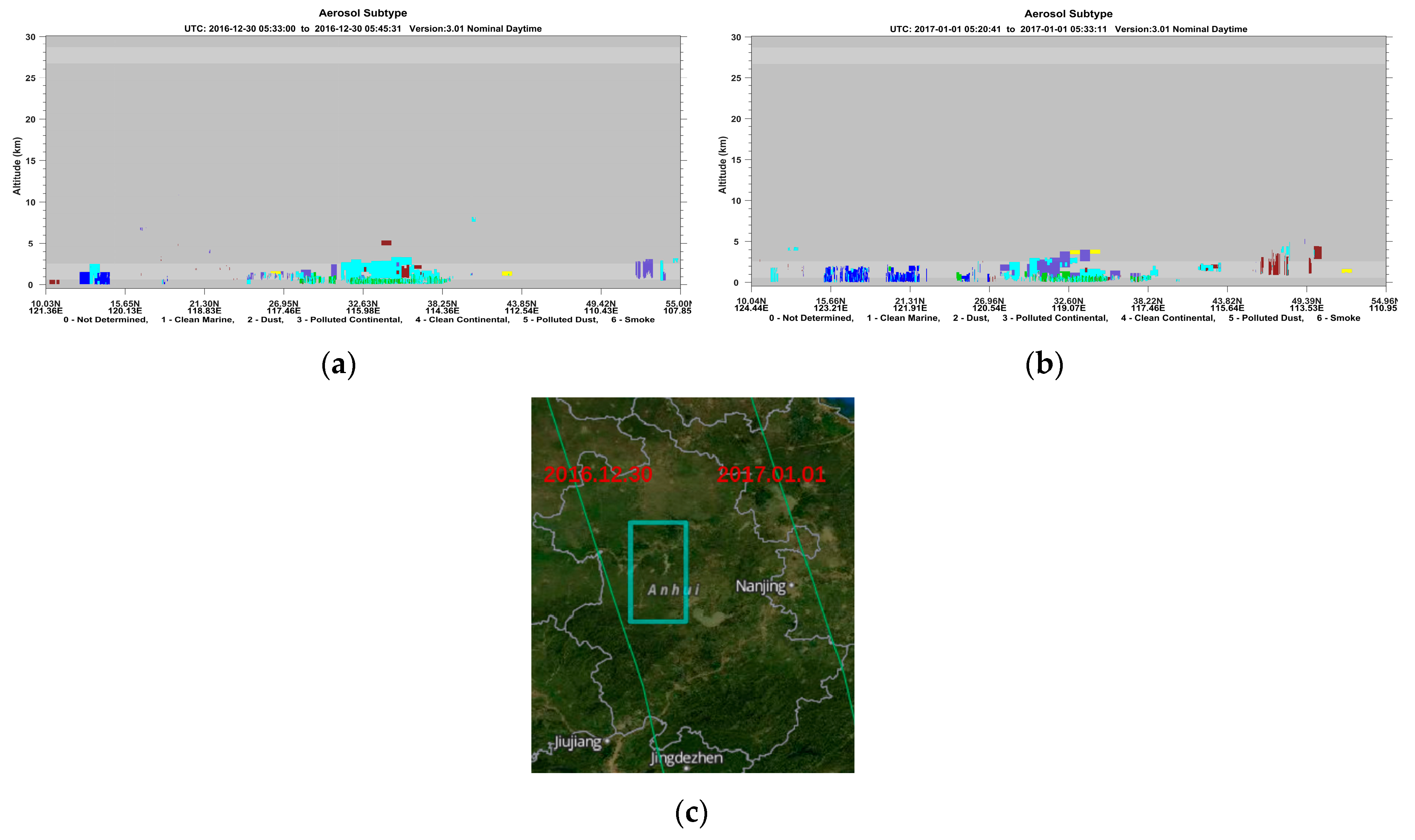
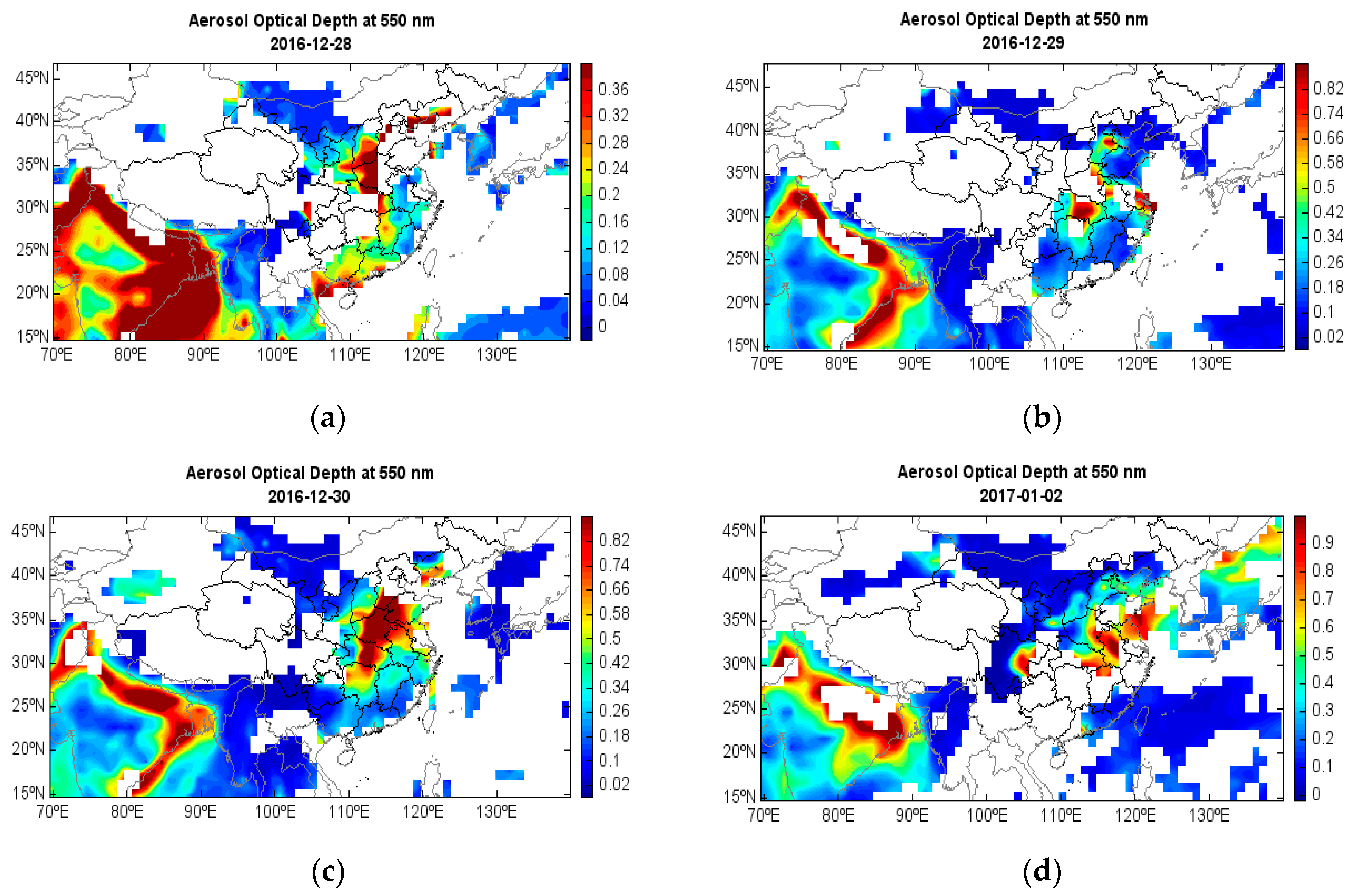
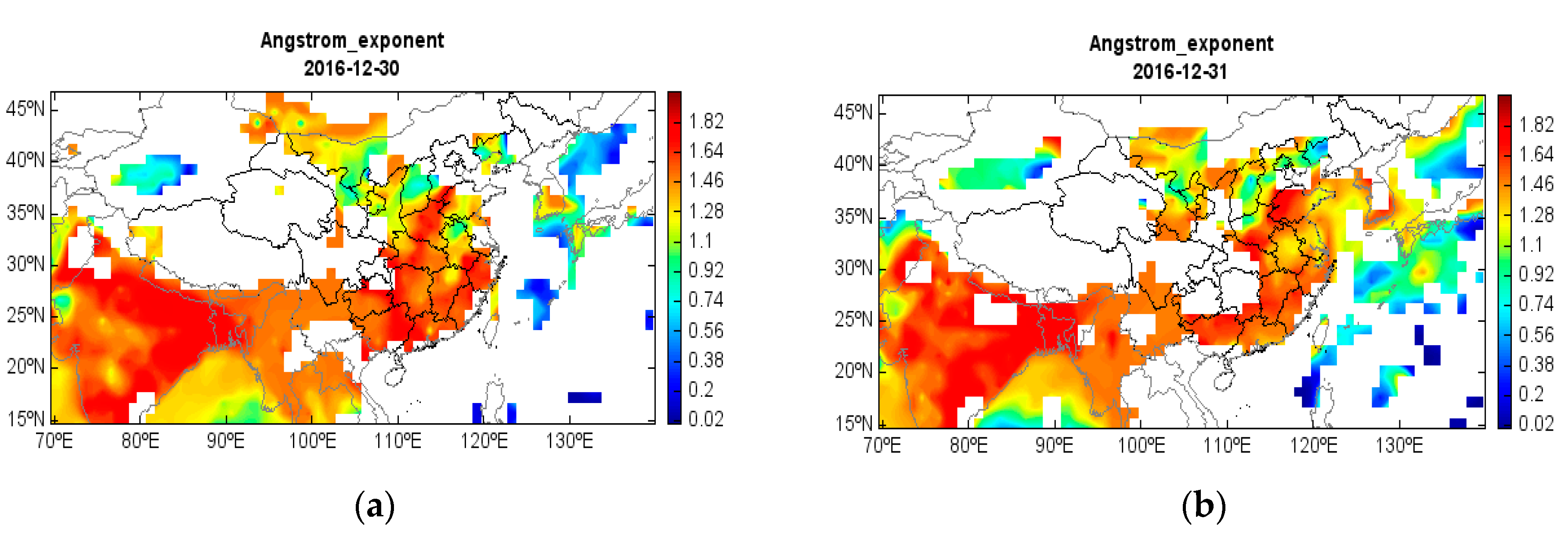
• Aerosol optical properties: In this case, the near-surface air mass mainly came from the cities near the Huainan region and the heavily polluted areas in the north, while the upper air mass came from Inner Mongolia. Through the inversion of the extinction coefficient profile of ground-based LIDAR data, with the settlement of pollutant air mass on December 29, meteorological factors acted as incentives, causing pollutants to gradually become enriched. After January 4, there was a gradual easing trend. The correlation index of PM_2.5 and AOD was 0.7368, indicating that there is a definite linear relationship between them, and AOD can also reflect the pollution condition of this region. The AOD calculated by the ground-based LIDAR is consistent with the AOD trend obtained by the spaceborne sensor, and the AOD value peaks on January 2.

The analysis of the weather process in this paper can provide a research basis for foggy-hazy pollution in the Huainan region. In future studies, we will further calculate the cloud LIDAR ratio under the influence of multiple scattering, and compare the aerosol optical characteristics in different seasons and regions with the long-term observation data, so as to improve our understanding of the impact of the atmospheric environment.

References

1. Zhang, M.; Ma, Y.; Gong, W.; Zhu, Z. Aerosol Optical Properties of a Haze Episode in Wuhan Based on Ground-Based and Satellite Observations. Atmosphere 2014, 5, 699–719. [Google Scholar] [CrossRef] [Green Version]
2. Christodoulakis, J.; Varotsos, C.A.; Cracknell, A.P.; Kouremadas, G.A. The deterioration of materials as a result of air pollution as derived from satellite and ground based observations. Atmos. Environ. 2018, 185, 91–99. [Google Scholar] [CrossRef] [Green Version]
3. Kulmala, M.; Lappalainen, H.K.; Petäjä, T.; Kurten, T.; Kerminen, V.M.; Viisanen, Y.; Hari, P.; Sorvari, S.; Bäck, J.; Bondur, V.; et al. Introduction: The Pan-Eurasian Experiment (PEEX)—Multidisciplinary, multiscale and multicomponent research and capacity-building initiative. Atmos. Chem. Phys. 2015, 15, 13085–13096. [Google Scholar] [CrossRef]
4. Nie, W.; Ding, A.J.; Xie, Y.N.; Xu, Z.; Mao, H.; Kerminen, V.M.; Zheng, L.F.; Qi, X.M.; Huang, X.; Yang, X.Q.; et al. Influence of biomass burning plumes on HONO chemistry in eastern China. Atmos. Chem. Phys. 2015, 15, 1147–1159. [Google Scholar] [CrossRef] [Green Version]
5. Gui, K.; Che, H.; Chen, Q.; An, L.; Zeng, Z.; Guo, Z.; Zheng, Y.; Wang, H.; Wang, Y.; Yu, J.; et al. Aerosol Optical Properties Based on Ground and Satellite Retrievals during a Serious Haze Episode in December 2015 over Beijing. Atmosphere 2016, 7, 70. [Google Scholar] [CrossRef]
6. Che, H.; Zhao, H.; Wu, Y.; Xia, X.; Zhu, J.; Wang, H.; Wang, Y.; Sun, J.; Yu, J.; Zhang, X.; et al. Analyses of aerosol optical properties and direct radiative forcing over urban and industrial regions in Northeast China. Meteorol. Atmos. Phys. 2015, 127, 345–354. [Google Scholar] [CrossRef]
7. Lee, K.H.; Kim, Y.J.; Kim, M.J. Characteristics of aerosol observed during two severe haze events over Korea in June and October 2004. Atmos. Environ. 2006, 40, 5146–5155. [Google Scholar] [CrossRef]
8. Qin, K.; Wu, L.; Wong, M.S.; Letu, H.; Hu, M.; Lang, H.; Sheng, S.; Teng, J.; Xiao, X.; Yuan, L. Trans-boundary aerosol transport during a winter haze episode in China revealed by ground-based Lidar and CALIPSO satellite. Atmos. Environ. 2016, 141, 20–29. [Google Scholar] [CrossRef] [Green Version]
9. Liu, B.; Ma, Y.; Gong, W.; Zhang, M.; Yang, J. Study of continuous air pollution in winter over Wuhan based on ground-based and satellite observations. Atmos. Pollut. Res. 2018, 9, 156–165. [Google Scholar] [CrossRef]
10. Tao, W.K.; Chen, J.P.; Li, Z.; Wang, C.; Zhang, C. Impact of Aerosols on Convective Clouds and Precipitation. Rev. Geophys. 2012, 50. [Google Scholar] [CrossRef]
11. Hansen, J.; Sato, M.; Ruedy, R.; Lacis, A.; Oinas, V. Global warming in the twenty-first century: An alternative scenario. Proc. Natl. Acad. Sci. USA 2000, 97, 9875–9880. [Google Scholar] [CrossRef] [PubMed] [Green Version]
12. Peng, S.; Zhou, S.; Wang, M.; Chen, S.; Chen, A. Characteristics of a Continuous Fog and Haze Weather in Nanjing and Its Causes. J. Arid Meteorol. 2018, 36, 282–289. [Google Scholar] [CrossRef]
13. Zhou, X.; Ni, C.; Tan, G. Characteristics and Cause Analysis of a Persistent Haze Process in Southern Sichuan Basin. Plateau Mt. Meteorol. Res. 2018, 38, 53–57. [Google Scholar] [CrossRef]
14. Pan, L.; Li, P.; Yu, L. Causes and Forecast Analysis of Fog and Haze in Yancheng. J. Agric. Catastrophology 2018, 8, 52–53. [Google Scholar] [CrossRef]
15. Yang, Z. The cause of haze and related environmental remediation measures. Environ. Dev. 2018, 30, 242–244. [Google Scholar] [CrossRef]
16. Wang, Y.; Zhuang, G.; Sun, Y.; An, Z. The variation of characteristics and formation mechanisms of aerosols in dust, haze, and clear days in Beijing. Atmos. Environ. 2006, 40, 6579–6591. [Google Scholar] [CrossRef]
17. Gong, H.; Wu, N.; Ni, Y.; Chen, W.; Lu, J.; Chen, X.; Lv, Y.; Zhang, W.; Li, Z.; Xu, H.; et al. Comparison between dust and haze aerosol properties of the 2015 Spring in Beijing using ground-based sun photometer and LIDAR. In AOPC 2015: Optical and Optoelectronic Sensing and Imaging Technology; SPIE: Bellingham, WA, USA, 2015. [Google Scholar] [CrossRef]
18. Yang, Y.R.; Liu, X.G.; Qu, Y.; An, J.L.; Jiang, R.; Zhang, Y.H.; Sun, Y.L.; Wu, Z.J.; Zhang, F.; Xu, W.Q.; et al. Characteristics and formation mechanism of continuous hazes in China: A case study during the autumn of 2014 in the North China Plain. Atmos. Chem. Phys. 2015, 15, 8165–8178. [Google Scholar] [CrossRef]
19. Tao, M.; Chen, L.; Wang, Z.; Tao, J.; Su, L. Satellite observation of abnormal yellow haze clouds over East China during summer agricultural burning season. Atmos. Environ. 2013, 79, 632–640. [Google Scholar] [CrossRef]
20. Tao, M.; Chen, L.; Wang, Z.; Ma, P.; Tao, J.; Jia, S. A study of urban pollution and haze clouds over northern China during the dusty season based on satellite and surface observations. Atmos. Environ. 2014, 82, 183–192. [Google Scholar] [CrossRef]
21. Lin, J.C.; Matsui, T.; Pielke, R.A.; Kummerow, C. Effects of biomass-burning-derived aerosols on precipitation and clouds in the Amazon Basin: A satellite-based empirical study. J. Geophys. Res. 2006, 111. [Google Scholar] [CrossRef]
22. Huang, X.; Ding, A.; Liu, L.; Liu, Q.; Ding, K.; Niu, X.; Nie, W.; Xu, Z.; Chi, X.; Wang, M.; et al. Effects of aerosol–radiation interaction on precipitation during biomass-burning season in East China. Atmos. Chem. Phys. 2016, 16, 10063–10082. [Google Scholar] [CrossRef]
23. Liu, X.G.; Li, J.; Qu, Y.; Han, T.; Hou, L.; Gu, J.; Chen, C.; Yang, Y.; Liu, X.; Yang, T.; et al. Formation and evolution mechanism of regional haze: A case study in the megacity Beijing, China. Atmos. Chem. Phys. 2013, 13, 4501–4514. [Google Scholar] [CrossRef]
24. Xie, C.; Nishizawa, T.; Sugimoto, N.; Matsui, I.; Wang, Z. Characteristics of aerosol optical properties in pollution and Asian dust episodes over Beijing, China. Appl. Opt. 2008, 47, 4945–4951. [Google Scholar] [CrossRef] [PubMed]
25. Tian, Z.; Xie, H.; Bi, J.; Huang, Z.; Huang, J.; Shi, J.; Zhang, B.; Wu, Z.J.A. Lidar Measurements of Dust Aerosols during Three Field Campaigns in 2010, 2011 and 2012 over Northwestern China. Atmosphere 2018, 9, 173. [Google Scholar] [CrossRef]
26. Wei, G.; Zhang, S.; Ma, Y.J.A. Aerosol Optical Properties and Determination of Aerosol Size Distribution in Wuhan, China. Atmosphere 2014, 5, 81–91. [Google Scholar] [CrossRef] [Green Version]
27. Xin, J.; Wang, Y.; Li, Z.; Wang, P.; Hao, W.M.; Nordgren, B.L.; Wang, S.; Liu, G.; Wang, L.; Wen, T.; et al. Aerosol optical depth (AOD) and Ångström exponent of aerosols observed by the Chinese Sun Hazemeter Network from August 2004 to September 2005. J. Geophys. Res. 2007, 112. [Google Scholar] [CrossRef]
28. Lang, X.; Kebiao, M.; Zhiwen, S.; Ying, M. Introduction of Suomi NPP VIIRS and Its Application on Cloud Detection. Adv. Geosci. 2013, 3, 271–276. [Google Scholar] [CrossRef]
29. Liu, Z.; Liu, D.; Huang, J.; Vaughan, M.; Uno, I.; Sugimoto, N.; Kittaka, C.; Trepte, C.; Wang, Z.; Hostetler, C. Airborne dust distributions over the Tibetan Plateau and surrounding areas derived from the first year of CALIPSO LIDAR observations. Atmos. Chem. Phys. 2008, 8, 5045–5060. [Google Scholar] [CrossRef]
30. Winker, D.M.; Vaughan, M.A.; Omar, A.; Hu, Y.; Powell, K.A.; Liu, Z.; Hunt, W.H.; Young, S.A. Overview of the CALIPSO mission and CALIOP data processing algorithms. J. Atmos. Ocean. Technol. 2009, 26, 2310–2323. [Google Scholar] [CrossRef]
31. Stein, A.F.; Draxler, R.R.; Rolph, G.D.; Stunder, B.J.B.; Ngan, F. NOAA’s HYSPLIT atmospheric transport and dispersion modeling system. Bull. Am. Meteorol. Soc. 2016, 96, 2059–2077. [Google Scholar] [CrossRef]
32. Fernald, F.G.; Herman, B.M.; Reagan, J.A. Determination of Aerosol Height Distributions by Lidar. J. Appl. Meteorol. 1972, 11, 482–489. [Google Scholar] [CrossRef] [Green Version]
33. Burton, S.P.; Ferrare, R.A.; Hostetler, C.A.; Hair, J.W. Aerosol classification using airborne High Spectral Resolution Lidar measurements—Methodology and examples. Atmos. Meas. Tech. Discuss. 2011, 4, 73–98. [Google Scholar] [CrossRef]
34. Damien, J.; Raymond, R.; Jacques, P.; Yongxiang, H.; Zhaoyan, L.; Ali, O.; Peng-Wang, Z. CALIPSO LIDAR ratio retrieval over the ocean. Opt. Express 2011, 19, 18696. [Google Scholar] [CrossRef]
35. Su, J.; Liu, Z.; Wu, Y.; McCormick, M.P.; Lei, L. Retrieval of multi-wavelength aerosol LIDAR ratio profiles using Raman scattering and Mie backscattering signals. Atmos. Environ. 2013, 79, 36–40. [Google Scholar] [CrossRef]
36. Müller, D.; Ansmann, A.; Mattis, I.; Tesche, M.; Wandinger, U.; Althausen, D.; Pisani, G. Aerosol-type-dependent LIDAR ratios observed with Raman LIDAR. J. Geophys. Res. 2007, 112. [Google Scholar] [CrossRef]
37. Shi, Y.; Ge, M.; Wang, W. Hygroscopicity of internally mixed aerosol particles containing benzoic acid and inorganic salts. Atmos. Environ. 2012, 60, 9–17. [Google Scholar] [CrossRef]
38. Pan, X.L.; Yan, P.; Tang, J.; Ma, J.Z.; Wang, Z.F.; Gbaguidi, A.; Sun, Y.L. Observational study of influence of aerosol hygroscopic growth on scattering coefficient over rural area near Beijing mega-city. Atmos. Chem. Phys. 2009, 9, 7519–7530. [Google Scholar] [CrossRef] [Green Version]
39. Lin, Z.J.; Tao, J.; Chai, F.H.; Fan, S.J.; Yue, J.H.; Zhu, L.H.; Ho, K.F.; Zhang, R.J. Impact of relative humidity and particles number size distribution on aerosol light extinction in the urban area of Guangzhou. Atmos. Chem. Phys. 2013, 13, 1115–1128. [Google Scholar] [CrossRef] [Green Version]
40. Zhao, X.J.; Zhao, P.S.; Xu, J.; Meng, W.; Pu, W.W.; Dong, F.; He, D.; Shi, Q.F. Analysis of a winter regional haze event and its formation mechanism in the North China Plain. Atmos. Chem. Phys. 2013, 13, 5685–5696. [Google Scholar] [CrossRef] [Green Version]
41. Yang, Q.; Yuan, Q.; Yue, L.; Li, T.; Zhang, L. The relationships between PM2.5 and AOD in China: About and behind spatiotemporal variations. Environ. Pollut. 2018, 248, 526–535. [Google Scholar] [CrossRef]
Figure 1. The geographical location of Huainan. The red area represents Huainan in Anhui Province.
Atmosphere 10 00656 g001
Figure 2. Vertical profile of range-corrected signal: (a) December 28 00:00–20:00; (b) December 29, 01:05–23:55; (c) December 30 00:00–10:40 and 11:00–14:55; (d) January 2 00:00–22:00; (e) January 4 00:00–9:20.
Atmosphere 10 00656 g002
Figure 3. The Visible Infrared Imaging Radiometer Suite (VIIRS) Suomi National Polar-orbiting Partnership (NPP) 1 km true-color images during the foggy-hazy composite pollutions and a sunny day.
Atmosphere 10 00656 g003
Figure 4. Concentrations of PM2.5, PM10, SO2, CO, and NO2 in Huainan.
Atmosphere 10 00656 g004
Figure 5. Variations of PM2.5 concentration with meteorological parameters: (a) Relative humidity; (b) temperature; (c) wind speed; (d) horizontal visibility.
Atmosphere 10 00656 g005
Figure 6. The vertical temperature profile: (a) December 26, 2016 to December 31, 2016; (b) January 1, 2017 to January 5, 2017.
Atmosphere 10 00656 g006
Figure 7. 24-h backward trajectories: (a) 9:00 on 27 December (local time); (b) 15:00 on 29 December (local time); (c) 15:00 on 29 December (local time); (d) 15:00 on 2 January (local time).
Atmosphere 10 00656 g007
Figure 8. Vertical profile of particle extinction: (a) December 28 00:00–20:00; (b) December 29, 01:05–23:55; (c) December 30 00:00–10:40 and 11:00–14:55; (d) January 2 00:00–22:00; (e) January 4 00:00–9:20.
Atmosphere 10 00656 g008
Figure 9. Relationship between particulate matter and the aerosol optical depth (AOD): (a) Variation in AOD and the concentration of particulate matter; (b) correlation between the concentration of particulate matter and AOD.
Atmosphere 10 00656 g009
Figure 10. The vertical continuous detection of CALIPSO: (a) Aerosol subtype on December 30; (b) aerosol subtype on January 1; (c) the CALIPSO orbits with green lines and the Huainan region with a blue box.
Atmosphere 10 00656 g010
Figure 11. VIIRS deep blue AOD at 550 nm in Huainan.
Atmosphere 10 00656 g011
Figure 12. VIIRS Angstrom exponent at 550 nm in Huainan.
Atmosphere 10 00656 g012