Abstract
In the present work, dry temperature profiles provided by the Constellation Observing System for Meteorology, Ionosphere, and Climate (COSMIC) radio occultation (RO) mission and the horizontal wind field provided by the European Centre for Medium-Range Weather Forecasts (ECMWF) reanalysis are combined for the first time to retrieve the magnitudes of gravity wave (GW) pseudomomentum flux (PMF). The vertical wave parameters, including Brunt–Väisälä frequencies, potential energy (Ep), and vertical wavelengths, are retrieved from RO temperature profiles. The intrinsic frequencies, which are retrieved from the horizontal wind field of ERA-Interim, are combined with the vertical wave parameters to derive the horizontal wavelengths and magnitudes of the PMF of GWs. The feasibility of this new strategy is validated first by comparing the distributions of GW parameters during June, July, and August (JJA) 2006 derived this way with those derived by previous studies. Then the seasonal and interannual variations of the distributions of GW PMF for three altitude ranges, 20–25 km, 25–30 km, and 30–35 km, over the globe during the seven years from June 2006 to May 2013 are presented. It is shown that the three altitude intervals share similar seasonal and interannual distribution patterns of GW PMF, while the magnitudes of GW PMF decrease with increased height and the hot spots of GW activity are the most discernable at the lowest altitude interval of 20–25 km. The maximums of PMF usually occur at latitudes around 60° in the winter hemispheres, where eastward winds prevail, and the second maximums exist over the subtropics of the summer hemispheres, where deep convection occurs. In addition, the influence of quasi-biennial oscillation (QBO) on both GW PMF and zonal winds is discernible over subtropical regions. The present work complements the GW PMF interannual variation patterns derived based on satellite observations by previous studies in terms of the altitude range, latitude coverage, and time period analyzed.
1. Introduction
It is well known that gravity waves (GWs) play an important role in middle-atmospheric circulation by transporting energy and momentum in their vertical or horizontal propagations [1,2], and GW parameterizations form a key component of climate and weather models [3,4]. Among all the parameters that characterize GW activities, the vertical flux of horizontal momentum, or simply momentum flux (MF), is the most prominent, because it is crucial for estimating the level of wave breaking and hence the effect of GWs on mean flow [5,6].
GW activities have been studied with observations from radiosonde [7,8], radar [9], rocket soundings [10], lidar [11], and limb- and nadir-scanning satellites [12,13]. In recent years, the Global Positioning System (GPS) radio occultation (RO) technique has drawn much attention in GW-related studies. Compared with measurements from other traditional techniques, the large amount of temperature profiles provided by GPS RO missions, which have high precision, high vertical resolution, global coverage, and long-term stability, enable a thorough understanding of the mesoscale perturbations caused by GWs over the globe [10,14].
Some GW parameters can be deduced from single RO temperature profiles, such as temperature perturbations, vertical wavelengths, and potential energy (Ep). The global distributions of GW potential energy have been investigated based on data from different RO missions including GPS/Meteorology (GPS/MET) [15], Challenging Minisatellite Payload (CHAMP) [16,17], Constellation Observing System for Meteorology, Ionosphere, and Climate (COSMIC) [18,19], and MetOp [20]. The Ep values derived from RO temperature profiles were validated with reference to those derived from model data [20] and from radiosonde observations [21]. The latitudinal variations of RO-derived vertical wavenumber spectra of GWs were studied, and evidence of the interaction between vertically propagating convectively generated GWs and background mean flow were demonstrated [16,22]. Using RO temperature profiles, spatial and temporal variations of Ep values during stratospheric sudden warmings (SSWs) were investigated [23,24], and the relationship between GW Ep and tropopause height was discussed [25,26].
Unlike GW Ep, which can be derived directly from temperature perturbations, retrieving GW MF requires both vertical and horizontal information of GWs, and the horizontal wave parameters cannot be derived from single RO temperature profiles. The horizontal wave parameters of GWs are traditionally derived based on wind data [7,8], which is not directly available from RO products. Ern et al. [2] presented a method to derive MF using pairs of neighboring temperature perturbation profiles and applied it first to satellite data from Cryogenic Infrared Spectrometers and Telescopes for the Atmosphere (CRISTA). Following Ern et al. [2], Wang et al. [27] estimated the MF of GWs by using clusters of two or more COSMIC RO temperature profiles with spatial limits of several hundred kilometers and a temporal limit of 2 h, and presented the global distribution of GW activities during December, January, and February (DJF) 2006–2007. Also following Ern et al. [2], Faber et al. [28] introduced an optimized method for deriving GW MF from the available triads of RO dry temperature profiles. Using this method, global GW activities during June, July, and August (JJA) 2006 and DJF 2006–2007 were studied based on COSMIC GPS RO temperature profiles. Taking into account that the broad intervals for data sampling used by Faber et al. [28] might still violate the assumption that the considered measurements must belong to the same sinusoidal wave or wave pattern, Schmidt et al. [6] adapted this method by setting stricter limits on the sampling time intervals and distances for triads of temperature profiles, i.e., a time difference of less than 15 minutes and a distance of less than 250 km, and presented the zonal distributions of GW MF during May to October 2006 based on temperature profiles from COSMIC and CHAMP missions. To retrieve GW MF from RO temperature profiles, triples of nearby temperature profiles with a suitable spatiotemporal sampling limit are required to constrain real horizontal wavelengths and MF [6,27,28]. From the aforementioned references, it can be seen that, subject to real spatial and temporal distributions of available RO profiles, retrieving the MF of GWs from RO data independently is practical only during the early mission time of COSMIC, when all the COSMIC satellites are close and the number of triples is enhanced. During other time periods, to derive GW MF based on RO temperature profiles, supplemental data from other observations or models are needed. Combining temperature profiles from COSMIC missions with those from the high-resolution dynamics limb sounder (HIRDLS), Alexander et al. [29] presented a GW MF distribution between 17 km and 22 km, and the study focused on the year of 2007 because HIRDLS measurements are not available after March 2008.
In previous works, European Centre for Medium-Range Weather Forecasts (ECMWF) reanalysis data were also used in the study of GW activities, acting as the background for extracting GW-induced perturbations from observations of different instruments [8], or as a priori information for the validation of new techniques [20,30]. Preusse et al. [31] extracted GWs by removing zonal wave numbers 1–6 [32] from ECMWF temperature and wind data based on the Fourier transform method, and discussed the application of ECMWF data in the prediction and interpretation of global GW distributions. With the GW Ep derived from ECMWF model data as reference, Rapp et al. [20] found that Ep derived from RO temperature profiles of the MetOp mission using the vertical background determination method might erroneously interpret the pronounced climatological features of the tropical tropopause inversion layer as GW activities.
What needs to be pointed out is that in many previous studies, the two concepts, MF and the vertical flux of horizontal pseudomomentum, or simply pseudomomentum flux (PMF), are treated the same. While according to the discussion in Wei et al. [33], the mathematical expressions of the two concepts are not the same, and their magnitudes can be different, especially for inertia-gravity waves. Compared with MF, all horizontal flux gradients are neglected in PMF and no elastic or heating effect by GWs are included, and the gravity wave parameterization scheme in the current generation of the operational climate models is based on the PMF convergence. Considering that most previous studies about deriving GW MF from RO temperature data are based on the method brought forward by Ern et al. [2], and Ern et al. [2] starts the derivation of GW MF from Equation (41) in Fritts and Alexander [1], which is applicable for the derivation of GW PMF essentially, the RO-derived MF in most previous studies should be called RO-derived PMF more precisely.
In the present work, dry temperature profiles provided by the COSMIC RO mission and the horizontal wind field provided by ECMWF reanalysis are combined for the first time to retrieve the magnitudes of GW PMF, based on which the long-term characteristics of GW PMF over the globe are studied. With COSMIC RO dry temperature profiles, GW-induced temperature perturbations are extracted, and the Brunt–Väisälä frequency, vertical wavelengths, and Ep of GWs are derived accordingly. Instead of calculating the horizontal wavelengths of GWs using spatiotemporally restricted RO temperature profiles [6,27,28], here they are retrieved based on the intrinsic frequencies derived from the horizontal wind information provided by ECMWF reanalysis and the vertical wavelengths deduced from RO temperature profiles. With all the intermediate parameters available, the magnitudes of GW PMF are obtained accordingly. The long-term distributions of the pseudomomentum flux of GWs over the globe retrieved this way are analyzed and the underlying mechanism is discussed. By using this strategy, RO temperature data with high precision and high vertical resolution can contribute to the analysis of long-term variation of GW PMF.
2. Data and Methods
2.1. COSMIC RO and ERA-Interim Data
COSMIC is a joint US/Taiwanese mission composed of a constellation of 6 low Earth orbit (LEO) satellites at an orbital altitude of 800 km. The LEOs receive the phase delays of GPS dual-frequency radio wave signals, which are converted to bending angles, from which atmospheric refractivity is derived and the profiles of temperature, pressure, and water vapor are deduced accordingly [34,35,36]. The mission provided hundreds of daily profiles in its early operation stage, up to about 2000 profiles during the intermediate period, and fewer at present, constructing a continuous dataset over 10 years. The COSMIC RO dry temperature profiles, which are produced by the COSMIC Data Analysis and Archive Center (CDAAC), provide temperatures at height levels from near the ground up to 60 km with a vertical resolution better than 1 km. Due to the a priori information used in the inversion process and residual ionospheric effects, the errors in temperature increase significantly at altitudes higher than 40 km [37]. The present study uses COSMIC post-processed level 2 dry temperature profiles (atmPrf files) from June 2006 to May 2013 to study GW activities in the lower and middle stratosphere, i.e., at a height of 20–35 km.
Produced by the ECMWF, ERA-Interim is a global atmosphere model reanalysis product that covers the period from 1 January 1979 to the present. The dataset is available for 37 pressure levels from 1000 hPa to 1 hPa, with a minimum horizontal resolution of 0.125° × 0.125° and 4 values each day [38]. In the present work, daily ERA-Interim horizontal winds with a horizontal resolution of 0.75° × 0.75° during June 2006 to May 2013 are used to deduce the intrinsic frequencies, based on which the horizontal wavelengths and PMFs of GWs are derived.
2.2. Methods to Derive Vertical Wave Parameters of GWs
As mentioned in Section 1, vertical wave parameters of GWs are derived independently from COSMIC RO dry temperature profiles in the present work. The profiles of vertical wave parameters, including the local Brunt–Väisälä frequency, Ep, and vertical wavelength, are derived for single temperature profiles at first and then binned daily and gridded horizontally. The detailed methods are as follows.
Each RO temperature profile is composed of the background temperature () and the temperature perturbation caused by gravity waves (). Different filtering methods, including the Kalman filter [2], the fifth-order Butterworth filter [20], S-transform [27,39], and continuous wavelet transform (CWT) [28], have been used to obtain the background temperature profile , which contains waves with longer wavelengths such as Kelvin waves, planetary waves, and tides, and to extract from with Equation (1):
In the present work, closely following Wang and Alexander [23,27], daily RO dry temperature profiles are interpolated to altitude grids with a spacing of 0.2 km and are binned into 10° × 15° latitude/longitude grids between 8 and 38 km, and the mean temperature in each bin is calculated. For each latitude and altitude, S-transform is carried out on the zonal mean temperature to extract wave numbers 0–6, based on which the background temperature () is reconstructed. is further interpolated back to the location of the original RO dry temperature profile and subtracted from using Equation (1) to get the temperature perturbation profile . In this way, the background temperatures are defined on the basis of horizontal scale and the GWs are separate from the global-scale waves on this basis. The signals of migrating diurnal tides in RO temperature profiles [40] are included in the background temperatures. What needs to be noted is that the time variations of large-scale waves within one day are neglected in the GW background profiles [23,27]. GW Ep values are obtained accordingly using Equations (2) and (3):
where is gravitational acceleration, N is the local Brunt–Väisälä frequency, is the isobaric heating capacity, is the height, and and denote background temperature and temperature perturbations caused by GWs, respectively. It can be seen that except for the gravitational acceleration being a constant here, all the other parameters vary with height. For each single RO temperature profile, the corresponding profiles of , , , and Ep are derived with a vertical spacing of 0.2 km.
On the other hand, a GW vertical wavelength profile can be obtained directly from a temperature profile with different spectral methods, such as continuous wavelet analysis (CWT) [28], S-transform analysis [27], and the maximum entropy method (MEM) [32]. Here we use MEM to get the vertical wavelength profile due to the good spectral resolution it offers [32]. Following the detailed procedure presented by Preusse et al. [41], profiles of GW vertical wavelengths are obtained by applying sine-fitting with a vertical window centered at each altitude of the temperature perturbation profile. Considering the practical vertical resolution of the RO technique, vertical wavelengths shorter than 2 km or longer than 15 km are excluded from the final results [6,42]. For each single RO temperature profile, the corresponding profile of vertical wavelength, , is derived and interpolated with a vertical spacing of 0.2 km.
After the profiles of , Ep, and corresponding to all single RO temperature profiles are derived, they are binned daily. The daily profiles of , Ep, and are averaged horizontally with 5° × 5° longitude-latitude grids, which will be used to derive the horizontal wavelengths of GWs. Following Schmidt et al. [6], the GW parameters at 3 height intervals, 20–25 km, 25–30 km, and 30–35 km, are retrieved in the present study to compare GW activities at different height ranges of the stratosphere.
2.3. Methods to Derive Horizontal Wave Parameters of GWs
For the derivation of horizontal wave parameters of GWs, both RO temperature profiles and zonal and meridional wind data from ERA-Interim are used. The original 0.75° × 0.75° (latitude × longitude) wind data are first gridded into 5° × 5° (latitude × longitude) using Kriging interpolation. At each grid, winds at standard pressure levels between 150 hpa and 3 hpa are converted to winds at mean sea level (MSL) between about 13.19 km and 41.58 km and are interpolated between 15 km and 35 km with a vertical spacing of 0.2 km. The daily wind data at the 5° × 5° × 0.2 km (latitude × longitude × altitude) grids at an altitude range of 20–35 km are used to derive the daily gridded wind perturbations and intrinsic frequencies, which are further combined with the daily gridded , Ep, and derived from RO temperature profiles to deduce the horizontal wavelengths. The detailed procedures are as follows.
Similar to the way to obtain temperature perturbations from RO dry temperature profiles, at each height level, S-transform is applied to the gridded horizontal wind data to extract wave numbers 0–6 of zonal wind and meridional wind, based on which the background wind fields are reconstructed and subtracted from the original wind fields to get the gridded zonal and meridional wind perturbations caused by gravity waves. Using the Stokes method (see Appendix A), these wind perturbations are further converted to gridded horizontal wind fluctuations parallel and perpendicular to the wave vector . Considering that the GW’s hodograph traces out an ellipse and the ratio of the semiminor to semimajor axes is proportional to the ratio of the Coriolis frequency and the intrinsic frequency [43], the intrinsic frequency of GWs is derived using Equation (4) [44,45]:
where are the horizontal wind perturbation components parallel and perpendicular to the wave vector, which are obtained from the zonal and meridional wind perturbations with the Stokes method; is the intrinsic frequency; and is the local Coriolis frequency, which depends on the geographical latitude , as shown by Equation (5):
The value of would be equal to zero at the equator according to Equation (5). To avoid this singularity problem, we exclude the narrow region of ±2° around the equator when presenting the global distributions of the ratio of intrinsic frequency to Coriolis frequency, the horizontal wavelength, and PMF. It should also be mentioned that thresholds are set for to derive the intrinsic frequency of gravity waves. First, the value of should be set greater than 1, because the gravity waves can exist only for the intrinsic frequencies that satisfy [1,43], where is the Brunt–Väisälä frequency. Second, following [45], the maximum magnitude of is set as 10 because an intrinsic frequency that is too large is not reliable and would make it difficult to explain the statistical results of inertia-gravity wave parameters [46].
After the gridded intrinsic frequencies are derived, the gridded horizontal wavelengths of GW can be deduced based on the GW’s dispersion equation, as shown by Equation (6) [43,44]:
where is the local Coriolis frequency, and and are the vertical wavelength and Brunt–Väisälä frequency, respectively. The gridded values of and are deduced from RO temperature profiles, as introduced in Section 2.2.
2.4. Method to Derive Magnitudes of GW PMF
Under the assumptions that the gravity waves propagate without dissipation through a background atmosphere that varies only in the vertical, the PMF conserved by the gravity waves can be derived using Equation (41) in [1], based on which the magnitude of PMF can be derived using Equation (7) assuming that temperature perturbations and horizontal wind perturbations are monochromatic waves [2]:
where is the background atmospheric density; , , and are potential energy, vertical wavelength, and vertical wave number, respectively; and and are horizontal wavelength and horizontal wave number, respectively.
2.5. Flowchart for Determining Magnitudes of GW PMF
Following the detailed procedures described in Section 2.2, Section 2.3 and Section 2.4, a flowchart for determining the magnitudes of GW PMF is summarized in Figure 1. As shown in Figure 1, temperature perturbations with a vertical spacing of 0.2 km are derived from the raw single COSMIC RO dry temperature profiles, and the profiles of Ep, , and with the same vertical spacing are obtained accordingly, which are further binned and averaged daily in 5° × 5° (latitude × longitude) grids, i.e., the daily 3-dimensional vertical wave parameters are obtained in 5° × 5° × 0.2 km (latitude × longitude × altitude) grids at an altitude range of 20–35 km. At the same time, the daily intrinsic frequencies gridded in the same way are derived from ERA-Interim horizontal winds, which are combined with and derived from RO temperature profiles to get the daily gridded . The daily gridded magnitudes of GW PMF for the altitude range of 20–35 km are finally derived from the gridded values of Ep, , and . It should be mentioned that S-transform is applied twice in the whole procedure, once for the extraction of temperature fluctuations from the raw RO temperature profiles, and once for the extraction of wind fluctuations from the model wind data.
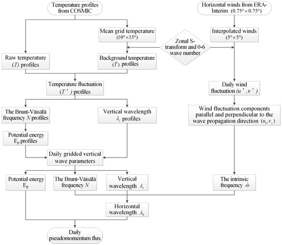
Figure 1.
Flowchart to derive magnitudes of gravity wave (GW) pseudomomentum flux (PMF) from the combination of Constellation Observing System for Meteorology, Ionosphere, and Climate (COSMIC) radio occultation (RO) and ERA-Interim data.
To further analyze the temporal and spatial variations of GW activities, monthly and seasonal means of the 3-dimensional GW parameters are obtained by averaging the gridded daily parameters. The global distribution of the seasonal means of a specific GW parameter for a certain height interval is obtained by averaging the gridded seasonal means vertically, while the temporal variation of zonal monthly means of the magnitudes of GW PMF for a certain height interval is obtained by averaging the zonal monthly means vertically.
3. Results and Analysis
3.1. Validation of the Strategy
The time period of June, July, and August (JJA) 2006 was chosen for validation of the feasibility of the new strategy because the distribution of GW PMFs during this period in some previous studies using RO data independently [6,28] can be used as references in this work. The vertical and horizontal wave parameters for GW activities averaged at the three altitude intervals (20–25 km, 25–30 km, and 30–35 km) are presented to compare the horizontal distribution of GW activities at different altitudes.
As described in Section 2.2, vertical wave parameters are deduced from COSMIC RO temperature profiles. The time-latitude and latitude-altitude distribution patterns of the Brunt–Väisälä frequencies (not shown here) are similar to those of Noersomadi et al. [18], although their altitude interval was 20–27 km. The distributions of Ep and vertical wavelengths, which are prerequisites for determining GW PMF, are presented in Figure 2.
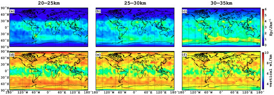
Figure 2.
Global distributions of (a–c) GW potential energy (Ep) and (d–f) vertical wavelengths (vertical wl) during June, July, and August (JJA) 2006 averaged at three altitude intervals: (a,d) 20–25 km, (b,e) 25–30 km, (c,f) and 30–35 km, derived from COSMIC RO temperature data.
Figure 2a–c presents the global distributions of GW Ep during JJA 2006 at the three altitude intervals. The distribution patterns are consistent with previous studies [5,22]. The higher the altitude interval, the larger the Ep values [24,47]. In the lower altitude intervals of 20–25 km and 25–30 km, the maximum values of Ep are found over the northern tropics [12,23], which can be attributed to deep convection over this region [16]. In the 30–35 km altitude interval, the dominant maximums of Ep in the northern tropics are less distinct; instead, a relatively uniform distribution over the tropics appears. In addition, the distributions of Ep at the three altitude intervals all indicate a general enhancement of Ep over the extratropical regions of the Southern Hemisphere (SH), which may be due to the orography and zonal winds over these regions [24]. Specifically, Ep is enhanced over the South of South America, which should be related to the GW activities over the Southern Andes Mountains. This increase extends eastward at all altitudes, more strongly and more persistent at the higher altitudes.
Figure 2d–f show the global distribution of vertical wavelengths of GWs at the three altitude intervals during JJA 2006. Generally, with increased altitude, vertical wavelengths decrease slightly in the mid and high latitudes, while they increase a little in the tropics, which indicates a tendency of more stable global distribution at higher altitudes [32,47]. At all three altitude intervals, the global distributions of averaged vertical wavelengths exhibit minima of around 6 km in the tropics and maximums of around 8 km in the extra-tropics, showing an insignificant difference between the SH and the Northern Hemisphere (NH).
Following the procedures presented in Section 2.3, the ratios of intrinsic frequency to Coriolis frequency are deduced from the gridded horizontal winds of the ERA-Interim reanalysis, and the gridded intrinsic frequencies are obtained accordingly, which are further combined with the Brunt–Väisälä frequencies and the vertical wavelengths deduced from RO temperature data to derive the horizontal wavelengths of GWs. The global distributions of the ratios of intrinsic frequency to Coriolis frequency and the horizontal wavelengths at the three altitude intervals during JJA 2006 are presented in Figure 3. It should be noted that as explained in Section 2.3, the narrow region of ±2° around the equator are excluded in Figure 3 to avoid the singularity at the equator. According, this narrow region is also excluded in all the following figures which present the distributions of the derived GW PMF.
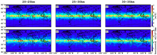
Figure 3.
(a–c) Global distributions of ratio of intrinsic frequency to Coriolis frequency (w/f) deduced from horizontal winds of ERA-Interim reanalysis and (d–f) horizontal wavelengths (horizontal wl) derived accordingly during JJA 2006 averaged at three altitude intervals: (a,d) 20–25 km, (b,e) 25–30 km, and (c,f) 30–35 km.
Figure 3a–c show the global distributions of the ratio of intrinsic frequency to Coriolis frequency averaged at the three altitude intervals during JJA 2006. The distribution patterns of the ratio values are similar to those of Wang et al. [27], with distinct maximums in the low latitudes and much lower values over the other latitudes. The ratio values vary between ~1.2 and ~6.0, showing negligible differences in magnitude at the three altitude intervals. Although the maximum ratio value here (~7.0) is larger than that shown in Wang et al. [27], it is still acceptable because low-intrinsic frequency waves with a ratio smaller than 10 are classified as gravity waves [7,27,45].
Figure 3d–f show the global distributions of horizontal wavelengths averaged at the three altitude intervals during JJA 2006. The horizontal wavelengths vary mainly between ~1000 km and ~3000 km and obtain peak values in the tropics. Furthermore, the horizontal wavelengths decrease from the tropics toward the poles and exhibit a zonal symmetry at all three altitude intervals. The distribution patterns of horizontal wavelengths presented here are consistent with those in previous studies [2,6,27,28] to a large extent, and the negligible discrepancies can be attributed to the different data and methods used.
Based on the horizontal and vertical wave parameters deduced above, the magnitudes of PMF are derived. The global distributions of GW PMF magnitudes and the corresponding zonal means averaged at the three altitude intervals during JJA 2006 are presented in Figure 4.
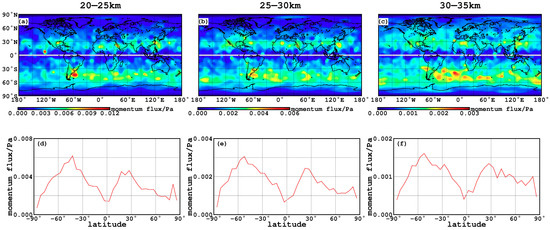
Figure 4.
(a–c) Global distributions and (d–f) zonal means of magnitudes of GW PMF during JJA 2006 averaged at three altitude intervals: (a,d) 20–25 km, (b,e) 25–30 km, and (c,f) 30–35 km, derived from combined COSMIC RO temperature data and horizontal winds of ERA-Interim reanalysis.
A comparison of Figure 4a–c and Figure 4d–f reveals that the magnitudes of PMF generally decrease with increased height, which is consistent with Schmidt et al. [6] and may be due to the upward propagation of gravity wave accompanied by energy and momentum dissipation. Figure 4a–c show that for different altitude intervals, the magnitudes of GW PMF vary significantly, while the horizontal distribution patterns are similar. All altitude-averaged magnitudes of PMF exhibit maximums at a latitude of 40° S–60° S, which is at the edge of the SH polar vortex. The secondary maximums of PMF magnitudes exist at the NH subtropics, and this can be attributed to deep convection [47].
The distribution patterns of PMF presented in Figure 4a–c are generally consistent with those shown in previous studies [2,28,47], while differences exist in the variation range of PMF values and magnitudes of PMF in the low latitudes, which will be discussed further in Section 4.
As to the zonal means of GW PMF, Figure 4d–f show that two peak values exist for all three altitude intervals. One peak value is obtained at around 40° S–60° S, which is about 0.006 Pa, 0.003 Pa, and 0.0016 Pa for the three altitude intervals, respectively, and the other is obtained at the NH subtropics, which is 0.0045 Pa, 0.0025 Pa, and 0.0013 Pa for the three altitude intervals, respectively. The variation patterns of zonal mean GW PMF shown here are consistent with those presented by Ern et al. [32,47] based on temperature observations from Sounding of the Atmosphere using Broadband Emission Radiometry (SABER) and HIRDLS, while the slight enhancements of zonal means of PMF at the tropics that were shown by Schmidt et al. [6] based on COSMIC RO temperature profiles do not exist in our results. The inconsistency between their result and ours can be attributed to the differences in the data sources and methods used to derive GW PMF.
3.2. Seasonal Variations of Magnitude of GW PMF from June 2006 to May 2013
The global distributions of the seasonal means of GW PMF magnitudes from June 2006 to May 2013 at the three altitude intervals are presented in Figure 5. It can be seen that the three altitude intervals share a similar seasonal distribution pattern with enhanced PMF magnitudes in the winter polar vortex. The longitudinal structure of GW PMFs in the summer subtropics is also similar at all three altitude intervals, which can be attributed to the characteristics in the distribution of convective gravity wave sources [47].
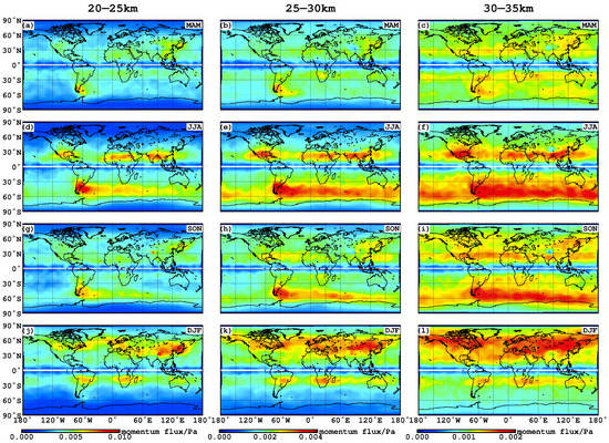
Figure 5.
Global distributions of seasonal mean pseudomomentum fluxes during June 2006 to May 2013: (a–c) March, April, and May (MAM), (d–f) JJA, (g–i) September, October, and November (SON), and (j–l) December, January, and February (DJF), averaged in altitude intervals of (a,d,g,j) 20–25 km, (b,e,h,k) 25–30 km, and (c,f,i,l) 30–35 km, derived from the combined COSMIC RO temperature data and horizontal winds of ERA-Interim reanalysis.
Figure 5 shows that for all three altitude intervals, enhanced values of GW PMF exist from March to October at the Southern Andes and Antarctic Peninsula, which is known to be a prominent source of mountain waves [27]. Another hot spot of GW activity, the Amazon in South America, where strong convective activity occurs, is also discernible in the figure. It should be mentioned that among the three altitude intervals, these GW hot spots are the most discernable at 20–25 km. This is because strong vertical gradient of zonal background winds in height results in enhanced wave-breaking [32,47], which leads to the overall dissipation of gravity waves with altitude, so the variation range of PMF magnitudes is the largest at the lowest altitude interval. The seasonal variations of mean GW PMFs presented here are consistent with the results from SABER and HIRDLS at about 30 km [47]. Besides, the distributions of GW PMF in the subtropical regions are generally symmetric about the equator in March, April, and May (MAM) and September, October, and November (SON), except for strengthened values over topographic hot spots. Specifically, the more enhanced GW PMFs in SON than in MAM over the Southern Andes can be attributed to the inherited influence of strengthened wave activity over this region during JJA [24].
3.3. Time-Latitudinal Distributions of GW PMF Magnitudes from June 2006 to May 2013
Figure 6 shows the time-latitudinal distribution of GW PMF magnitudes at the three altitude intervals during the period from June 2006 to May 2013. Also shown in this figure is the distribution of zonal winds. The interannual variability of PMF values at each altitude interval shown here is a clear seasonal cycle over middle and high latitudes, with peaks of PMF values observed in winter and minima noticed in summer, which is similar to the Ep shown in [24,47]. It can also be seen from Figure 6 that at all three altitude ranges, eastward wind dominates the mid and high latitudes of the winter hemispheres, where the peaks of wind fields coincide with the peaks of GW PMF values, while in the summer hemispheres, the slower westward wind is generally accompanied by lower GW PMF values. The enhanced magnitudes of PMF over latitudes of 40°–60° in the winter hemisphere each year might be partly attributed to waves originating from several mountains in the NH, such as the Rocky Mountains, the Alps, and the Tibetan plateau, the Andes Mountain in the SH, and the winter polar vortex.
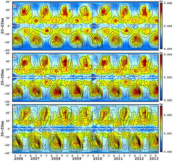
Figure 6.
Time-latitude distributions of GW PMF magnitudes and zonal winds from June 2006 to May 2013 averaged in the altitude intervals (a) 20–25 km, (b) 25–30 km, and (c) 30–35 km. Zonal eastward wind, 0 m/s wind, and westward wind are represented by solid black, solid red, and dashed black lines, respectively. The Capital letters (J O J A) on the horizontal axis represent (July, October, January, and April) during each year.
At each altitude interval, the second maximums of PMF magnitudes exist over the subtropics of the summer hemisphere each year, which can be attributed to deep convection [47]. This enhancement of PMF values is less distinct at higher altitudes due to the decreased PMF magnitude with increased altitude.
Figure 6a shows that at low latitudes between 30° S and 30° N where westward wind dominates, quasi-biennial oscillation (QBO) is evident in the temporal variation of both wind fields and GW PMF values at the altitude range of 20–25 km. Due to the influence of QBO, reversal of the wind field occurs in the tropics and subtropics biennially. It should be mentioned that during the period when no wind reversal occurs, enhanced GW PMF values exist at the peaks of westward wind fields in the subtropics, whereas when wind field reversal occurs, no peak value of GW PMF is obtained, which might be because reversed winds at these latitudes are not strong enough to affect GW activity. Figure 6b,c show that the influence of QBO on wind fields and GW PMF values at the two higher altitude intervals is not as significant as that at the lowest altitude interval.
4. Discussion
To derive GW PMF from RO data independently, triples of RO temperature profiles co-located in both time and space are needed, which makes the strategy feasible only during the early mission time of COSMIC. This is why all the available studies on RO-derived GW PMF focus on the time period of 2006 to 2007. The results presented in this work demonstrate that combining temperature profiles from COSMIC RO and horizontal winds from ERA-Interim reanalysis is a feasible way to study the long-term variations of global GW PMF distribution. The characteristics of GW activities derived using the new strategy are generally consistent with previous works based on RO temperature data, other satellite data, and mode data, although differences in details still exist.
The spatial distributions of GW vertical parameters at the three altitude intervals during JJA 2006 resemble what were shown in previous works [27,28]. The vertical wavelengths of GWs mainly range from 6 km to 8 km, with higher values at mid and high latitudes and lower values at low latitudes. With increased altitude, the vertical wavelengths decrease slightly over mid-high latitudes and increase subtly over the tropics, which is consistent with the variation of GW vertical wavelengths at the altitude range of 25–35 km presented by Ern et al. [32,47]. Besides, the GW vertical wavelengths in extratropical regions of the SH, specifically the winter polar vortex region with enhanced wind speeds [48], are a little larger than those in the extra tropics of the NH [6]. Furthermore, as presented in previous studies [24,28,49], the GW Ep during JJA 2006 generally increased with increased height and the maximum Ep values existed over the northern tropics, and an eastward maximum dragging of GW Ep originating from the Southern Andes Mountains is discernible at all three altitude intervals. The distributions of horizontal wavelength of GWs during JJA 2006 derived from the horizontal wind field of ERA-Interim reanalysis are also similar to what was presented in previous studies [6,12,27].
It should be mentioned that we follow Wang and Alexander [27] and Schmidt et al. [6] to derive the vertical wavelengths of GWs from RO temperature profiles. Although it is pointed out that the elevation angle of the sounding paths and GW aspect ratios in the RO measurement could introduce distortions in the wavelengths [50], these distortion effects are not important to the main results of the vertical wavelength analysis in the present study. The reasons are as follows: Firstly, the biases in the derived vertical wavelength introduced by these distortions could occur for single wave events, while these effects should be small for averaged data [47]. Secondly, as discussed in detail by Yan et al. [51], most of the waves detected in previous GW studies deduced from GPS RO data are inertia-gravity waves, and for COSMIC RO measurement of GWs in the stratosphere, vertical wavelengths are far smaller than horizontal wavelengths. Correspondingly, GW aspect ratios should be very small in most cases.
The magnitudes of GW PMF derived during JJA 2006 are consistent with Ern et al. [32,47]. As to the global distribution of GW PMFs, two latitudinal bands of maximums are remarkable, one at the edge of the SH polar vortex and the other at the NH subtropics, which is consistent with Ern et al. [2,32,47]. It should be pointed out that the variation ranges of PMF magnitudes during JJA 2006 derived in the present study (0–0.012 Pa for 20–25 km, 0–0.006 Pa for 25–30 km, and 0–0.003 Pa for 30–35 km) are different from those shown in Wang et al. [27] and Faber et al. [28]. This is acceptable considering that although they both derived GW PMF based independently on RO temperature data, significant differences in PMF magnitudes exist between these two studies. In Wang et al. [27], the PMF magnitudes during DJF 2006–2007 for the altitude range of 17.5–22.5 km vary between 0.055 mPa and 0.33 mPa, while in Faber et al. [28], the PMF values for the altitude range of 20–30 km during both JJA 2006 and DJF 2006–2007 vary between 0 mPa and 3 mPa. The discrepancies between our results and theirs can be attribute to the differences in data sources, altitude ranges studied, and methods applied to derive PMF. Another notable issue is that the PMF values derived in the present study are smaller in the low latitudes compared with the mid and high latitudes, which is consistent with the PMF distribution pattern derived using United Kingdom Met Office (UKMO) winds [2], but different from those derived using satellite limb soundings from HIRDLS and those from SABER [32,47] and those derived using the RO temperature data independently [6,27,28]. The inclusion of model wind data in the derivation of PMF is likely the factor leading to the discrepancies, and further investigations on this will be carried out in the future.
The seasonal variations and time-latitude distributions of GW PMF at the three altitude intervals during the seven years from June 2006 to May 2013 are finally presented based on this new strategy. From the seasonal variations of the global distribution of GW PMF, several hot spots of GW activity are confirmed, including the Amazon in South America, where strong convection occurs; the northwestern Atlantic; and the coasts along the northeastern US and eastern Canada [27]. Both the seasonal and interannual variations reveal that GW PMF is generally enhanced at around 40°–60° in winter hemispheres and in the subtropics of summer hemispheres. What needs to be mentioned is that the strong GW signals over both land and ocean areas of the middle latitudes in winter hemispheres could be partly excited by the baroclinic jet/front waves. Zhang et al. [52] studied the generation of mesoscale gravity waves in upper-tropospheric jet-front systems through model simulations, and found that balance adjustment is likely responsible for generating the mesoscale gravity waves during the life cycle of idealized baroclinic jet–front systems. Mirzaei et al. [53] assessed the impact of moisture on inertia gravity wave generation for an idealized unstable baroclinic wave, and proposed an empirical parameterization scheme for the inertia gravity wave energy. Wei and Zhang [54] and Wei et al. [55] further analyzed the GW spectral characteristics and studied the characteristics and source mechanisms of mesoscale gravity waves in moist baroclinic jet–front systems, and pointed out that the partial enhancements of some particular wave modes may be due to the enhanced wave generation associated with enhanced localized baroclinic instability.
It should be noted that this is the first time dry temperature profiles provided by the COSMIC RO mission, which has global coverage, long-term stability, and high precision, have contributed to the analysis of interannual variations of GW PMF. Although Ern et al. [47] presented interannual variations of GW PMF during 2002–2015 based on temperature data from SABER, only the latitude range 50° S–50° N is observed continuously by SABER, and the altitude of GW PMF derived from SABER data is not below 30 km. Ern et al. [47] also presented interannual variations of GW PMF derived from HIRDLS temperature data, although HIRDLS only observes the latitude range 63° S–80° N and the time period for interannual variation analysis is only three years, from March 2005 to February 2008, due to the availability of data. In comparison, this study presents interannual variations of GW PMF in three altitude ranges between 20 km and 35 km over the whole globe during the period 2006 to 2013. It is revealed that the interannual variation patterns of GW PMF at the three altitude ranges (20–25 km, 25–30 km, and 30–35 km) are similar to that at 30 km altitude presented by Ern et al. [47], while the magnitudes of GW PMF at different altitude ranges vary greatly. The interannual variations of the distribution of GW PMF at the three altitude intervals indicate that PMF maximums usually occur at latitudes around 60° in the winter hemispheres, where eastward winds prevail, and the second maximums of GW PMF exist over the subtropics of the summer hemispheres, where deep convection occurs. Besides, the influence of QBO on both GW PMF and zonal winds is discernible over subtropical regions.
5. Conclusions
A new strategy is presented in the present study to derive GW PMF by combing RO temperature data and model wind data from ERA-Interim. Following this strategy, the vertical wave parameters of GWs are obtained based on RO temperature profiles in the same way as in previous studies, while GW intrinsic frequencies are obtained based on wind data from the reanalysis. So, both data sources contribute to the derivation of horizontal wavelengths and PMF magnitudes. After the feasibility of the strategy is validated by comparing the spatial and temporal distributions of GW parameters derived this way with those presented in previous studies, the characteristics of seasonal and interannual variations of PMF magnitudes at three altitude intervals (20–25 km, 25–30 km, and 30–35 km) over the globe during the seven years from June 2006 to May 2013 are presented and discussed.
It is found that, except the participation of model wind data in the derivation of GW PMF leading to small GW PMF values in the low latitudes, the spatial distribution patterns of GW PMF are generally consistent with those shown in previous studies based on RO temperature data or other satellite data. The comparison of GW PMF at different altitude intervals reveals that PMF magnitude generally decreases with increased height. The seasonal distribution patterns of GW PMF at the three altitude intervals are similar, while the contribution of topography to the strengthened PMF over some specific regions is the most discernible at the lowest altitude interval of 20–25 km. In terms of the altitude range, latitude coverage, and time period, the present work complements the GW PMF interannual variation patterns derived based on satellite observations from SABER and HIRDLS. Interannual variations of the distribution of GW PMF demonstrate that over the mid and high latitudes of the winter hemispheres, the peaks of eastward wind generally coincide with the peaks of GW PMF values, while over the subtropical regions, where deep convection occurs, the second maximums of GW PMF are obtained and the influence of QBO on both GW PMF and zonal winds is discernible.
In our future work, GW activities over hot spots such as the Alps, the southern Andes, and the Amazon in South America during a relatively long period will be considered based on PMF values derived by combing RO data and model data, which will be beneficial for understanding the temporal variations and background mechanism of GW activities in these regions. We also plan to calculate the GW PMFs only based on the ERA-Interim, and then compare those results with the present study in a fair way.
Author Contributions
X.X. and J.L. (Jia Luo) conceptualized the initial idea and experimental design; J.L. (Juan Li) analyzed the data; X.X., J.L. (Juan Li), and J.L. (Jia Luo) wrote the main manuscript text; J.L. (Jia Luo) and D.Y. reviewed and edited the paper.
Funding
This research was funded by the National Natural Science Foundation of China (grant nos. 41774033 and 41774032), the National Key Research and Development Program of China (grant no. 2018YFC1503502), and the National Basic Research Program of China (973 Program) (grant no. 2013CB733302).
Acknowledgments
We thank two anonymous reviewers for their constructive comments and suggestions on the present work. We would like to express our gratitude to the COSMIC Data Analysis and Archive Center (CDAAC) of the University Corporation for Atmospheric Research (UCAR) for providing COSMIC RO data, and the European Centre for Medium-Range Weather Forecasts (ECMWF) for providing ERA-Interim data.
Conflicts of Interest
The authors declare no conflict of interest.
Appendix A
As has been frequently used to derive gravity wave parameters with radiosonde observations [7,8,44], the Stokes method was proposed by Vincent and Frrits [3] and optimized by Eckermannn and Vincent [10] by using Fourier transform of profiles of zonal and meridional wind perturbations over the complete altitude range:
where m is the vertical wave number, and U and V are the peak amplitudes of zonal and meridional wind perturbations, which are expressed in complexes and , with subscript R and I representing the real and imaginary components. Resembling electromagnetic waves, Stokes parameters in the spectral domain are given by:
where A is a constant that can be reduced later, and I, D, P, and Q are parameters related to wave energy and polarization (detailed by Pramitha et al. [8]). From Stokes parameters, we can calculate the direction of wave propagation by:
With it, horizontal wind perturbation components parallel and perpendicular to the wave propagation direction can be obtained by:
Therefore, pre-parameters are ready for the determination of the intrinsic frequency and horizontal wavelength.
References
- Fritts, D.C.; Alexander, M.J. Gravity wave dynamics and effects in the middle atmosphere. Rev. Geophys. 2003, 41. [Google Scholar] [CrossRef]
- Ern, M.; Preusse, P.; Alexander, M.J.; Warner, C.D. Absolute values of gravity wave momentum flux derived from satellite data. J. Geophys. Res. 2004, 109. [Google Scholar] [CrossRef]
- Vincent, R.A.; Fritts, D.C. A Climatology of Gravity-Wave Motions in the Mesopause Region at Adelaide, Australia. J. Atmos. Sci. 1987, 44, 748–760. [Google Scholar] [CrossRef]
- Alexander, M.J.; Geller, M.; McLandress, C.; Polavarapu, S.; Preusse, P.; Sassi, F.; Sato, K.; Eckermann, S.; Ern, M.; Hertzog, A.; et al. Recent developments in gravity-wave effects in climate models and the global distribution of gravity-wave momentum flux from observations and models. Q. J. R. Meteorol. Soc. 2010, 136, 1103–1124. [Google Scholar] [CrossRef]
- Geller, M.A.; Alexander, M.J.; Love, P.T.; Bacmeister, J.; Ern, M.; Hertzog, A.; Manzini, E.; Preusse, P.; Sato, K.; Scaife, A.A.; et al. A Comparison between Gravity Wave Momentum Fluxes in Observations and Climate Models. Am. J. Clim. Chang. 2013, 26, 6383–6405. [Google Scholar] [CrossRef]
- Schmidt, T.; Alexander, S.P.; de la Torre, A. Stratospheric gravity wave momentum flux from radio occultations. J. Geophys. Res. Atmos. 2016, 121, 4443–4467. [Google Scholar] [CrossRef]
- Murphy, D.J.; Alexander, S.P.; Klekociuk, A.R.; Love, P.T.; Vincent, R.A. Radiosonde observations of gravity waves in the lower stratosphere over Davis, Antarctica. J. Geophys. Res. Atmos. 2014, 119, 11973–11996. [Google Scholar] [CrossRef]
- Pramitha, M.; Ratnam, M.V.; Leena, P.P.; Krishna Murthy, B.V.; Vijaya Bhaskar Rao, S. Identification of inertia gravity wave sources observed in the troposphere and the lower stratosphere over a tropical station Gadanki. Atmos. Res. 2016, 176, 202–211. [Google Scholar] [CrossRef]
- Tsuda, T.; Inoue, T.; Kato, S.; Fukao, S.; Fritts, D.C.; Vanzandt, T.E. MST Radar Observations of a Saturated Gravity Wave Spectrum. J. Atmos. Sci. 1989, 46, 2440–2447. [Google Scholar] [CrossRef][Green Version]
- Eckermann, S.D.; Vincent, R.A. Falling sphere observations of anisotropic gravity wave motions in the upper stratosphere over Australia. Pure Appl. Geophys. 1989, 130, 509–532. [Google Scholar] [CrossRef]
- Li, T.; Leblanc, T.; McDermid, I.S.; Wu, D.L.; Dou, X.K.; Wang, S. Seasonal and interannual variability of gravity wave activity revealed by long-term lidar observations over Mauna Loa Observatory, Hawaii. J. Geophys. Res. Atmos. 2010, 115. [Google Scholar] [CrossRef]
- Alexander, M.J.; Gille, J.; Cavanaugh, C.; Coffey, M.; Craig, C.; Eden, T.; Francis, G.; Halvorson, C.; Hannigan, J.; Khosravi, R.; et al. Global estimates of gravity wave momentum flux from High Resolution Dynamics Limb Sounder observations. J. Geophys. Res. Biogeosci. 2008, 113. [Google Scholar] [CrossRef]
- Wu, D.L.; Waters, J.W. Observations of gravity waves with the UARS Microwave Limb Sounder. In Gravity Wave Processes, NATO ASI Series; Hamilton, K., Ed.; Springer: Berlin, Germany, 1997; pp. 103–120. [Google Scholar]
- Rocken, C.; Anthes, R.; Exner, M.; Hunt, D.; Sokolovskiy, S.; Ware, R.; Gorbunov, M.; Schreiner, W.; Feng, D.; Herman, B.; et al. Analysis and validation of GPS/MET data in the neutral atmosphere. J. Geophys. Res. Atmos. 1997, 102, 29849–29866. [Google Scholar] [CrossRef]
- Tsuda, T.; Nishida, M.; Rocken, C.; Ware, R.H. A global morphology of gravity wave activity in the stratosphere revealed by the GPS occultation data (GPS/MET). J. Geophys. Res. Atmos. 2000, 105, 7257–7273. [Google Scholar] [CrossRef]
- Ratnam, M.V. Enhancement of gravity wave activity observed during a major Southern Hemisphere stratospheric warming by CHAMP/GPS measurements. Geophys. Res. Lett. 2004, 31. [Google Scholar] [CrossRef]
- Schmidt, T.; de la Torre, A.; Wickert, J. Global gravity wave activity in the tropopause region from CHAMP radio occultation data. Geophys. Res. Lett. 2008, 35, 428–451. [Google Scholar] [CrossRef]
- Noersomadi; Tsuda, T. Global distribution of vertical wavenumber spectra in the lower stratosphere observed using high-vertical-resolution temperature profiles from COSMIC GPS radio occultation. Ann. Geophys. 2016, 34, 203–213. [Google Scholar] [CrossRef]
- Alexander, S.P.; Tsuda, T.; Kawatani, Y.; Takahashi, M. Global distribution of atmospheric waves in the equatorial upper troposphere and lower stratosphere: COSMIC observations of wave mean flow interactions. J. Geophys. Res. 2008, 113. [Google Scholar] [CrossRef]
- Rapp, M.; Dörnbrack, A.; Kaifler, B. An intercomparison of stratospheric gravity wave potential energy densities from METOP GPS radio occultation measurements and ECMWF model data. Atmos. Meas. Tech. 2018, 11, 1031–1048. [Google Scholar] [CrossRef]
- Nath, D.; Chen, W.; Guharay, A. Climatology of stratospheric gravity waves and their interaction with zonal mean wind over the tropics using GPS RO and ground-based measurements in the two phases of QBO. Theor. Appl. Climatol. 2014, 119, 757–769. [Google Scholar] [CrossRef]
- Tsuda, T.; Hocke, K. Vertical Wave Number Spectrum of Temperature Fluctuations in the Stratosphere using GPS Occultation Data. Q. J. R. Meteorol. Soc. 2002, 80, 925–938. [Google Scholar] [CrossRef][Green Version]
- Wang, L.; Alexander, M.J. Gravity wave activity during stratospheric sudden warmings in the 2007–2008 Northern Hemisphere winter. J. Geophys. Res. 2009, 114. [Google Scholar] [CrossRef]
- Xu, X.H.; Yu, D.C.; Luo, J. The Spatial and Temporal Variability of Global Stratospheric Gravity Waves and Their Activity during Sudden Stratospheric Warming Revealed by COSMIC Measurements. Adv. Atmos. Sci. 2018, 35, 1533–1546. [Google Scholar] [CrossRef]
- Khan, A.; Jin, S. Effect of gravity waves on the tropopause temperature, height and water vapor in Tibet from COSMIC GPS Radio Occultation observations. J. Atmos. Sol. Terr. Phys. 2016, 138–139, 23–31. [Google Scholar] [CrossRef]
- Yu, D.; Xu, X.; Luo, J.; Li, J. On the Relationship between Gravity Waves and Tropopause Height and Temperature over the Globe Revealed by COSMIC Radio Occultation Measurements. Atmosphere 2019, 10, 75. [Google Scholar] [CrossRef]
- Wang, L.; Alexander, M.J. Global estimates of gravity wave parameters from GPS radio occultation temperature data. J. Geophys. Res. Atmos. 2010, 115. [Google Scholar] [CrossRef]
- Faber, A.; Llamedo, P.; Schmidt, T.; de la Torre, A.; Wickert, J. On the determination of gravity wave momentum flux from GPS radio occultation data. Atmos. Meas. Tech. 2013, 6, 3169–3180. [Google Scholar] [CrossRef]
- Alexander, M.J. Global and seasonal variations in three-dimensional gravity wave momentum flux from satellite limb-sounding temperatures. Geophys. Res. Lett. 2015, 42, 6860–6867. [Google Scholar] [CrossRef]
- Hierro, R.; Steiner, A.K.; de la Torre, A.; Alexander, P.; Llamedo, P.; Cremades, P. Orographic and convective gravity waves above the Alps and Andes Mountains during GPS radio occultation events-a case study. Atmos. Meas. Tech. 2018, 11, 3523–3539. [Google Scholar] [CrossRef]
- Preusse, P.; Ern, M.; Bechtold, P.; Eckermann, S.D.; Kalisch, S.; Trinh, Q.T.; Riese, M. Characteristics of gravity waves resolved by ECMWF. Atmos. Chem. Phys. 2014, 14, 10483–10508. [Google Scholar] [CrossRef]
- Ern, M.; Preusse, P.; Gille, J.C.; Hepplewhite, C.L.; Mlynczak, M.G.; Russell, J.M., III; Riese, M. Implications for atmospheric dynamics derived from global observations of gravity wave momentum flux in stratosphere and mesosphere. J. Geophys. Res. Atmos. 2011, 116. [Google Scholar] [CrossRef]
- Wei, J.; Bölöni, G.; Achatz, U. Efficient modeling of the interaction of mesoscale gravity waves with unbalanced large-scale flows: Pseudomomentum-flux convergence versus direct approach. J. Atmos. Sci. 2019, 76, 2715–2738. [Google Scholar] [CrossRef]
- Anthes, R.A.; Ector, D.; Hunt, D.C.; Kuo, Y.H.; Liu, H.; Manning, K.; McCormick, C.; Meehan, T.K.; Randel, W.J.; Rocken, C.; et al. The COSMIC/FORMOSAT-3 mission: Early results. Bull. Am. Meteorol. Soc. 2008, 89, 313–333. [Google Scholar] [CrossRef]
- Fong, C.J.; Shiau, W.T.; Lin, C.T.; Kuo, T.C.; Chu, C.H.; Yang, S.K.; Yen, N.L.; Chen, S.S.; Kuo, Y.H.; Liou, Y.A.; et al. Constellation Deployment for the FORMOSAT-3/COSMIC Mission. IEEE. Trans. Geosci. Remote Sens. 2008, 46, 3367–3379. [Google Scholar] [CrossRef]
- Fong, C.J.; Yang, S.K.; Chu, C.H.; Huang, C.Y.; Yeh, J.J.; Lin, C.T.; Kuo, T.C.; Liu, T.Y.; Yen, N.L.; Chen, S.S.; et al. FORMOSAT-3/COSMIC Constellation Spacecraft System Performance: After One Year in Orbit. IEEE. Trans. Geosci. Remote Sens. 2008, 46, 3380–3394. [Google Scholar] [CrossRef]
- Tsuda, T.; Lin, X.; Hayashi, H. Analysis of vertical wave number spectrum of atmospheric gravity waves in the stratosphere using COSMIC GPS radio occultation data. Atmos. Meas. Tech. 2011, 4, 1627–1636. [Google Scholar] [CrossRef]
- Dee, D.P.; Uppala, S.M.; Simmons, A.J.; Berrisford, P.; Poli, P.; Kobayashi, S.; Andrae, U.; Balmaseda, M.A.; Balsamo, G.; Bauer, P.; et al. The ERA-Interim reanalysis: Configuration and performance of the data assimilation system. Q. J. R. Meteorol. Soc. 2011, 137, 553–597. [Google Scholar] [CrossRef]
- Stockwell, R.G.; Mansinha, L.; Lowe, R.P. Localization of the complex spectrum: The S transform. IEEE. Trans. Signal. Process. 1996, 44, 998–1001. [Google Scholar] [CrossRef]
- Zeng, Z.; Randel, W.; Sokolovskiy, S.; Deser, C.; Kuo, Y.H.; Hagan, M.; Du, J.; Ward, W. Detection of migrating diurnal tide in the tropical upper troposphere and lower stratosphere using the Challenging Minisatellite Payload radio occultation data. J. Geophys. Res. Atmos. 2008, 113, D03102. [Google Scholar] [CrossRef]
- Preusse, P.; Dörnbrack, A.; Eckermann, S.D.; Riese, M.; Schaeler, B.; Bacmeister, J.T.; Broutman, D.; Grossmann, K.U. Space-based measurements of stratospheric mountain waves by CRISTA 1. Sensitivity, analysis method, and a case study. J. Geophys. Res. Atmos. 2002, 107, CRI 6–1–CRI 6–23. [Google Scholar] [CrossRef]
- John, S.R.; Kumar, K.K. A discussion on the methods of extracting gravity wave perturbations from space-based measurements. Geophys. Res. Lett. 2013, 40, 2406–2410. [Google Scholar] [CrossRef]
- Guest, F.M.; Reeder, M.J.; Marks, C.J.; Karoly, D.J. Inertia–Gravity Waves Observed in the Lower Stratosphere over Macquarie Island. J. Atmos. Sci. 2000, 57, 737–752. [Google Scholar] [CrossRef]
- Serafimovich, A.; Hoffmann, P.; Peters, D.; Lehmann, V. Investigation of inertia-gravity waves in the upper troposphere/lower stratosphere over Northern Germany observed with collocated VHF/UHF radars. Atmos. Chem. Phys. 2005, 5, 295–310. [Google Scholar] [CrossRef]
- Chen, L.; Bian, J.C.; Liu, Y.; Bai, Z.X.; Qiao, S. Statistical analysis of inertial gravity wave parameters in the lower stratosphere over Northern China. Clim. Dyn. 2018, 52, 563–575. [Google Scholar] [CrossRef]
- Ehard, B.; Kaifler, B.; Kaifler, N.; Rapp, M. Evaluation of methods for gravity wave extraction from middle-atmospheric lidar temperature measurements. Atmos. Meas. Tech. 2015, 8, 4645–4655. [Google Scholar] [CrossRef]
- Ern, M.; Trinh, Q.T.; Preusse, P.; Gille, J.C.; Mlynczak, M.G.; Russell, J.M., III; Riese, M. GRACILE: A comprehensive climatology of atmospheric gravity wave parameters based on satellite limb soundings. Earth. Syst. Sci. Data 2018, 10, 857–892. [Google Scholar] [CrossRef]
- Yan, X.; Arnold, N.; Remedios, J. Global observations of gravity waves from High Resolution Dynamics Limb Sounder temperature measurements: A yearlong record of temperature amplitude and vertical wavelength. J. Geophys. Res. 2010, 115. [Google Scholar] [CrossRef]
- Khaykin, S.M.; Hauchecorne, A.; Mzé, N.; Keckhut, P. Seasonal variation of gravity wave activity at midlatitudes from 7 years of COSMIC GPS and Rayleigh lidar temperature observations. Geophys. Res. Lett. 2015, 42, 1251–1258. [Google Scholar] [CrossRef]
- De la Torre, A.; Alexander, P.; Schmidt, T.; Llamedo, P.; Hierro, R. On the distortions in calculated GW parameters during slanted atmospheric soundings. Atmos. Meas. Tech. 2018, 11, 1363–1375. [Google Scholar] [CrossRef]
- Yan, Y.Y.; Zhang, S.D.; Huang, C.M.; Huang, K.M.; Gong, Y.; Gan, Q. The vertical wave number spectra of potential energy density in the stratosphere deduced from the COSMIC satellite observation. Q. J. R. Meteorol. Soc. 2019, 145, 318–336. [Google Scholar] [CrossRef]
- Zhang, F. Generation of mesoscale gravity waves in upper-tropospheric jet-front systems. J. Atmos. Sci. 2004, 61, 440–457. [Google Scholar] [CrossRef]
- Mirzaei, M.; Zülicke, C.; Mohebalhojeh, A.R.; Ahmadi-Givi, F.; Plougonven, R. Structure, energy, and parameterization of inertia–gravity waves in dry and moist simulations of a baroclinic wave life cycle. J. Atmos. Sci. 2014, 71, 2390–2414. [Google Scholar] [CrossRef]
- Wei, J.; Zhang, F. Mesoscale Gravity Waves in Moist Baroclinic Jet–Front Systems. J. Atmos. Sci. 2014, 71, 929–952. [Google Scholar] [CrossRef]
- Wei, J.; Zhang, F.; Richter, J.H. An Analysis of Gravity Wave Spectral Characteristics in Moist Baroclinic Jet-Front Systems. J. Atmos. Sci. 2016, 73, 3133–3155. [Google Scholar] [CrossRef]
© 2019 by the authors. Licensee MDPI, Basel, Switzerland. This article is an open access article distributed under the terms and conditions of the Creative Commons Attribution (CC BY) license (http://creativecommons.org/licenses/by/4.0/).