Measurements and Modeling of the Full Rain Drop Size Distribution

Abstract

The raindrop size distribution (DSD) is fundamental for quantitative precipitation estimation (QPE) and in numerical modeling of microphysical processes. Conventional disdrometers cannot capture the small drop end, in particular the drizzle mode which controls collisional processes as well as evaporation. To overcome this limitation, the DSD measurements were made using (i) a high-resolution (50 microns) meteorological particle spectrometer to capture the small drop end, and (ii) a 2D video disdrometer for larger drops. Measurements were made in two climatically different regions, namely Greeley, Colorado, and Huntsville, Alabama. To model the DSDs, a formulation based on (a) double-moment normalization and (b) the generalized gamma (GG) model to describe the generic shape with two shape parameters was used. A total of 4550 three-minute DSDs were used to assess the size-resolved fidelity of this model by direct comparison with the measurements demonstrating the suitability of the GG distribution. The shape stability of the normalized DSD was demonstrated across different rain types and intensities. Finally, for a tropical storm case, the co-variabilities of the two main DSD parameters (normalized intercept and mass-weighted mean diameter) were compared with those derived from the dual-frequency precipitation radar onboard the global precipitation mission satellite.

1. Introduction

Accurate measurement and characterization of the raindrop size distribution (DSD) is crucial for many applications in meteorology, ranging from quantitative precipitation estimation (QPE) to numerical modeling of microphysical processes of rain formation and evolution. DSD models have largely been based on surface measurements of rainfall in a wide variety of rain types, intensities, and climatologies mainly based on commercial disdrometers such as Joss-Waldvogel [1], 2D-video (2DVD; [2,3]), Parsivel [4], or the ODM optical disdrometer [5]. It is well-known that these instruments cannot accurately characterize the small drop end of the DSD (D < 0.7 mm or so) due to limited resolution, poor sensitivity, or other instrument-related problems (e.g., [6,7,8]). From the viewpoint of radar QPE, the small drop end has not been of much interest as the radar observables are dominated by the higher order moments of the DSD. On the other hand, microphysical processes such as collisionally forced drop breakup, coalescence, evaporation, and sedimentation, which ultimately shape the DSD (over the entire range of sizes), depend on the lower order moments. Thus, measurement of the “full” DSD is needed, covering the nearly two orders of magnitude of the size range from drizzle sizes to precipitation sizes (100 microns to 7 mm) to characterize different possible shapes of small, medium, and large drop regimes. One way has been to collocate a high-resolution (50 microns) optical array probe (MPS: meteorological particle spectrometer) for the small drop end (100 microns to 1.5 mm) and the moderate resolution (170 microns) 2DVD for sizes >0.7 mm [9,10,11]. Good agreement in the overlapping size range between the two instruments places confidence in the data quality (e.g., calibration, instrument errors, or software processing) over the entire size range, which is necessary for accurate modeling of the DSD. The DSD obtained via merging the data from the two instruments will be referred to as the “composite” spectra.

The scaling normalization of the DSD as proposed in [12] and the generalization given in [13] to include double-moment normalization [14,15] using two reference moments has proven to be useful to arrive at the intrinsic or generic shape of the distribution (referred to as h(x) defined later in Section 2, Equation (2)). The hypothesis is that a large part of the DSD variability (around 80%; [16]) can be accounted for by the two reference moments, with variations in h(x) playing a secondary role to the extent that the shape of h(x) may be considered as “stable” or “invariant” [17]. In other words, after normalization, the scatter in h(x) is greatly reduced, enabling a good fit to its shape relative to more commonly used models such as exponential, standard gamma, and log-normal [15,18,19,20]. The use of three moments in the normalization will even further reduce the scatter in h(x) [16,21]. In this study, we use the generalized gamma (GG) model, whose properties are such that the prior forms are special cases (exponential and standard gamma) or limiting cases (log-normal). Furthermore, there are strong theoretical grounds for the GG based on maximizing the relative entropy [22] subject to moment constraints. One important feature of the GG is that the form is retained under coordinate transformation of the type m = αD^β, where m is the particle mass, which is not true for exponential, standard gamma, or log-normal distributions [23]. Although the GG model for h(x) involves two shape parameters (as opposed to one shape parameter for the standard gamma), the improved flexibility to simultaneously fit (with high fidelity) the shape at the drizzle drop and large drop ends together with the often observed “shoulder” region in between is a distinct advantage [10], with the caveat that the full DSD is measured (otherwise truncation at the small drop end will distort the shape giving erroneous estimates of the shape parameters).

In this paper, we measure the full DSD spectra in variety of rain types and intensities using collocated 2DVD and MPS disdrometers from two campaigns: (i) a six-month campaign in 2015 conducted in Greeley, Colorado, (GXY), and (ii) a longer campaign in Huntsville, Alabama (HSV), which commenced in 2016. The “composite” DSDs are constructed using measurements from both instruments, as reported in [9]. The resulting DSD spectra highlighted the need for a flexible model to represent the intrinsic shape, and subsequently, Thurai and Bringi [10] considered the GG formulation given in [13] as well as in [24]. Here we extend the evaluation of this model against the measured data from a heuristic perspective (as opposed to statistical hypothesis testing), as well as examine the variations of the two shape parameters in different rain types/intensities.

The paper is organized as follows. In Section 2, we summarize the double-moment normalized version of the GG formulation, followed by a description of data from GXY and HSV in Section 3. Assessment of the fitted model is considered in Section 4, and the range of the shape parameters governing the model are examined in Section 5. Finally, a case event is considered in terms of the DSD characteristics from our ground-based composite DSDs, which are compared with those derived from the dual-frequency precipitation radar onboard the global precipitation mission (GPM) satellite [25]. We end with a brief discussion and conclusions in Section 6.

2. The Generalized Gamma Model

The generalized gamma (GG) model has been used for representing particle size distributions (PSD) for a variety of hydrometeors. They range from cloud droplet and fog DSDs [26,27,28] to ice PSDs [23,29]. The model is also referred to as modified gamma distribution. For rain, the use of GG formulation as a basis for representing DSDs has been somewhat more recent. As mentioned earlier, Auf der Maur [24] and Lee et al. [13] were some of the early publications reported in the literature. Other studies making use of the GG formulation for rain DSDs include Kuo et al. [30] as well as references [10,17].

Following [24], the raindrop size distribution (DSD), represented by N(D), can be expressed as

$$N\left(D\right)=M_0\frac{c\lambda }{\mathsf{\Gamma }\left({\mu }_{GG}\right)}{\left(\lambda D\right)}^{c{\mu }_{GG}-1}\exp \left[-{\left(\lambda D\right)}^c\right]$$

(1)

where M₀ is the zeroth moment (total number of drops per m³) and μ_GG and c are two shape parameters. Both M₀ and λ can be expressed in terms of two reference moments, M_i and M_j [13], leading to the double-moment normalized version of Equation (1), given by

$$N\left(D\right)=N_0\prime h_{GG\left(i,j,\mu ,c\right)}\left(x\right)$$

(2)

where

N₀′ = M_i^{(j + 1)/(j − i)} M_j^{(i + 1)/(i − j)},

D_m’ = (M_j/M_i)^{1/(j − i)},

$$h_{GG\left(i,j,\mu ,c\right)}\left(x\right)=c{\mathsf{\Gamma }}_i^{\frac{\left(j+c{\mu }_{GG}\right)}{\left(i-j\right)}}{\mathsf{\Gamma }}_j^{\frac{\left(-i-c{\mu }_{GG}\right)}{\left(i-j\right)} }{x}^{c{\mu }_{GG}-1}\exp \left[-{\left(\frac{{\mathsf{\Gamma }}_i}{{\mathsf{\Gamma }}_j}\right)}^{\frac{c}{\left(i-j\right)}}{x}^c\right],$$

$${\mathsf{\Gamma }}_i=\mathsf{\Gamma }\left({\mu }_{GG}+\frac{i}{c}\right),$$

$${\mathsf{\Gamma }}_j=\mathsf{\Gamma }\left({\mu }_{GG}+\frac{j}{c}\right),$$

and

$$x=\left(\frac{D}{D_m\prime }\right).$$

If we set i = 3 and j = 4 (as in [14]), then D_m’ becomes equal to D_m, the mass-weighted mean diameter. Thus, Equation (2) can be expressed in compact form as N(D) = N₀′ h(x; µ_GG, c) = M₃/D_m⁴ h(x; µ_GG, c). Any moment of the DSD can be expressed as power laws of the two reference moments (M₃, M₄) and the shape parameters (µ_GG, c); in particular, the lower order moments (M₀, M₁, M₂) which are involved in modeling microphysical processes. Raupach et al. [8] discuss the implications of using other moment-pairs (e.g., M₃ and M₆).

Note also that Equation (2) will reduce to the standard gamma (SG) model for c = 1, defined by the three parameters [N_W, D_m, μ_SG)], where μ_SG = μ_GG − 1 and N_W, the normalized intercept parameter, is simply related to N₀′ via N_W = [4⁴/6]N₀′. Furthermore, Equation (2) further reduces to an exponential distribution when μ_GG is set to 1, i.e., μ_SG = 0. The two shape parameters are determined as follows: the measured DSD spectra used as input to the fitting procedure were constructed by utilizing the corresponding MPS-based N(D) measurements for 0.15 < D ≤ 0.75 mm and the 2DVD-based DSD measurements for D > 0.75 mm, where the averaging window is set to 1 or 3 min (which is a compromise between reducing sampling fluctuations and retaining the physical variations, especially in convective rain). The composite N(D) is then scaled by N₀′ and D is normalized by D_m’ so that h_{GG(i = 3,j = 4,μ,c)} is a function of x. For each composite N(D), the optimal values of μ and c are obtained by minimizing the sum of squared differences between log h_GG and the logarithm of the double-moment normalized composite N(D).

3. Observation Campaigns and Data

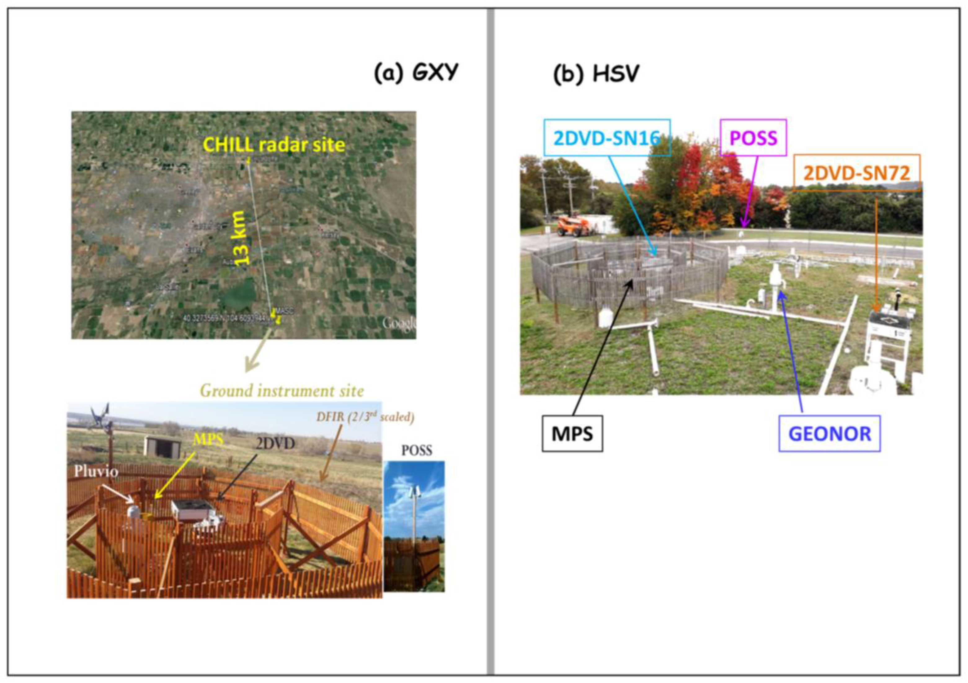
The Greeley campaign was conducted for six months from April to October 2015. The two panels in Figure 1a show the experimental set-up. Both the 2DVD and the MPS were installed inside a 2nd/3rd-scaled double fence inter-comparison reference (DFIR) windshield, as shown in the bottom panel. Also installed inside the DFIR was a second-generation Pluvio weighing-type rain gauge, with a collection area of 200 cm², that utilizes a highly precise load cell to enable measurements of rainfall amounts as low as 0.1 mm with an accuracy of 0.2% [31]. Another instrument installed at the site (outside the double fence) was a precipitation occurrence sensor system (POSS, [32]), which has a much larger sampling volume than those of the 2DVD and the MPS. The ground instrumentation site was 13 km SSE from the CSU-CHILL radar facility [33], as shown in the top panel of Figure 1a.

The Huntsville campaign began in March 2016 and is ongoing. The ground instrumentation set-up was similar to the Greeley campaign, i.e., the 2DVD and the MPS installed inside a 2nd/3rd-scaled DFIR and a POSS outside the fence, as shown in Figure 1b. Additionally, another 2DVD was installed outside the DFIR, primarily to investigate the influence of high winds on drop fall velocities but also to compare with the 2DVD DSD measurements from inside the fence. A Geonor gauge [34] was installed in early 2018. Other collocated instruments include a vertically pointing X-band Doppler radar (XPR) belonging to University of Alabama, Huntsville, as well as a number of meteorological instruments. The ground instrumentation site is located 15 km NE of the ARMOR radar facility operated by UAH [35].

3.1. An Example Event from Greeley

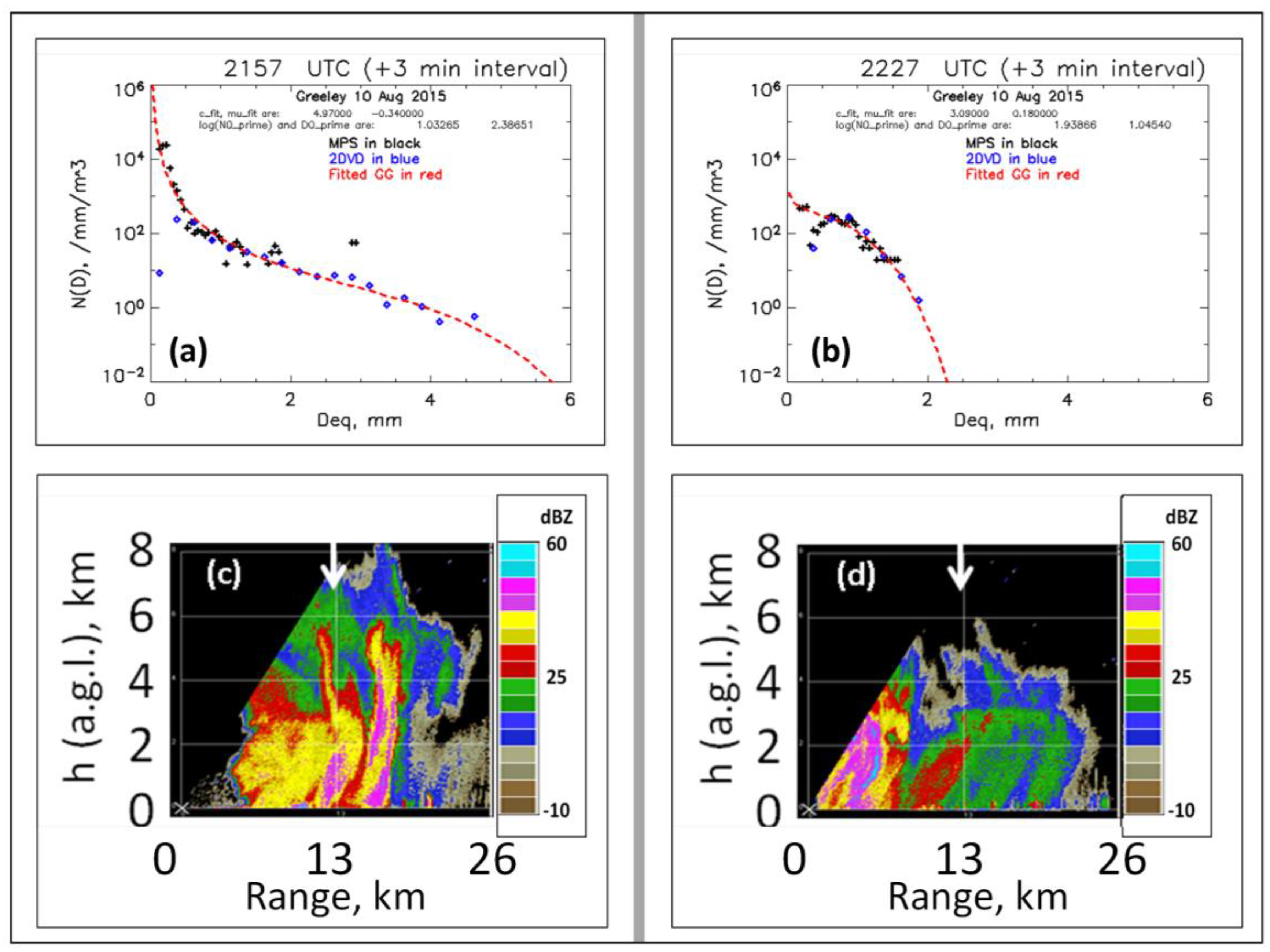
An example event which occurred on 10 August 2015 which lasted for about 1 h over the instrument site during which a convective cell passed over the site is given by Figure 2. Panels (a) and (b) show the measured three-minute DSDs as well as their fitted curves for two time periods, viz. 21:57–22:00 and 22:27–22:30 UTC. The 2DVD-based DSD measurements are shown in blue and the MPS in black. One can see the good overlap between the MPS and the 2DVD measurements in the 0.7 to 1.2 mm size range. Below this range, the underestimate of drop concentration by the 2DVD is also evident. By combining the MPS data for D less than 0.75 mm and the 2DVD data above 0.75 mm, we construct what we term as the “composite” DSD spectra, covering the size range from 150 microns to large raindrops. The red dashed lines show the fitted curves to these composite DSD data based on Equation (2). In both cases, the curves appear to represent the full spectra with high fidelity.

Panels (c) and (d) of Figure 2 show the corresponding S-band CHILL RHI scans made along the azimuth of the instrumentation site. The 13 km range is indicated with white arrows. At 21:57 UTC, the intense convective cell traversed the instrument site, showing reflectivities to 50 dBZ extending to 6 km agl. From Panel (a), we see rather large raindrops (maximum recorded diameter being 4.6 mm), with a D_m value of nearly 2.4 mm. The shape of the DSD for this high Z_e case resembles an equilibrium-like “S”-shaped distribution, for example [36,37], and the double curvature is very well captured by the fitted curve in red. At 22:27 UTC, the deep convection moved north toward the radar and the trailing stratiform rain with embedded weak convection (around 20 dBZ) moving across the instrumented site. Figure 2b shows that N(D) exhibits a non-exponential shape with no evidence of evaporation, which is suggested by the presence of the drizzle mode. The maximum recorded drop diameter is around 2 mm. Here too, the fitted curve captures non-exponential features with high fidelity.

3.2. An Example Event from Huntsville

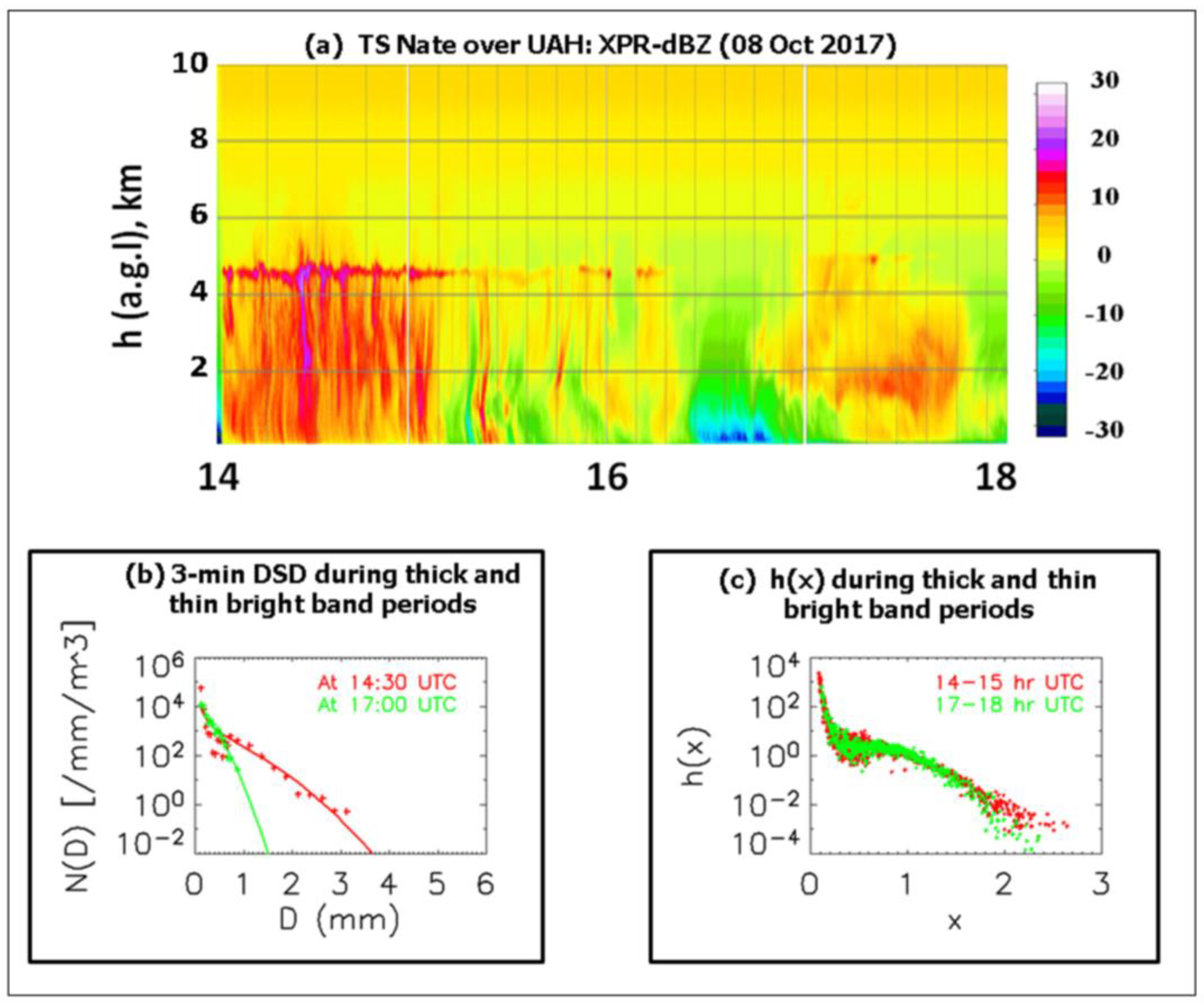
The example shown in Figure 3a covers a four-hour time period during the passage of tropical storm Nate over the instrumented site. Although Nate was a category-1 hurricane during landfall, it had weakened in strength by the time it reached Huntsville. Panel (a) shows the time-height cross sections of reflectivity from the vertical pointing X-band Doppler radar (XPR). The attenuation due to rain leaking inside the radome and on to the antenna was quite excessive during this event yet the bright band is clear between 4 and 5 km agl. Note also the thickness and intensity of the bright band varied during this time period.

In Panel (b), we show the three-minute composite DSD data for two different time periods and their fitted curves. The red curve and the red points correspond to a relatively intense bright-band period at around 14:30 UTC, whilst the green curve and the green points correspond to 17:00 UTC with weak or no bright band and possibly dominated by warm rain processes (K. Knupp, personal communication). Once again, in both cases, we see the fitted curves showing close representation of the measured DSDs. Note also the larger drop sizes for the 14:30 UTC period (thick bright band) which is consistent with Gatlin et al. [38] who showed good correlation between the bright-band thickness and the increasing drop sizes in the rainshaft below. The trends in D_max compared to those we found for D_m suggest that the tail of the DSD is much more affected by changes in the ML characteristics. Consequently, radar rainfall estimators based on reflectivity (i.e., highly sensitive to the tail of the DSD) should be correspondingly more variable with changes in ML thickness and height compared to those estimators that utilize K_DP and Z_DR that are less sensitive to D_max.

Some previous studies, for example [17], have examined the double-moment normalized intrinsic shape represented by the function h(x) for various rain types and found h(x) to be relatively stable in stratiform rain. In an attempt to examine this feature in the rain bands of Nate, three-minute DSDs during the thick (1400–1500 UTC) and warm rain (1700–1800 UTC) periods were used to derive h(x) versus x where x = D/D_m’ and h(x) = N(D)/N₀′ (see Section 2), all derived from the DSD data themselves. The results are plotted in Panel (c) of Figure 3. They exhibit little variation between the thick bright-band and warm rain periods, except for x > 1.8. Also noteworthy is that the shape of h(x) appears to be rather similar to those reported in [13] for stratiform rain (e.g., their Figure 7a) where they also used M₃ and M₄ as reference moments, even though their data were obtained from POSS measurements in Ontario, Canada.

4. Assessment of Fits

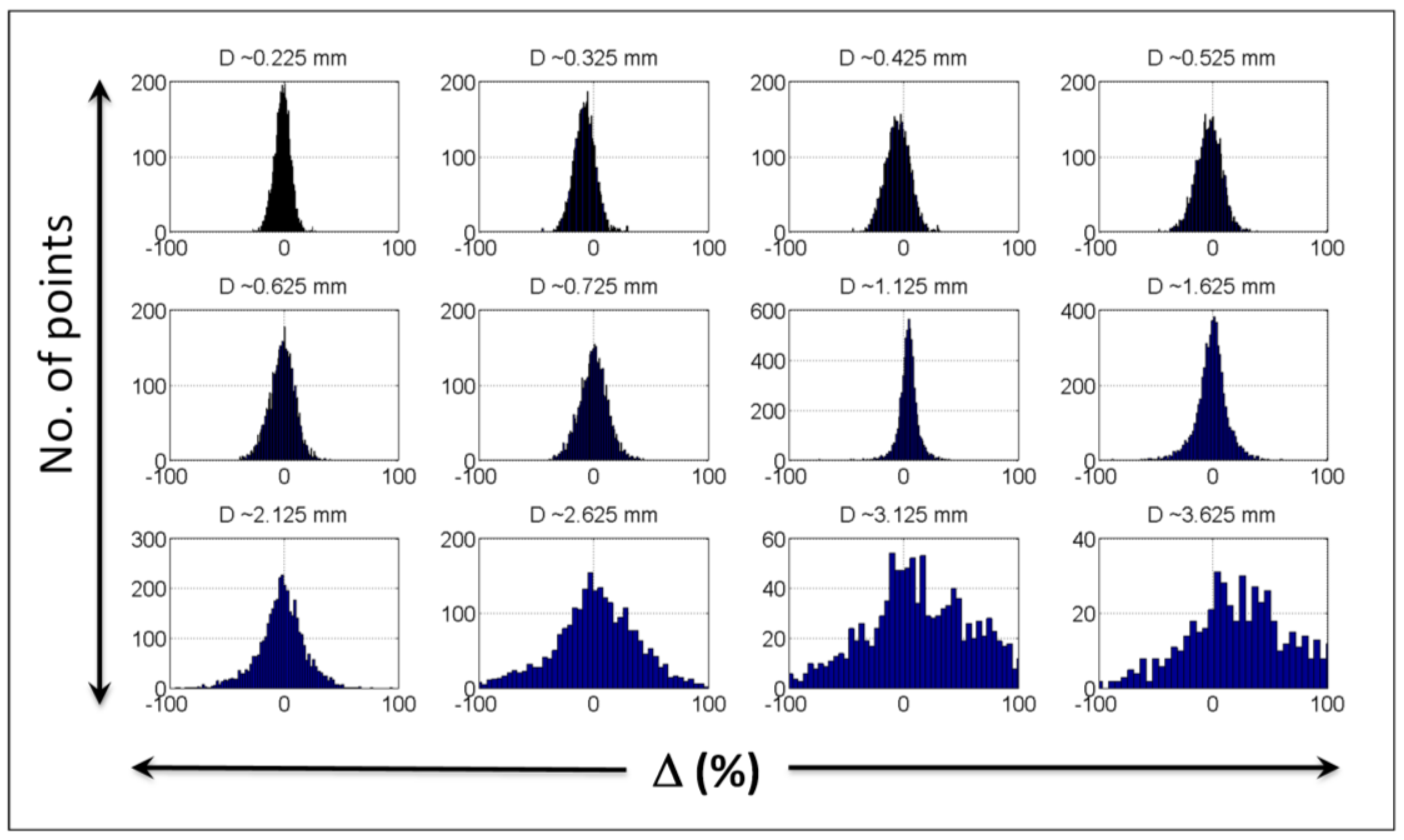
The illustrative examples shown above have highlighted that h(x) based on the composite DSDs can be fitted to the generalized gamma form with the two shape parameters (μ_GG, c) with high fidelity. Further examples can be seen in [10]. To assess the goodness of fit, a heuristic method is adopted based on the difference (Δ) between the measured composite DSD (at 1 min temporal averaging) and the optimized GG fit. The total number of DSDs is 12,177 taken from both GXY and HSV sites. The Δ is calculated for each size bin and the relative deviation (or bias), which is the ratio of Δ to the measured value, is computed. The histogram of this ratio (actually the logarithmic difference) is shown in Figure 4. For each histogram, the center diameter of the bin (in mm) is shown on top. For the small drops, the bin width was set at 0.05 mm (based on MPS resolution), and for the larger drops (>0.75 mm), the bin width was set to 0.25 mm. In most cases, the mean of the relative bias can be noted to be fairly close to 0 (mostly < 15%) and quite symmetric. For D < 2.125 mm, the histograms are Gaussian-like with low spectral width and negligible skewness. For larger diameters, the histograms are “noisy” and do not appear to have “converged” due to decreasing number of sampled drops (i.e., manifestation of sampling errors [39]). For example, the standard deviation for the 0.625 mm drops was 11%, and the number of points was 4263, whereas for 3.625 mm these values were 65% and 594, respectively. Despite the broadening of the histograms for drop sizes >2.125 mm, in general, they illustrate the overall “fidelity” of the fitted GG model to the composite DSDs.

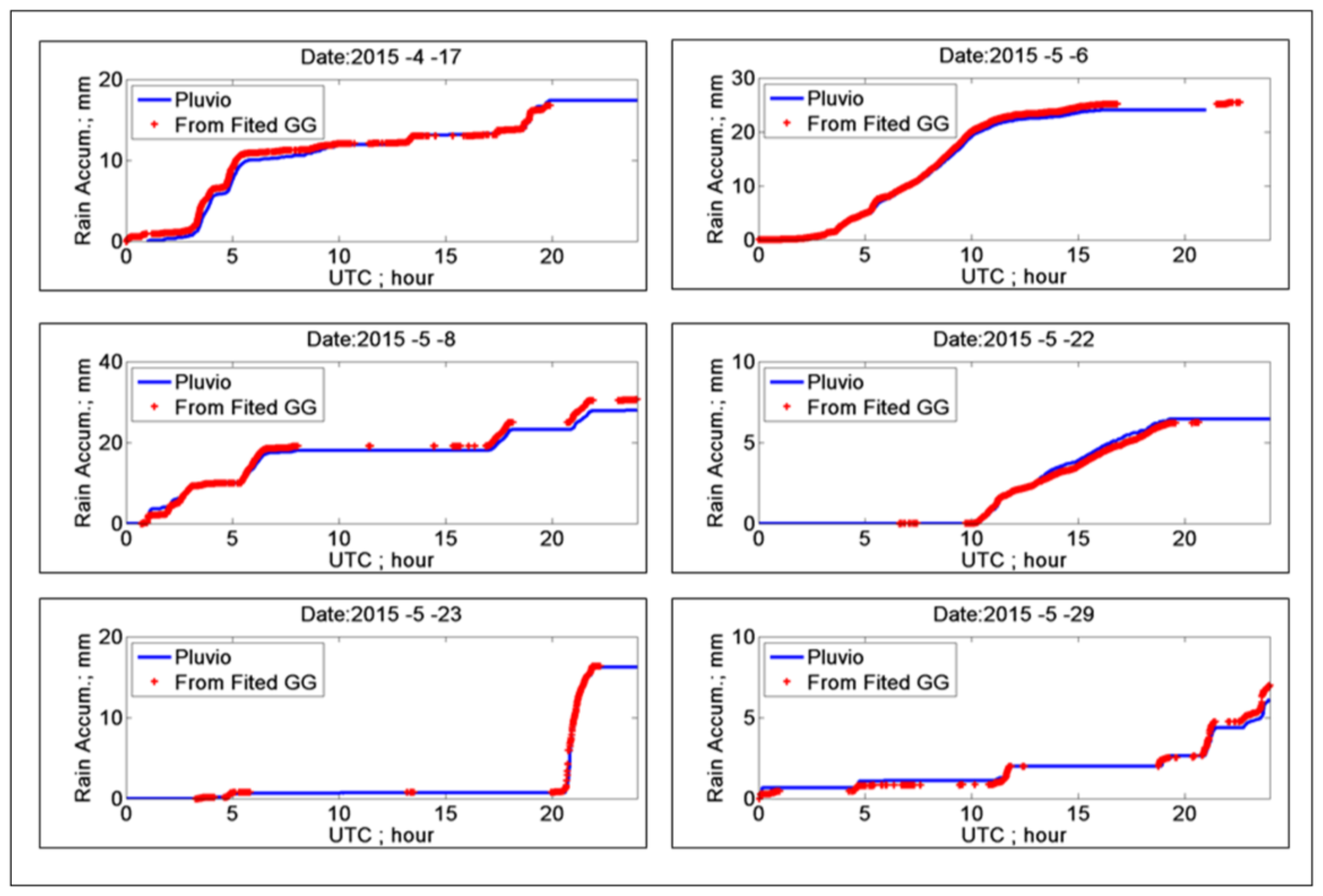
As a further illustration (and as a “sanity” check) of how well the GG-fits represent the DSDs, we consider the first six events recorded during the Greeley campaign. As mentioned earlier, a Pluvio gauge [31] was collocated with the MPS-2DVD instruments. Figure 5 shows time series of rain accumulations from Pluvio measurements for these six events (blue curves). The rain accumulations derived from the GG fits are also plotted (red points). Appropriate corrections needed to be applied to drop fall velocities used in the calculation of the rain rates/accumulations because of the reduced pressure at the 1.4 km height above sea level for the GXY site [40]. In all six cases, the GG-fitted accumulations closely track the Pluvio accumulations with negligible overall bias.

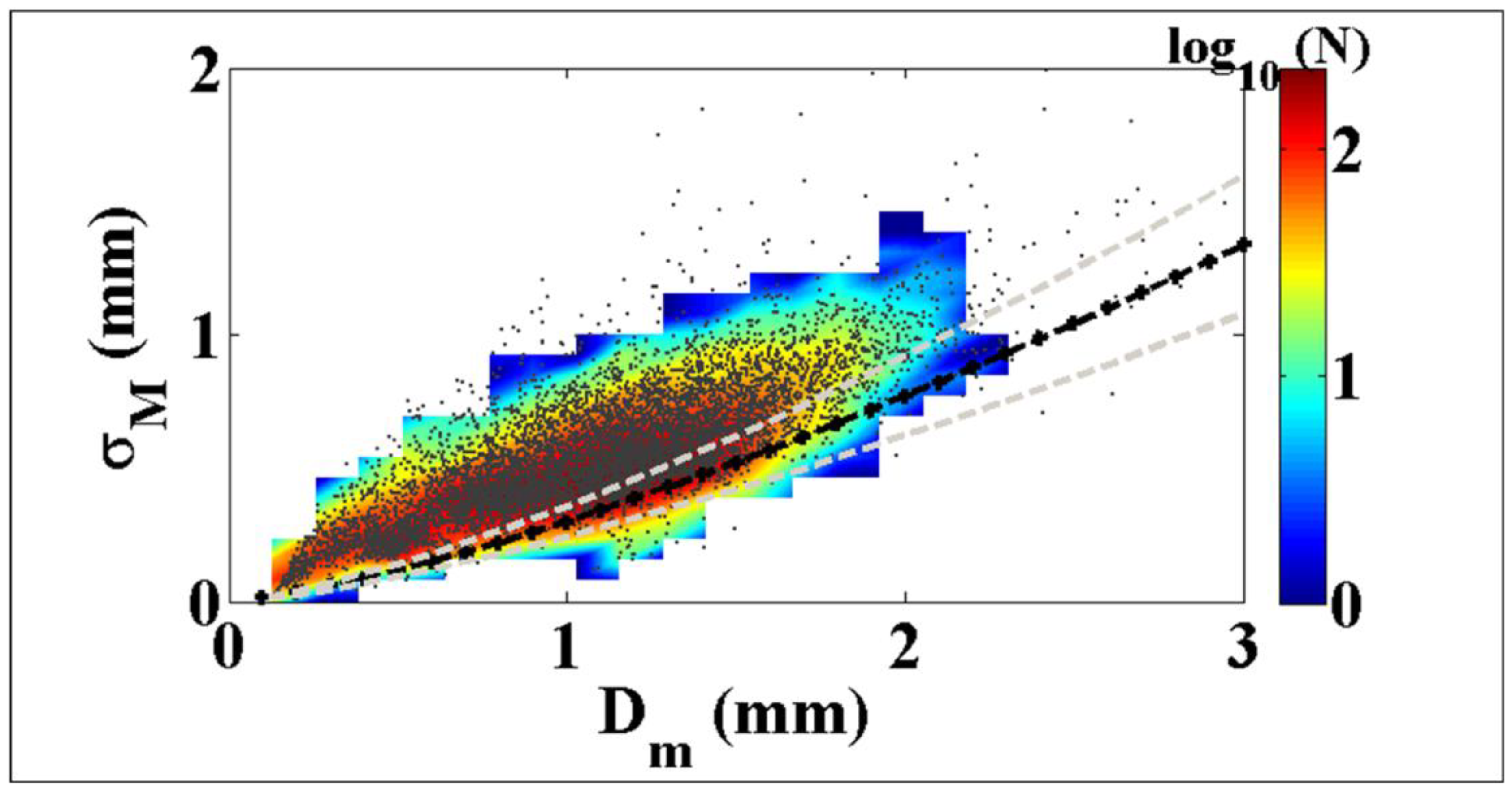
As a further illustration of the representativeness of the GG-fits in terms of higher order moments (M₃ and higher) and moment ratios, in Figure 6 we show the variation of versus (the standard deviation of mass spectrum; [41]) derived for the same 12,177 one-minute DSDs. The color intensity plot represents the contoured 2D-frequency of occurrences based on the measured composite DSDs, whereas those derived from the GG fits are shown as black dots. Most of these latter points lie well within the “higher frequency of occurrence region,” giving further confirmation of the GG fits in terms of higher-order moments. We have also included in Figure 6 three curves, one in black and the other two in gray. They represent Equations (22)–(24), given in [42] which were based on 2DVD data alone (small drops being truncated) with the black curve showing the most likely variation and the gray lines showing the upper and lower bounds. The underestimation of σ_M for a given D_m in black/grey curves is largely due to the inability of the 2DVD to accurately measure the small drop end of the spectrum.

5. μ–c Variations and Shape Stability

So far, we have seen that the GG is a suitable model for representing the measured composite DSD datasets. We have chosen M₃ and M₄ as reference moments in order to be compatible with Testud et al. [14] and to compare with the more widely used standard gamma model [43]. One can also use other moment-pairs depending on the application. For example, M₃ and M₆ have been shown to be more appropriate for polarimetric radar retrievals [13,44]. In any case, as can be gleaned from Equation (2), utilizing these two reference moments along with the fitted h(x) function, it becomes possible to closely model the full DSD spectra together with all its moments.

For a given measured DSD, the fitted h_GG(x) depends on the two shape parameters [μ, c], and it is of fundamental importance to examine the variability of these parameters in various rain types and intensities. Earlier in Figure 3c, we saw that the h(x) derived from the composite measured DSDs was almost stable during the stratiform and warm rain periods of tropical storm Nate. This in turn points to the stability of [μ, c] during these periods with very different microphysics. Figure 7a shows the frequency of occurrence of the fitted [μ, c] as contoured intensity plot derived for all the three-minute DSDs from GXY and HSV combined (4541 in total). The color scale represents the number of points on a log scale. The most probable values in the µ–c plane are (−0.5, 3.9). Over 70% of the fitted μ values are in the range from 0 to −0.6. The c values, on the other hand, show a broader range with a peak close to 4. Note also that the standard gamma value of c = 1 is not close to the region of peak intensity in Figure 7a. Less than 6% of the cases had 0.75 < c < 1.25. This clearly indicates that, for the vast majority of cases, the standard gamma is not an appropriate model to represent the full DSD spectra.

Also examined were the variation of μ and c with D_m. No correlation between μ and D_m was found (not shown here) using the combined DSD data from GXY and HSV. Figure 7b also from the GXY and HSV data shows no correlation between c with D_m. For the HSV dataset alone, the c versus D_m shows an interesting feature (Figure 7c), viz., the most probable range of values in the (c, D_m) plane are, respectively, 2–4 and 1.0–1.8 mm. Note also that D_m rarely goes below 0.5 mm. The implication of these features is not clear. However, the frequency of occurrence of stratiform rain is expected to be typically very high (around 70–80%), which dominates the statistics. One could speculate that the range of c between 2 and 4 may be representative of stratiform rain in the sub-tropical climate of HSV. Note that c controls the shape at the large drop end when µ is around −0.5 (which, in turn, controls the shape at the small drop end). The lower bound for D_m around 0.5 mm could be related to higher sub-cloud relative humidity, which inhibits evaporation of small drops.

The stability of h(x) has been demonstrated using Parsivel disdrometer data for stratiform rain in [17], but the small drop end could not be accurately characterized by the Parsivel leading to a typical convex down shape (or, positive average µ in the range 3–4). In Figure 7d, we show the stability of h_GG(x) at the Greeley site (GXY) with contoured frequency of occurrence plots of h(x) for all one-minute DSDs during rain-only events. Overlaid onto the plot is the “modal” h_GG(x) obtained from the modal values of µ and c from the optimized fits to the individual 1-min-measured DSDs (other methods of arriving at the “modal” h(x) are described in [8]). Note the small drop end (x < 0.5) has a concave up shape, while the large drop end (x > 2) falls faster than an equivalent exponential (e.g., due to drop break-up). The “modal” h(x) goes through the “most probable” regions, at least for x up to 2. For x in the 0.5–1 region, a somewhat more broadened h(x) can be seen perhaps due (partly) to increased variability in h(x) in the overlap region of the two instruments (see, also, [8]).

6. A GPM Overpass Case

Finally, we consider an overpass case of the Global Precipitation Measurement (GPM) satellite [45] over a swath of Northern Alabama. One of the main instruments onboard the satellite is the dual-frequency precipitation radar (DPR), which consists of a Ku-band (13.6 GHz) and a Ka-band (35 GHz) precipitation radar [46]. The radars have the same 4 km footprint for a given location on the earth’s surface.

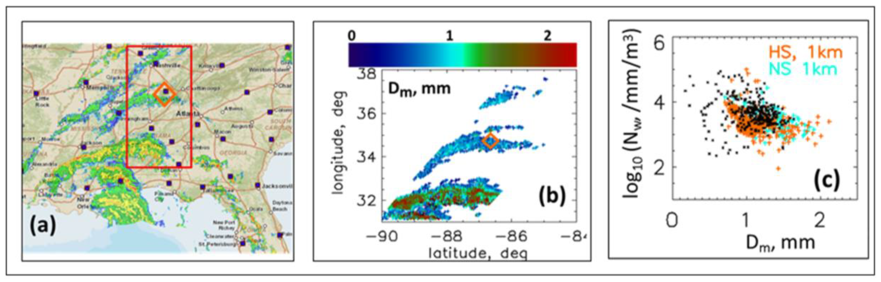
During tropical storm Nate (which had made landfall earlier along the northern gulf coast and had moved quickly northward reducing in strength toward Northern Alabama), the GPM overpass captured the outer bands on 7 October 2017 between 2300 and 2315 UTC. Figure 8a shows the composite WSR-88D radar image of reflectivity at the GPM overpass time, and Figure 8b shows the spatial distribution of the mass-weighted mean diameter (D_m) retrieved from DPR for pixels from the red box in Panel (a). Three “branches” of the outer bands are noted during the overpass time; however, the more intense branch to the south did not traverse the disdrometer site until the next day 8 October 2017 with rain lasting for > 6 h in HSV (similar to Figure 3a). Assuming that the rain bands sampled by the DPR (Figure 8b) over an extended area during the overpass time retained similar microphysics to the bands that traversed the HSV site the next day, the co-variability in the (N_w, D_m) plane can be compared to determine if the trends are similar.

Figure 8c shows the DPR-based retrievals of the DSD parameters, N_w and D_m, derived from the normal scan mode (NS) and high sensitivity mode (HS) at an altitude of 1 km agl [47]. They are restricted to regions above 32° longitude. Overlaid as black points are the values from the 3 min composite DSDs for an 8 h period of the rain bands over the HSV site (part of these data are shown in Figure 3a). Although the composite DSDs exhibit more DSDs with lower D_m, there are similar co-variabilities in the (N_w, D_m) plane compared to those derived from DPR, which is encouraging, especially given the errors in comparing point measurements at the surface (over the entire duration of Nate over HSV) to areal-averaged DPR retrievals (over an extended area but encompassing a short duration of the overpass) at an altitude of 1 km agl. The most probable values of µ ≈ −0.5 and c in the range of 2–4 (not shown here) obtained by fitting the composite DSDs based on > 6 h of rainfall from the outer bands of Nate (based on modal fits to h(x) in Figure 3c) are consistent with Figure 7a,b, which are based on a very large data set encompassing two different climatologies. The implication is that the intrinsic h(x) is stable in shape and that the DSD variability can be largely accounted for by the co-variability in the (N_W, D_m) plane.

7. Discussion and Conclusions

Our measurements, using a high-resolution (50 microns) optical array probe (MPS) collocated with a moderate resolution (170 microns) 2DVD to cover the entire size range from 100 microns upward, have highlighted the suitability of the generalized gamma (GG) model to represent the shape of the full size spectra in a variety of rain types and intensities and two widely different climatologies. The MPS measurements have revealed relatively high concentrations of small (drizzle) drops are often present [48], which has hitherto been missed by conventional disdrometers such as Joss, 2DVD, and Parsivel. The drizzle and small drops, which are truncated by conventional disdrometers, leads to erroneous estimates of the lower order moments (M₀–M₂) that are involved in modeling collisional, evaporation, and sedimentation processes (e.g., [49,50]). In particular, the accurate estimation of M₀ is critical since it is the total number concentration that is predicted by multi-moment bulk microphysical schemes used in cloud resolving models (for example, [51]). The aforementioned microphysical processes shape the entire DSD and not just the small drop end, e.g., as in the shape of equilibrium DSDs [36,37,52].

Small drop truncation also impacts the ratio of σ_M (spectral width of the mass spectrum) to D_m (mass-weighted mean diameter). The inclusion of the drizzle and small drops increases the spectral width and reduces D_m so that the ratio σ_M/D_m is amplified relative to the truncated DSDs. We have shown that errors in estimation of µ from D_m will occur when using truncated DSDs [42]. Small drop truncation also causes higher artificial correlation between µ and Λ (slope of the standard gamma) when µ is estimated using the method of moments [53,54].

While there are many approaches to model the DSD by exponential, standard gamma, or log-normal forms, they generally cannot simultaneously characterize the shapes at the small and large drop ends with a frequently observed intermediate “shoulder” or “plateau” region. We have shown that the GG distribution provides close fits to the composite DSDs measured by the MPS and 2DVD disdrometers using a large database. To qualitatively illustrate the goodness of fit, we derived histograms of the normalized bias (between the fitted curve and the raw data) for various drop diameter intervals. In most cases, the bias appears to be close to 0, and histograms are Gaussian-like. However, larger diameters have broader histograms because of a lower number of points, which is to be expected due to the difficulties sampling from a population of raindrops [39].

The double-moment normalization given in [13] using two reference moment pairs enabled the compact representation of N(D) as in Equation (2), where h(x) is the intrinsic shape function taken to be the GG form with two shape parameters (µ, c). The optimal values of µ ≈ −0.5 and c in the range 2–4 were found to be stable for a wide variety of rain types, intensities, and two different climatologies (semi-arid Greeley, CO, and sub-tropical Huntsville, AL). This shape stability implies that most of the DSD variability can be accounted for by the variations in the two reference moments. It allows for the calculation of any moment of the DSD once the reference moments are known and stable (µ, c) values for the particular climatology are established. Two applications have already used this property: (i) the polarimetric radar retrieval of the lower order moments using the moment pair (M₃, M₆; [44]) and (ii) the reconstruction of the full DSDs from truncated DSDs [8].

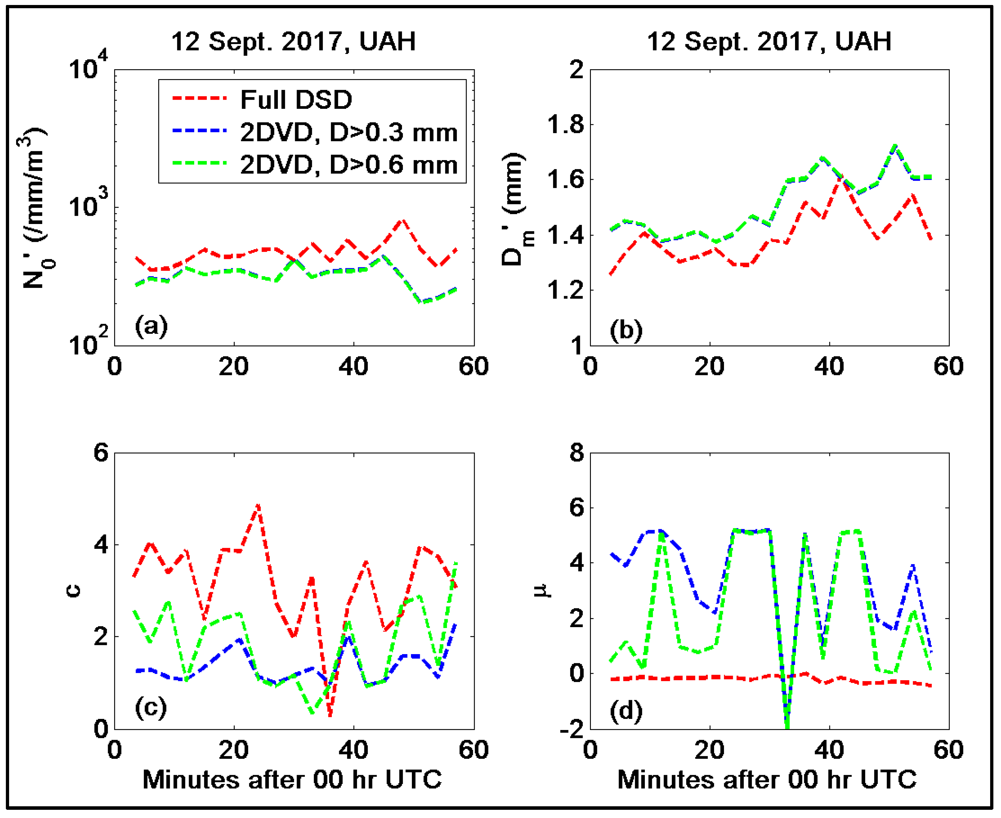
Another aspect of this study was to highlight the usefulness of adding the MPS for fitting the GG model. The set of four panels in Figure 9 shows an example to illustrate these effects. The blue and the green curves show the resulting parameters when using three-minute DSD data solely from 2DVD, taking all N(D) for D > 0.3 mm and for D > 0.6 mm, respectively. The red curve corresponds to the three-minute full DSD-based GG fits. For N₀′ and D_m’ (Panels (a) and (b)), the effects of adding the MPS data are clear; that is, N₀′ is generally increased and the D_m’ is reduced (as expected). For c and μ, the differences are even more significant. In particular, the μ values are large when the 2DVD data alone are used, indicating a convex down shape at the small drop end, compared with the full DSD spectra, which shows rather steady μ values of ≈ −0.5, indicating a concave up shape, indicating the drizzle mode. Correspondingly, the c values are smaller (typically < 2) for the fits to the 2DVD data alone (i.e., tending toward more exponential-like shape at the large drop end) relative to much larger c values (3–4) for the full DSD, which indicates a fall-off more steep than exponential. Raupach et al. [8] have already highlighted the usefulness of adding the MPS data to derive the moments M₀ to M₇ by comparing with those from the 2DVD data alone. They have shown that “the large number of small drops measured by the MPS means that the complete DSDs have larger lower-order moments than the incomplete DSDs” and that the higher-order moments, viz. M₄, M₅, M₆, and M₇, are less affected.

Finally, a GPM core satellite overpass of Huntsville that occurred during tropical storm Nate was considered. The instrument site in Huntsville sampled rainfall produced by Nate’s outer bands for more than 6 h. Comparison between the retrievals of DSD parameters from the dual-frequency precipitation radar onboard the GPM satellite and the ground-based point measurements using the MPS-2DVD composite data exhibit reasonable agreement in terms of the co-variability of the two main DSD parameters (N_w and D_m). The optimal values of µ and c for the rain bands of tropical storm Nate were found to be very close to the climatological values, thereby further consolidating the stability of h(x) across various rain types and intensities.