SXGBsite: Prediction of Protein–Ligand Binding Sites Using Sequence Information and Extreme Gradient Boosting


Abstract
1. Introduction
2. Materials and Methods
2.1. Benchmark Datasets
2.2. Feature Extraction
2.2.1. Position-Specific Scoring Matrix
2.2.2. Discrete Cosine Transform
2.2.3. Discrete Wavelet Transform
2.2.4. Predicting Solvent Accessibility
2.3. SMOTE Over-Sampling
2.4. Extreme Gradient Boosting Algorithm
3. Results
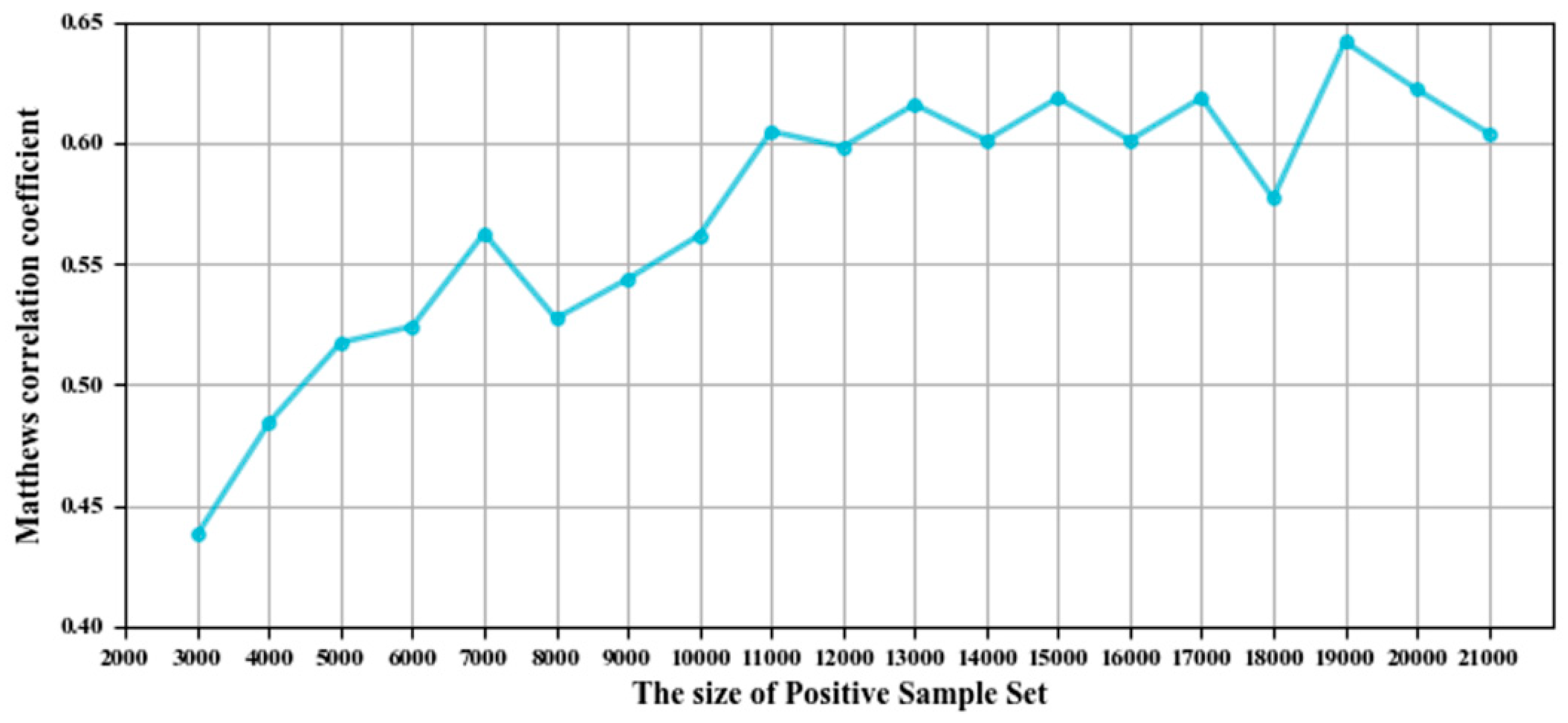
3.1. Parameter Selection
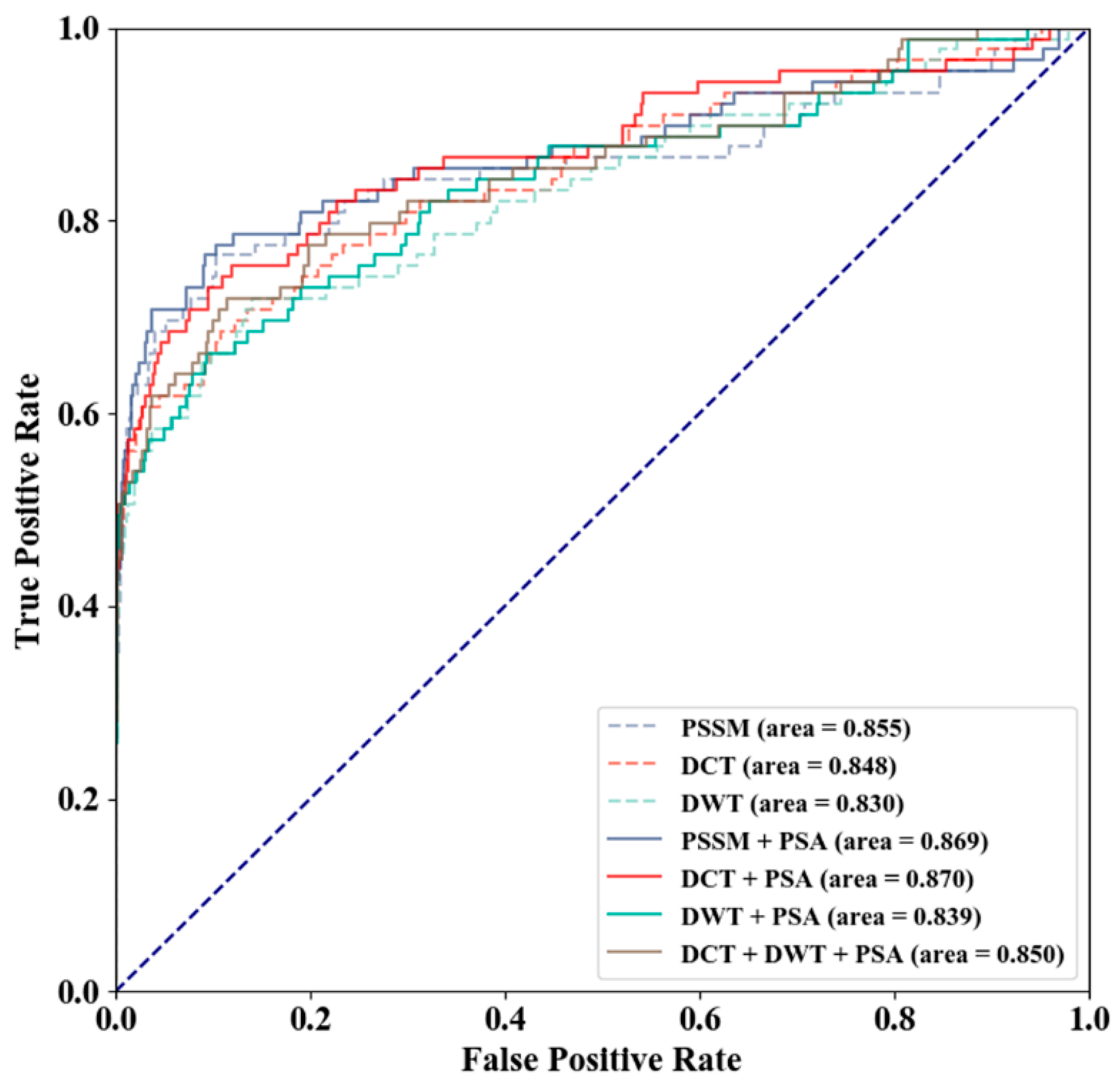
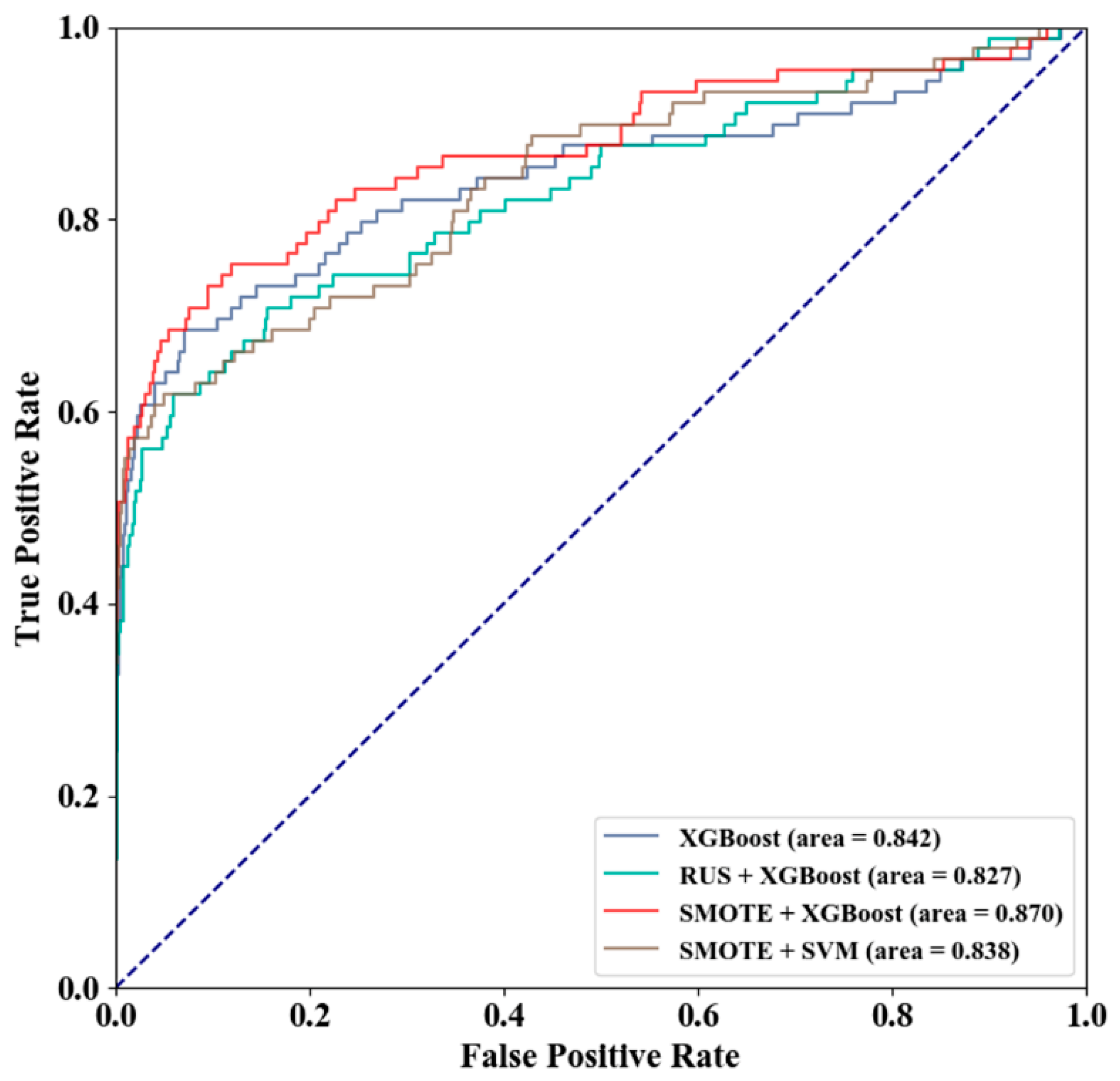
3.2. Method Selection
3.3. Results of Training Sets
3.4. Comparison with Existing Methods
3.5. Running Time Comparison
3.6. Comparison with Existing Methods on the PDNA-41 Independent Test Set
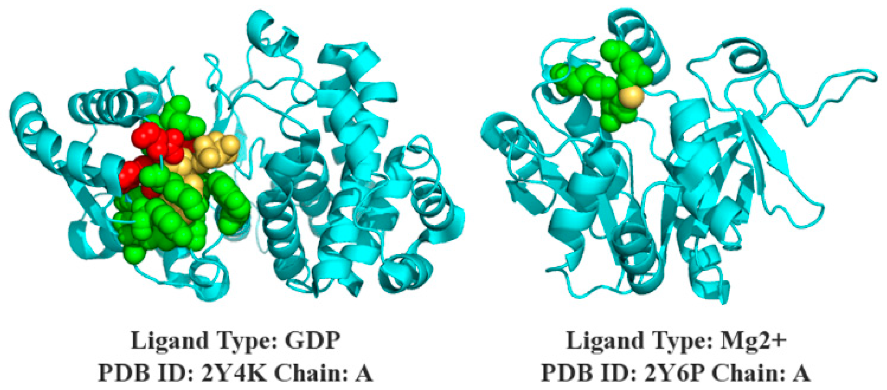
3.7. Case Study
4. Discussion
5. Conclusions
Author Contributions
Funding
Conflicts of Interest
References
- Roche, D.B.; Tetchner, S.J.; McGuffin, L.J. FunFOLD: An improved automated method for the prediction of ligand binding residues using 3D models of proteins. BMC Bioinform. 2011, 12, 160. [Google Scholar] [CrossRef]
- Hendlich, M.; Rippmann, F.; Barnickel, G. LIGSITE: Automatic and efficient detection of potential small molecule-binding sites in proteins. J. Mol. Graph. Model. 1997, 15, 359–363. [Google Scholar] [CrossRef]
- Roche, D.B.; Brackenridge, D.A.; McGuffin, L.J. Proteins and their interacting partners: An introduction to protein–ligand binding site prediction methods. Int. J. Mol. Sci. 2015, 16, 29829–29842. [Google Scholar] [CrossRef] [PubMed]
- Rose, P.W.; Prlić, A.; Bi, C.; Bluhm, W.F.; Christie, C.H.; Dutta, S.; Green, R.K.; Goodsell, D.S.; Westbrook, J.D.; Woo, J.; et al. The RCSB Protein Data Bank: Views of structural biology for basic and applied research and education. Nucleic Acids Res. 2015, 43, D345–D356. [Google Scholar] [CrossRef] [PubMed]
- Ma, X.; Guo, J.; Liu, H.D.; Xie, J.M.; Sun, X. Sequence-based prediction of DNA-binding residues in proteins with conservation and correlation information. IEEE/ACM Trans. Comput. Biol. Bioinform. 2012, 9, 1766–1775. [Google Scholar] [CrossRef]
- Ding, Y.; Tang, J.; Guo, F. Identification of protein–protein interactions via a novel matrix-based sequence representation model with amino acid contact information. Int. J. Mol. Sci. 2016, 17, 1623. [Google Scholar] [CrossRef]
- Yu, D.J.; Hu, J.; Yang, J.; Shen, H.B.; Tang, J.; Yang, J.Y. Designing template-free predictor for targeting protein-ligand binding sites with classifier ensemble and spatial clustering. IEEE/ACM Trans. Comput. Biol. Bioinform. 2013, 10, 994–1008. [Google Scholar] [CrossRef]
- Ding, Y.; Tang, J.; Guo, F. Identification of protein–ligand binding sites by sequence information and ensemble classifier. J. Chem. Inf. Model. 2017, 57, 3149–3161. [Google Scholar] [CrossRef]
- Levitt, D.G.; Banaszak, L.J. POCKET: A computer graphies method for identifying and displaying protein cavities and their surrounding amino acids. J. Mol. Graph. 1992, 10, 229–234. [Google Scholar] [CrossRef]
- Laskowski, R.A. SURFNET: A program for visualizing molecular surfaces, cavities, and intermolecular interactions. J. Mol. Graph. Model. 1995, 13, 323–330. [Google Scholar] [CrossRef]
- Xie, Z.R.; Hwang, M.J. Methods for Predicting Protein–Ligand Binding Sites. In Molecular Modeling of Proteins; Kukol, A., Ed.; Springer: New York, NY, USA, 2015; Volume 1215, pp. 383–398. [Google Scholar]
- Huang, B.; Schroeder, M. LIGSITEcsc: Predicting ligand binding sites using the Connolly surface and degree of conservation. BMC Struct. Biol. 2006, 6, 19. [Google Scholar] [CrossRef] [PubMed]
- Liang, J.; Woodward, C.; Edelsbrunner, H. Anatomy of protein pockets and cavities: Measurement of binding site geometry and implications for ligand design. Protein Sci. 1998, 7, 1884–1897. [Google Scholar] [CrossRef] [PubMed]
- Binkowski, T.A.; Naghibzadeh, S.; Liang, J. CASTp: Computed atlas of surface topography of proteins. Nucleic Acids Res. 2003, 31, 3352–3355. [Google Scholar] [CrossRef] [PubMed]
- Dundas, J.; Ouyang, Z.; Tseng, J.; Binkowski, A.; Turpaz, Y.; Liang, J. CASTp: Computed atlas of surface topography of proteins with structural and topographical mapping of functionally annotated residues. Nucleic Acids Res. 2006, 34, W116–W118. [Google Scholar] [CrossRef]
- Tian, W.; Chen, C.; Lei, X.; Zhao, J.; Liang, J. CASTp 3.0: Computed atlas of surface topography of proteins. Nucleic Acids Res. 2018, 46, W363–W367. [Google Scholar] [CrossRef]
- Fuller, J.C.; Martinez, M.; Henrich, S.; Stank, A.; Richter, S.; Wade, R.C. LigDig: A web server for querying ligand–protein interactions. Bioinformatics 2014, 31, 1147–1149. [Google Scholar] [CrossRef]
- Le Guilloux, V.; Schmidtke, P.; Tuffery, P. Fpocket: An open source platform for ligand pocket detection. BMC Bioinform. 2009, 10, 168. [Google Scholar] [CrossRef]
- Schmidtke, P.; Le Guilloux, V.; Maupetit, J.; Tuffery, P. Fpocket: Online tools for protein ensemble pocket detection and tracking. Nucleic Acids Res. 2010, 38, 582–589. [Google Scholar] [CrossRef]
- Berman, H.M.; Westbrook, J.; Feng, Z.; Gilliland, G.; Bhat, T.N.; Weissig, H.; Shindyalov, I.N.; Bourne, P.E. The protein data bank. Nucleic Acids Res. 2000, 28, 235–242. [Google Scholar] [CrossRef]
- UniProt Consortium. UniProt: A hub for protein information. Nucleic Acids Res. 2015, 43, 204–212. [Google Scholar] [CrossRef]
- Bolton, E.E.; Wang, Y.; Thiessen, P.A.; Bryant, S.H. PubChem: Integrated Platform of Small Molecules and Biological Activities. In Annual Reports in Computational Chemistry; Wheeler, R.A., Spellmeyer, D.C., Eds.; Elsevier: Amsterdam, The Netherlands, 2008; Volume 4, pp. 217–241. [Google Scholar]
- Hastings, J.; de Matos, P.; Dekker, A.; Ennis, M.; Harsha, B.; Kale, N.; Muthukrishnan, V.; Owen, G.; Turner, S.; Williams, M.; et al. The ChEBi reference database and ontology for biologically relevant chemistry: Enhancements for 2013. Nucleic Acids Res. 2013, 41, 456–463. [Google Scholar] [CrossRef] [PubMed]
- Okuda, S.; Yamada, T.; Hamajima, M.; Itoh, M.; Katayama, T.; Bork, P.; Goto, S.; Kanehisa, M. KEGG Atlas mapping for global analysis of metabolic pathways. Nucleic Acids Res. 2008, 36, 423–426. [Google Scholar] [CrossRef] [PubMed]
- Wójcikowski, M.; Ballester, P.J.; Siedlecki, P. Performance of machine-learning scoring functions in structure-based virtual screening. Sci. Rep. 2017, 7, 46710. [Google Scholar] [CrossRef]
- Wójcikowski, M.; Zielenkiewicz, P.; Siedlecki, P. Open Drug Discovery Toolkit (ODDT): A new open-source player in the drug discovery field. J. Cheminform. 2015, 7, 26. [Google Scholar] [CrossRef] [PubMed]
- Wójcikowski, M.; Zielenkiewicz, P.; Siedlecki, P. DiSCuS: An open platform for (not only) virtual screening results management. J. Chem. Inf. Model 2014, 54, 347–354. [Google Scholar] [CrossRef]
- Babor, M.; Gerzon, S.; Raveh, B.; Sobolev, V.; Edelman, M. Prediction of transition metal-binding sites from apo protein structures. Proteins 2008, 70, 208–217. [Google Scholar] [CrossRef]
- Capra, J.A.; Laskowski, R.A.; Thornton, J.M.; Singh, M.; Funkhouser, T.A. Predicting protein ligand binding sites by combining evolutionary sequence conservation and 3D structure. PLoS Comput. Biol. 2009, 5, e1000585. [Google Scholar] [CrossRef]
- Yang, J.; Roy, A.; Zhang, Y. Protein–ligand binding site recognition using complementary binding-specific substructure comparison and sequence profile alignment. Bioinformatics 2013, 29, 2588–2595. [Google Scholar] [CrossRef]
- Liu, R.; Hu, J. HemeBIND: A novel method for heme binding residue prediction by combining structural and sequence information. BMC Bioinform. 2011, 12, 207. [Google Scholar] [CrossRef]
- Si, J.; Zhang, Z.; Lin, B.; Schroeder, M.; Huang, B. MetaDBSite: A meta approach to improve protein DNA-binding sites prediction. BMC Syst. Biol. 2011, 5, S7. [Google Scholar] [CrossRef]
- Chen, K.; Mizianty, M.J.; Kurgan, L. ATPsite: Sequence-based prediction of ATP-binding residues. Proteome Sci. 2011, 9, S4. [Google Scholar] [CrossRef] [PubMed]
- Chen, K.; Mizianty, M.J.; Kurgan, L. Prediction and analysis of nucleotide-binding residues using sequence and sequence-derived structural descriptors. Bioinformatics 2011, 28, 331–341. [Google Scholar] [CrossRef] [PubMed]
- Ofran, Y.; Mysore, V.; Rost, B. Prediction of DNA-binding residues from sequence. Bioinformatics 2007, 23, i347–i353. [Google Scholar] [CrossRef] [PubMed]
- Yan, C.; Terribilini, M.; Wu, F.; Jernigan, R.L.; Dobbs, D.; Honavar, V. Predicting DNA-binding sites of proteins from amino acid sequence. BMC Bioinform. 2006, 7, 262. [Google Scholar] [CrossRef] [PubMed]
- Wang, L.; Brown, S.J. BindN: A web-based tool for efficient prediction of DNA and RNA binding sites in amino acid sequences. Nucleic Acids Res. 2006, 34, W243–W248. [Google Scholar] [CrossRef]
- Wang, L.; Yang, M.Q.; Yang, J.Y. Prediction of DNA-binding residues from protein sequence information using random forests. BMC Genom. 2009, 10, S1. [Google Scholar] [CrossRef]
- Hwang, S.; Gou, Z.; Kuznetsov, I.B. DP-Bind: A web server for sequence-based prediction of DNA-binding residues in DNA-binding proteins. Bioinformatics 2007, 23, 634–636. [Google Scholar] [CrossRef]
- Ahmad, S.; Gromiha, M.M.; Sarai, A. Analysis and prediction of DNA-binding proteins and their binding residues based on composition, sequence and structural information. Bioinformatics 2004, 20, 477–486. [Google Scholar] [CrossRef]
- Breiman, L. Random forests. Mach. Learn. 2001, 45, 5–32. [Google Scholar] [CrossRef]
- Cortes, C.; Vapnik, V. Support-vector networks. Mach. Learn. 1995, 20, 273–297. [Google Scholar] [CrossRef]
- Lu, C.Y.; Min, H.; Gui, J.; Zhu, L.; Lei, Y.K. Face recognition via weighted sparse representation. J. Vis. Commun. Image Represent. 2013, 24, 111–116. [Google Scholar] [CrossRef]
- Shen, C.; Ding, Y.; Tang, J.; Song, J.; Guo, F. Identification of DNA–protein binding sites through multi-scale local average blocks on sequence information. Molecules 2017, 22, 2079. [Google Scholar] [CrossRef] [PubMed]
- Chen, T.; Guestrin, C. Xgboost: A Scalable Tree Boosting System. In Proceedings of the 22nd Acm sigkdd International Conference on Knowledge Discovery and Data Mining, San Francisco, CA, USA, 13–17 August 2016; pp. 785–794. [Google Scholar]
- Chawla, N.V.; Bowyer, K.W.; Hall, L.O.; Kegelmeyer, W.P. SMOTE: Synthetic minority over-sampling technique. J. Artif. Intell. Res. 2002, 16, 321–357. [Google Scholar] [CrossRef]
- Ahmed, N.; Natarajan, T.; Rao, K.R. Discrete cosine transform. IEEE T. Comput. 1974, 100, 90–93. [Google Scholar] [CrossRef]
- Yu, D.J.; Hu, J.; Huang, Y.; Shen, H.B.; Qi, Y.; Tang, Z.M.; Yang, J.Y. TargetATPsite: A template-free method for ATP-binding sites prediction with residue evolution image sparse representation and classifier ensemble. J. Comput. Chem. 2013, 34, 974–985. [Google Scholar] [CrossRef] [PubMed]
- Nanni, L.; Lumini, A.; Brahnam, S. An empirical study of different approaches for protein classification. Sci. World J. 2014, 2014, 1–17. [Google Scholar] [CrossRef]
- Nanni, L.; Brahnam, S.; Lumini, A. Wavelet images and Chou′s pseudo amino acid composition for protein classification. Amino Acids 2012, 43, 657–665. [Google Scholar] [CrossRef]
- Wang, Y.; Ding, Y.; Guo, F.; Wei, L.; Tang, J. Improved detection of DNA-binding proteins via compression technology on PSSM information. PLoS ONE 2017, 12, e0185587. [Google Scholar] [CrossRef]
- Ahmad, S.; Gromiha, M.M.; Sarai, A. Real value prediction of solvent accessibility from amino acid sequence. Proteins 2003, 50, 629–635. [Google Scholar] [CrossRef]
- Yang, J.; Roy, A.; Zhang, Y. BioLiP: A semi-manually curated database for biologically relevant ligand–protein interactions. Nucleic Acids Res. 2012, 41, D1096–D1103. [Google Scholar] [CrossRef]
- Altschul, S.F.; Madden, T.L.; Schäffer, A.A.; Zhang, J.; Zhang, Z.; Miller, W.; Lipman, D.J. Gapped BLAST and PSI-BLAST: A new generation of protein database search programs. Nucleic Acids Res. 1997, 25, 3389–3402. [Google Scholar] [CrossRef] [PubMed]
- Joo, K.; Lee, S.J.; Lee, J. Sann: Solvent accessibility prediction of proteins by nearest neighbor method. Proteins 2012, 80, 1791–1797. [Google Scholar] [CrossRef] [PubMed]
- Hu, J.; He, X.; Yu, D.J.; Yang, X.B.; Yang, J.Y.; Shen, H.B. A new supervised over-sampling algorithm with application to protein-nucleotide binding residue prediction. PLoS ONE 2014, 9, e107676. [Google Scholar] [CrossRef] [PubMed]
- Friedman, J.H. Greedy function approximation: A gradient boosting machine. Ann. Stat. 2001, 29, 1189–1232. [Google Scholar] [CrossRef]
- Deng, L.; Sui, Y.; Zhang, J. XGBPRH: Prediction of Binding Hot Spots at Protein–RNA Interfaces Utilizing Extreme Gradient Boosting. Genes 2019, 10, 242. [Google Scholar] [CrossRef] [PubMed]
- Wang, H.; Liu, C.; Deng, L. Enhanced prediction of hot spots at protein-protein interfaces using extreme gradient boosting. Sci. Rep. 2018, 8, 14285. [Google Scholar] [CrossRef]
- Friedman, J.; Hastie, T.; Tibshirani, R. Additive logistic regression: A statistical view of boosting (with discussion and a rejoinder by the authors). Ann Stat 2000, 28, 337–407. [Google Scholar] [CrossRef]
- Hu, J.; Li, Y.; Zhang, M.; Yang, X.; Shen, H.B.; Yu, D.J. Predicting protein-DNA binding residues by weightedly combining sequence-based features and boosting multiple SVMs. IEEE/ACM Trans. Comput. Biol. Bioinform. 2017, 14, 1389–1398. [Google Scholar] [CrossRef]
- Chu, W.Y.; Huang, Y.F.; Huang, C.C.; Cheng, Y.S.; Huang, C.K.; Oyang, Y.J. ProteDNA: A sequence-based predictor of sequence-specific DNA-binding residues in transcription factors. Nucleic Acid Res. 2009, 37, 396–401. [Google Scholar] [CrossRef]
- Wang, L.; Huang, C.; Yang, M.Q.; Yang, J.Y. BindN+ for accurate prediction of DNA and RNA-binding residues from protein sequence features. BMC Syst. Biol. 2010, 4, 1–9. [Google Scholar] [CrossRef]
- Li, B.Q.; Feng, K.Y.; Ding, J.; Cai, Y.D. Predicting DNA-binding sites of proteins based on sequential and 3D structural information. Mol. Genet. Genom. 2014, 289, 489–499. [Google Scholar] [CrossRef] [PubMed]


| Ligand Category | Ligand Type | Training Dataset | Independent Test Dataset | Total No. Sequences | ||
|---|---|---|---|---|---|---|
| No. Sequences | (numP,numN) | No. Sequences | (numP,numN) | |||
| Nucleotide | ATP | 221 | (3021,72334) | 50 | (647,16639) | 271 |
| ADP | 296 | (3833,98740) | 47 | (686,20327) | 343 | |
| AMP | 145 | (1603,44401) | 33 | (392,10355) | 178 | |
| GDP | 82 | (1101,26244) | 14 | (194,4180) | 96 | |
| GTP | 54 | (745,21205) | 7 | (89,1868) | 61 | |
| Metal Ion | 965 | (4914,287801) | 165 | (785,53779) | 1130 | |
| 1168 | (4705,315235) | 176 | (744,47851) | 1344 | ||
| 1138 | (3860,350716) | 217 | (852,72002) | 1355 | ||
| 335 | (1496,112312) | 58 | (237,17484) | 393 | ||
| 173 | (818,50453) | 26 | (120,9092) | 199 | ||
| DNA | 335 | (6461,71320) | 52 | (973,16225) | 387 | |
| HEME | 206 | (4380,49768) | 27 | (580,8630) | 233 | |
| Feature | Threshold | SN (%) | SP (%) | ACC (%) | MCC | AUC |
|---|---|---|---|---|---|---|
| PSSM | 0.500 | 34.8 | 99.7 | 96.8 | 0.536 | 0.855 |
| 0.139 | 46.1 | 99.5 | 97.0 | 0.596 | 0.855 | |
| PSSM-DCT | 0.500 | 43.8 | 99.7 | 97.1 | 0.605 | 0.848 |
| 0.612 | 42.7 | 99.8 | 97.2 | 0.611 | 0.848 | |
| PSSM-DWT | 0.500 | 41.6 | 99.7 | 97.0 | 0.586 | 0.830 |
| 0.458 | 43.8 | 99.7 | 97.1 | 0.605 | 0.830 | |
| PSSM + PSA | 0.500 | 37.1 | 99.9 | 97.0 | 0.581 | 0.869 |
| 0.109 | 52.8 | 99.4 | 97.2 | 0.636 | 0.869 | |
| PSSM-DCT + PSA | 0.500 | 49.4 | 99.6 | 97.3 | 0.642 | 0.870 |
| 0.421 | 50.6 | 99.6 | 97.4 | 0.650 | 0.870 | |
| PSSM-DWT + PSA | 0.500 | 46.1 | 99.7 | 97.3 | 0.630 | 0.839 |
| 0.370 | 49.4 | 99.6 | 97.3 | 0.642 | 0.839 | |
| PSSM-DCT + PSSM-DWT + PSA | 0.500 | 44.9 | 99.6 | 97.1 | 0.607 | 0.850 |
| 0.545 | 44.9 | 99.8 | 97.3 | 0.629 | 0.850 |
| Scheme | Threshold | SN (%) | SP (%) | ACC (%) | MCC | AUC |
|---|---|---|---|---|---|---|
| XGBoost | 0.500 | 30.3 | 99.8 | 96.7 | 0.512 | 0.842 |
| 0.153 | 37.1 | 99.7 | 96.9 | 0.556 | 0.842 | |
| RUS + XGBoost | 0.500 | 68.5 | 84.5 | 83.8 | 0.288 | 0.827 |
| 0.914 | 51.7 | 97.9 | 95.8 | 0.504 | 0.827 | |
| SMOTE + XGBoost | 0.500 | 49.4 | 99.6 | 97.3 | 0.642 | 0.870 |
| 0.421 | 50.6 | 99.6 | 97.4 | 0.650 | 0.870 | |
| SMOTE + SVM | 0.500 | 51.7 | 99.3 | 97.1 | 0.616 | 0.838 |
| 0.714 | 49.4 | 99.5 | 97.2 | 0.628 | 0.838 |
| Ligand | Predictor | Threshold | SN (%) | SP (%) | ACC (%) | MCC | AUC |
|---|---|---|---|---|---|---|---|
| ATP | TargetS 1 | 0.500 | 48.4 | 98.2 | 96.2 | 0.492 | 0.887 |
| EC-RUS 2 | 0.500 | 84.1 | 84.9 | 84.9 | 0.347 | 0.912 | |
| 0.814 | 58.6 | 97.9 | 96.4 | 0.537 | 0.912 | ||
| SXGBsite | 0.500 | 53.4 | 96.3 | 94.6 | 0.413 | 0.886 | |
| 0.775 | 40.3 | 98.6 | 96.4 | 0.448 | 0.886 | ||
| ADP | TargetS 1 | 0.500 | 56.1 | 98.8 | 97.2 | 0.591 | 0.907 |
| EC-RUS 2 | 0.500 | 87.8 | 87.7 | 87.7 | 0.395 | 0.939 | |
| 0.852 | 62.2 | 98.6 | 97.3 | 0.610 | 0.939 | ||
| SXGBsite | 0.500 | 61.6 | 96.2 | 94.9 | 0.459 | 0.907 | |
| 0.832 | 46.4 | 98.9 | 97.0 | 0.521 | 0.907 | ||
| AMP | TargetS 1 | 0.500 | 38.0 | 98.2 | 96.0 | 0.386 | 0.856 |
| EC-RUS 2 | 0.500 | 81.5 | 79.7 | 79.8 | 0.263 | 0.888 | |
| 0.835 | 46.7 | 98.3 | 96.6 | 0.460 | 0.888 | ||
| SXGBsite | 0.500 | 37.0 | 97.8 | 95.8 | 0.347 | 0.851 | |
| 0.636 | 32.3 | 98.6 | 96.4 | 0.366 | 0.851 | ||
| GDP | TargetS 1 | 0.430 | 63.9 | 98.7 | 97.2 | 0.644 | 0.908 |
| EC-RUS 2 | 0.500 | 86.1 | 89.8 | 89.7 | 0.435 | 0.937 | |
| 0.816 | 67.2 | 98.9 | 97.6 | 0.676 | 0.937 | ||
| SXGBsite | 0.500 | 59.4 | 99.3 | 97.7 | 0.664 | 0.930 | |
| 0.653 | 57.0 | 99.5 | 97.9 | 0.678 | 0.930 | ||
| GTP | TargetS 1 | 0.500 | 48.0 | 98.7 | 96.9 | 0.506 | 0.858 |
| EC-RUS 2 | 0.500 | 79.5 | 85.7 | 85.5 | 0.309 | 0.896 | |
| 0.842 | 49.5 | 99.2 | 97.6 | 0.562 | 0.896 | ||
| SXGBsite | 0.500 | 42.4 | 99.4 | 97.6 | 0.540 | 0.883 | |
| 0.685 | 40.7 | 99.7 | 97.8 | 0.572 | 0.883 | ||
| TargetS 1 | 0.690 | 19.2 | 99.7 | 98.4 | 0.320 | 0.784 | |
| EC-RUS 2 | 0.500 | 73.9 | 73.8 | 73.8 | 0.118 | 0.812 | |
| 0.861 | 14.7 | 99.7 | 98.6 | 0.220 | 0.812 | ||
| SXGBsite | 0.500 | 32.8 | 95.0 | 94.2 | 0.135 | 0.757 | |
| 0.818 | 16.3 | 99.1 | 98.1 | 0.167 | 0.757 | ||
| TargetS 1 | 0.810 | 26.4 | 99.8 | 99.0 | 0.383 | 0.798 | |
| EC-RUS 2 | 0.500 | 73.8 | 79.4 | 79.3 | 0.125 | 0.839 | |
| 0.864 | 25.8 | 99.8 | 99.1 | 0.354 | 0.839 | ||
| SXGBsite | 0.500 | 46.1 | 95.9 | 95.5 | 0.196 | 0.819 | |
| 0.926 | 26.3 | 99.7 | 99.0 | 0.326 | 0.819 | ||
| TargetS 1 | 0.740 | 40.8 | 99.5 | 98.7 | 0.445 | 0.901 | |
| EC-RUS 2 | 0.500 | 83.4 | 86.6 | 86.6 | 0.201 | 0.921 | |
| 0.841 | 31.0 | 99.6 | 98.9 | 0.358 | 0.921 | ||
| SXGBsite | 0.500 | 45.0 | 98.3 | 97.7 | 0.297 | 0.888 | |
| 0.759 | 36.1 | 99.1 | 98.5 | 0.329 | 0.888 | ||
| TargetS 1 | 0.810 | 51.8 | 99.6 | 98.8 | 0.592 | 0.922 | |
| EC-RUS 2 | 0.500 | 87.1 | 90.1 | 90.0 | 0.278 | 0.940 | |
| 0.809 | 53.1 | 99.2 | 98.6 | 0.489 | 0.940 | ||
| SXGBsite | 0.500 | 48.2 | 99.1 | 98.5 | 0.440 | 0.913 | |
| 0.496 | 50.1 | 99.1 | 98.5 | 0.454 | 0.913 | ||
| TargetS 1 | 0.830 | 50.0 | 99.6 | 98.9 | 0.557 | 0.938 | |
| EC-RUS 2 | 0.500 | 88.7 | 90.8 | 90.8 | 0.279 | 0.958 | |
| 0.860 | 45.6 | 99.3 | 98.7 | 0.440 | 0.958 | ||
| SXGBsite | 0.500 | 59.7 | 96.5 | 96.1 | 0.299 | 0.892 | |
| 0.894 | 38.5 | 99.2 | 98.5 | 0.363 | 0.892 | ||
| DNA | TargetS 1 | 0.490 | 41.7 | 94.5 | 89.9 | 0.362 | 0.824 |
| EC-RUS 2 | 0.500 | 81.9 | 71.8 | 72.3 | 0.259 | 0.852 | |
| 0.763 | 48.7 | 95.1 | 92.6 | 0.378 | 0.852 | ||
| SXGBsite | 0.500 | 41.0 | 92.3 | 89.6 | 0.255 | 0.827 | |
| 0.420 | 49.8 | 89.2 | 87.2 | 0.270 | 0.827 | ||
| HEME | TargetS 1 | 0.650 | 50.5 | 98.3 | 94.4 | 0.579 | 0.887 |
| EC-RUS 2 | 0.500 | 85.0 | 83.6 | 83.7 | 0.416 | 0.922 | |
| 0.846 | 60.3 | 97.5 | 95.1 | 0.591 | 0.922 | ||
| SXGBsite | 0.500 | 59.3 | 96.2 | 93.8 | 0.520 | 0.900 | |
| 0.805 | 45.3 | 98.9 | 95.4 | 0.555 | 0.900 |
| Ligand | Predictor | SN (%) | SP (%) | ACC (%) | MCC | AUC |
|---|---|---|---|---|---|---|
| ATP | TargetS 1 | 50.1 | 98.3 | 96.5 | 0.502 | 0.898 |
| NsitePred 1 | 50.8 | 97.3 | 95.5 | 0.439 | - | |
| SVMPred 1 | 47.3 | 96.7 | 94.9 | 0.387 | 0.877 | |
| alignment-based 1 | 30.6 | 97.0 | 94.5 | 0.265 | - | |
| EC-RUS 2 | 45.4 | 98.8 | 96.8 | 0.506 | 0.871 | |
| SXGBsite (T = 0.500) | 54.6 | 95.7 | 94.2 | 0.397 | 0.880 | |
| SXGBsite (T = 0.718) | 43.7 | 98.5 | 96.5 | 0.463 | 0.880 | |
| ADP | TargetS 1 | 46.9 | 98.9 | 97.2 | 0.507 | 0.896 |
| NsitePred 1 | 46.2 | 97.6 | 96.0 | 0.419 | - | |
| SVMPred 1 | 46.1 | 97.2 | 95.5 | 0.382 | 0.875 | |
| alignment-based 1 | 31.8 | 97.4 | 95.1 | 0.284 | - | |
| EC-RUS 2 | 44.4 | 99.2 | 97.6 | 0.511 | 0.872 | |
| SXGBsite (T = 0.500) | 53.1 | 96.9 | 95.6 | 0.399 | 0.885 | |
| SXGBsite (T = 0.844) | 37.3 | 99.5 | 97.7 | 0.488 | 0.885 | |
| AMP | TargetS 1 | 34.2 | 98.2 | 95.9 | 0.359 | 0.830 |
| NsitePred 1 | 33.9 | 97.6 | 95.3 | 0.321 | - | |
| SVMPred 1 | 32.1 | 96.4 | 94.1 | 0.255 | 0.798 | |
| alignment-based 1 | 19.6 | 97.3 | 94.5 | 0.178 | - | |
| EC-RUS 2 | 24.9 | 99.5 | 97.0 | 0.393 | 0.815 | |
| SXGBsite (T = 0.500) | 36.0 | 97.5 | 95.4 | 0.325 | 0.823 | |
| SXGBsite (T = 0.486) | 37.1 | 97.4 | 95.3 | 0.328 | 0.823 | |
| GDP | TargetS 1 | 56.2 | 98.1 | 96.2 | 0.550 | 0.896 |
| NsitePred 1 | 55.7 | 97.9 | 96.1 | 0.536 | - | |
| SVMPred 1 | 49.5 | 97.6 | 95.4 | 0.466 | 0.870 | |
| alignment-based 1 | 41.2 | 97.8 | 95.3 | 0.415 | - | |
| EC-RUS 2 | 36.6 | 99.9 | 97.1 | 0.579 | 0.872 | |
| SXGBsite (T = 0.500) | 46.4 | 99.0 | 96.7 | 0.551 | 0.894 | |
| SXGBsite (T = 0.687) | 40.2 | 99.7 | 97.1 | 0.576 | 0.894 | |
| GTP | TargetS 1 | 57.3 | 98.8 | 96.9 | 0.617 | 0.855 |
| NsitePred 1 | 58.4 | 95.7 | 94.0 | 0.448 | - | |
| SVMPred 1 | 48.3 | 91.7 | 89.7 | 0.276 | 0.821 | |
| alignment-based 1 | 52.8 | 97.9 | 95.9 | 0.516 | - | |
| EC-RUS 2 | 61.8 | 98.7 | 97.0 | 0.641 | 0.861 | |
| SXGBsite (T = 0.500) | 49.4 | 99.6 | 97.3 | 0.642 | 0.870 | |
| SXGBsite (T = 0.421) | 50.6 | 99.6 | 97.4 | 0.650 | 0.870 |
| Ligand | Predictor | SN (%) | SP (%) | ACC (%) | MCC | AUC |
|---|---|---|---|---|---|---|
| TargetS 1 | 13.8 | 99.8 | 98.8 | 0.243 | 0.767 | |
| FunFOLD 1 | 12.2 | 99.6 | 98.1 | 0.196 | - | |
| CHED 1 | 18.7 | 98.2 | 97.1 | 0.142 | - | |
| alignment-based 1 | 20.3 | 98.6 | 97.5 | 0.175 | - | |
| EC-RUS 2 | 17.3 | 99.6 | 98.7 | 0.225 | 0.779 | |
| SXGBsite (T = 0.500) | 32.6 | 95.6 | 94.9 | 0.139 | 0.758 | |
| SXGBsite (T = 0.832) | 13.3 | 99.7 | 98.7 | 0.197 | 0.758 | |
| TargetS 1 | 18.3 | 99.8 | 98.8 | 0.294 | 0.706 | |
| FunFOLD 1 | 22.0 | 99.1 | 98.3 | 0.215 | - | |
| CHED 1 | 14.6 | 98.3 | 97.3 | 0.103 | - | |
| alignment-based 1 | 14.1 | 99.2 | 98.2 | 0.147 | - | |
| EC-RUS 2 | 20.1 | 99.8 | 99.1 | 0.317 | 0.780 | |
| SXGBsite (T = 0.500) | 41.0 | 96.3 | 95.8 | 0.177 | 0.779 | |
| SXGBsite (T = 0.917) | 19.8 | 99.8 | 99.1 | 0.291 | 0.779 | |
| TargetS 1 | 40.1 | 99.5 | 98.7 | 0.449 | 0.888 | |
| FunFOLD 1 | 23.3 | 99.8 | 98.7 | 0.376 | - | |
| CHED 1 | 35.0 | 98.1 | 97.3 | 0.253 | - | |
| alignment-based 1 | 26.6 | 99.0 | 98.0 | 0.257 | - | |
| EC-RUS 2 | 35.8 | 99.6 | 98.9 | 0.403 | 0.888 | |
| SXGBsite (T = 0.500) | 44.3 | 98.3 | 97.7 | 0.299 | 0.856 | |
| SXGBsite (T = 0.797) | 34.2 | 99.5 | 98.8 | 0.382 | 0.856 | |
| TargetS 1 | 48.3 | 99.3 | 98.7 | 0.479 | 0.945 | |
| FunFOLD 1 | 47.2 | 99.1 | 98.4 | 0.432 | - | |
| CHED 1 | 49.2 | 97.0 | 96.3 | 0.279 | - | |
| alignment-based 1 | 30.0 | 99.2 | 98.3 | 0.300 | - | |
| EC-RUS 2 | 44.3 | 99.6 | 99.0 | 0.490 | 0.936 | |
| SXGBsite (T = 0.500) | 42.5 | 99.0 | 98.3 | 0.361 | 0.891 | |
| SXGBsite (T = 0.670) | 38.7 | 99.4 | 98.7 | 0.396 | 0.891 | |
| TargetS 1 | 46.4 | 99.5 | 98.7 | 0.527 | 0.936 | |
| FunFOLD 1 | 36.5 | 99.5 | 98.6 | 0.436 | - | |
| CHED 1 | 37.9 | 98.0 | 97.1 | 0.280 | - | |
| alignment-based 1 | 29.7 | 99.0 | 98.0 | 0.297 | - | |
| EC-RUS 2 | 48.9 | 99.2 | 98.6 | 0.437 | 0.958 | |
| SXGBsite (T = 0.500) | 62.4 | 96.7 | 96.3 | 0.323 | 0.906 | |
| SXGBsite (T = 0.833) | 41.0 | 99.2 | 98.6 | 0.390 | 0.906 |
| Ligand | Predictor | SN (%) | SP (%) | ACC (%) | MCC | AUC |
|---|---|---|---|---|---|---|
| DNA | TargetS 1 | 41.3 | 96.5 | 93.3 | 0.377 | 0.836 |
| MetaDBSite 1 | 58.0 | 76.4 | 75.2 | 0.192 | - | |
| DNABR 1 | 40.7 | 87.3 | 84.6 | 0.185 | - | |
| alignment-based 1 | 26.6 | 94.3 | 90.5 | 0.190 | - | |
| EC-RUS 2 | 31.5 | 97.8 | 95.2 | 0.319 | 0.814 | |
| SXGBsite (T = 0.500) | 36.5 | 95.1 | 92.8 | 0.256 | 0.826 | |
| SXGBsite (T = 0.408) | 46.2 | 92.8 | 91.0 | 0.269 | 0.826 |
| Ligand | Predictor | SN (%) | SP (%) | ACC (%) | MCC | AUC |
|---|---|---|---|---|---|---|
| HEME | TargetS (T = 0.650) 1 | 49.8 | 99.0 | 95.9 | 0.598 | 0.907 |
| TargetS(T = 0.180) 1 | 69.3 | 90.4 | 89.1 | 0.426 | 0.907 | |
| HemeBind 1 | 86.2 | 90.7 | 90.6 | 0.537 | - | |
| alignment-based 1 | 51.4 | 97.3 | 94.4 | 0.507 | - | |
| EC-RUS (T = 0.500) 2 | 83.5 | 87.5 | 87.3 | 0.453 | 0.935 | |
| EC-RUS (T = 0.859) 2 | 55.8 | 99.0 | 96.4 | 0.640 | 0.935 | |
| SXGBsite (T = 0.500) | 61.6 | 97.7 | 95.5 | 0.600 | 0.933 | |
| SXGBsite (T = 0.700) | 52.1 | 99.0 | 96.2 | 0.618 | 0.933 |
| Dataset | SXGBsite 1 | EC-RUS (SVM) 2 | EC-RUS (WSRC) 2 | Dataset | SXGBsite 1 | EC-RUS (SVM) 2 | EC-RUS (WSRC) 2 |
|---|---|---|---|---|---|---|---|
| ATP | 134.5 | 1746.3 | 7018.4 | 273.6 | 6366.5 | 25627.2 | |
| ADP | 146.2 | 4602.8 | 10940.5 | 290.9 | 6558.6 | 31094.1 | |
| AMP | 118.5 | 647.5 | 2298.1 | 124.9 | 439.5 | 2806.8 | |
| GDP | 90.4 | 284.6 | 685.8 | 110.6 | 173.3 | 1065.9 | |
| GTP | 92.6 | 115.8 | 334.6 | 215.9 | 4284.6 | 20220.6 | |
| DNA | 131.4 | 4508.5 | 9083.6 | HEME | 104.6 | 3459.9 | 2940.5 |
| Predictor | SN (%) | SP (%) | ACC (%) | MCC | AUC |
|---|---|---|---|---|---|
| BindN 1 | 45.64 | 80.90 | 79.15 | 0.143 | - |
| ProteDNA 1 | 4.77 | 99.84 | 95.11 | 0.160 | - |
| BindN + (FPR 5%) 1 | 24.11 | 95.11 | 91.58 | 0.178 | - |
| BindN + (Spec 85%) 1 | 50.81 | 85.41 | 83.69 | 0.213 | - |
| MetaDBSite 1 | 34.20 | 93.35 | 90.41 | 0.221 | - |
| DP-Bind 1 | 61.72 | 82.43 | 81.40 | 0.241 | - |
| DNABind 1 | 70.16 | 80.28 | 79.78 | 0.264 | - |
| TargetDNA (Sen Spec) 1 | 60.22 | 85.79 | 84.52 | 0.269 | - |
| TargetDNA (FPR 5%) 1 | 45.50 | 93.27 | 90.89 | 0.300 | - |
| EC-RUS (DNA) (Sen Spec) 2 | 61.04 | 77.25 | 76.44 | 0.193 | - |
| EC-RUS (DNA) (FPR 5%) 2 | 27.25 | 97.31 | 94.58 | 0.315 | - |
| SXGBsite (Sen Spec) | 60.35 | 85.94 | 84.67 | 0.272 | 0.825 |
| SXGBsite (FPR 5%) | 35.01 | 95.01 | 92.03 | 0.265 | 0.825 |
© 2019 by the authors. Licensee MDPI, Basel, Switzerland. This article is an open access article distributed under the terms and conditions of the Creative Commons Attribution (CC BY) license (http://creativecommons.org/licenses/by/4.0/).
Share and Cite
Zhao, Z.; Xu, Y.; Zhao, Y. SXGBsite: Prediction of Protein–Ligand Binding Sites Using Sequence Information and Extreme Gradient Boosting. Genes 2019, 10, 965. https://doi.org/10.3390/genes10120965
Zhao Z, Xu Y, Zhao Y. SXGBsite: Prediction of Protein–Ligand Binding Sites Using Sequence Information and Extreme Gradient Boosting. Genes. 2019; 10(12):965. https://doi.org/10.3390/genes10120965
Chicago/Turabian StyleZhao, Ziqi, Yonghong Xu, and Yong Zhao. 2019. "SXGBsite: Prediction of Protein–Ligand Binding Sites Using Sequence Information and Extreme Gradient Boosting" Genes 10, no. 12: 965. https://doi.org/10.3390/genes10120965
APA StyleZhao, Z., Xu, Y., & Zhao, Y. (2019). SXGBsite: Prediction of Protein–Ligand Binding Sites Using Sequence Information and Extreme Gradient Boosting. Genes, 10(12), 965. https://doi.org/10.3390/genes10120965