3.1. Simulation
We evaluated the performance of all six methods (A1–A6) through extensive simulation studies. Among them, A1–A3 were developed for accommodating the interaction structures with different working correlations, while A4–A6 were only focused on the identification of main effects so the structure of the group level interaction effects were not respected. Note that there are existing studies that can also achieve the selection of main effects in longitudinal studies. For example, Wang et al. [
5] adopted the smoothly clipped absolute deviation (SCAD) penalty for conducting the selection of main effects. Since the MCP is incorporated as the baseline penalty in A1–A3, A4–A6 have thus been developed based on MCP and used as benchmark methods for comparison.
The responses were generated from the model (
2) with sample size
250 and 500. The number of time points
k was set to five. The dimensions for lipid factors
were
p = 75, 150 and 300. With
q = 3 for
, we first simulated a vector of length
n from the standard normal distribution. A group of three binary dummy variables for environmental factors could then be generated after dichotomizing the vector at the 30th and 70th percentiles. In addition, the lipids were simulated from a multivariate normal distribution with mean zero and the AR1 covariance matrix with marginal variance one and auto-correlation coefficient 0.5. We simulated the random error
from a multivariate normal distribution by assuming a zero mean vector and an AR1 covariance structure with
0.5 and 0.8. Note that when considering the interactions, the actual dimensionality was much larger than
p. For instance, given
n = 250,
p = 150, and
q = 3, the total dimension for all the main and interaction effects was 604.
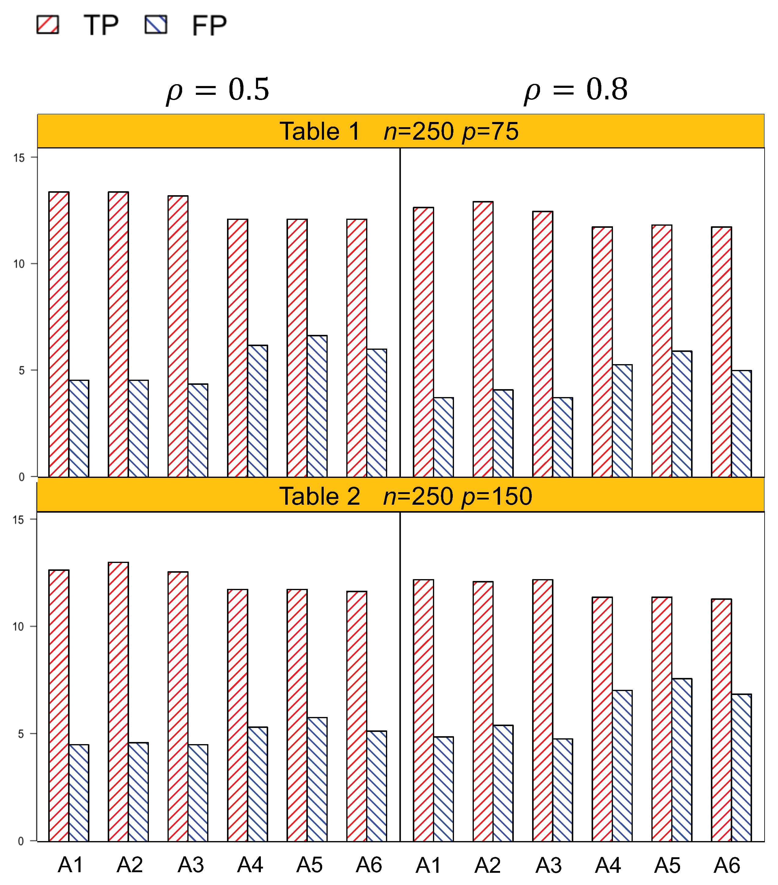
The coefficients were simulated from for 17 nonzero effects, consisting of the intercept, 3 environmental dummy variables, 4 lipid main effects, and 3 groups of lipid–environment interactions (9 interaction effects). We generated 100 replicates for the four settings: (1) n = 250 and p = 75, (2) n = 250 and p = 150, (3) n = 500 and p = 150, and (4) n = 500 and p = 300. All the rest of the coefficients were set to zero. For each setting, we considered two correlation coefficients ( 0.5 and 0.8) for the random error. The number of true positives (TP) and false positives (FP) was recorded.
In addition to identification results, we also calculated the estimation accuracy in terms of the difference between estimated and true coefficients. In particular, the mean squared error corresponding to the true nonzero coefficients and true zero coefficients (for noisy effects) were termed as MSE and NMSE, respectively. The total mean squared error for the coefficient vector, or TMSE, is computed as:
where
is the dimension of
and
is the estimated value of
in the
rth simulated dataset. MSE and NMSE were calculated in a similar way as for TMSE.
Identification results of the six methods (A1–A6) are tabulated in
Table 1,
Table 2,
Table 3 and
Table 4. In general, A1–A3, which account for both the lipid main effects and lipid–environment interactions, had better performance than A4–A6, which only accommodated the main effects. For example, in
Table 1, given
n = 250,
,
p = 75, the actual dimension is 304. A1 identified 14.5 (sd 1.9) nonzero effects out of all the 17 true positives, with a relatively small number of false positives of 4.8 (sd 3.1). On the other hand, A4 identified a smaller number of true positives, 1.3 (sd 1.5), with a larger number of false positives, 6.6 (sd 4.2). Among the identified effects, A1 identified 7.4 (sd 1.5) interactions, with 3.1 (sd 2.6) false positives. A4 identified a smaller TP of 6.1 (sd 1.1) and a higher FP of 5.1 (sd 3.3) of the lipid–environment interactions. We could observe that the difference in identification performance between A1 and A4 came mainly from the interaction effects, which was due to the fact that A4 could not accommodate the group level selection corresponding to the lipid–environment interactions. As the dimension increased, A1 outperformed A4 more significantly. For instance, in
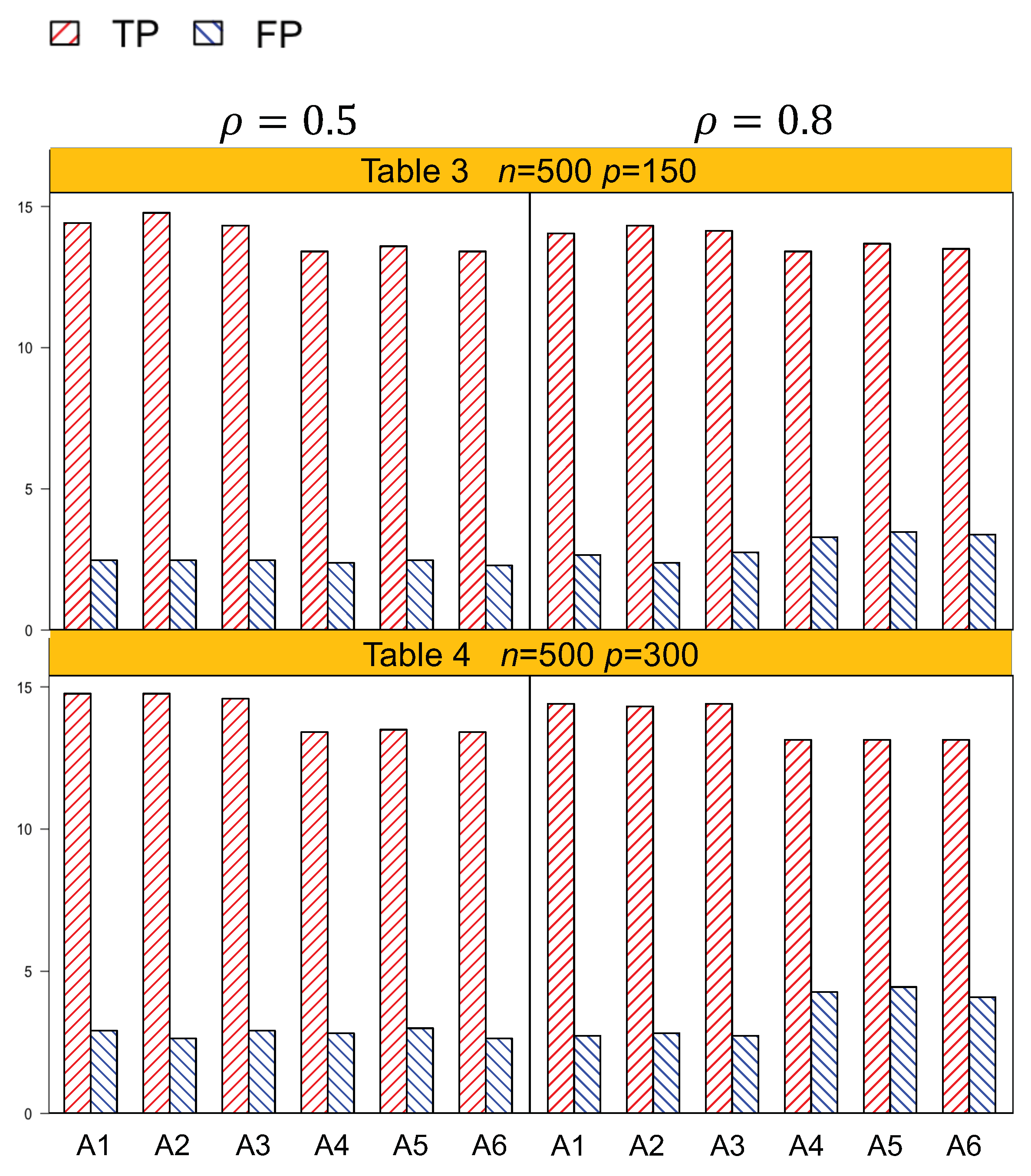
Table 4, the overall dimension for
n = 500,
,
p = 300 is 1204. A1 had a TP of 15.9 (sd 1.2) and an FP of 3 (sd 2.6), while A4 had a smaller TP 14.5 (sd 1.2) and a higher FP 4.5 (sd 3.0).
Figure 1 and
Figure 2 are plotted based on the identification results from
Table 1,
Table 2,
Table 3 and
Table 4. We can observe that overall, A1–A3 outperformed A4–A6 with a higher TP and a lower FP under each setting.
In terms of estimation accuracy, A1–A3 also had a better performance compared with A4–A4, as shown in
Table 5 and
Table 6. For the panel corresponding to
n = 250,
, and
p = 75 in
Table 5, the mean squared error for the nonzero coefficients of A1 was 0.1055, which was less than half of that of A4 (0.2321). Besides, A1 also had a smaller total mean squared error (TMSE). All the pieces of evidence suggested that A1 had higher estimation accuracy than A4. We can observe the pattern for the rest of the four methods. As the dimension increased to
n = 500,
, and
p = 300 (so the total dimension was 1204) in
Table 6, the MSE of A1 (0.0688) was also smaller than that of A4 (0.1949). There were no obvious differences in NMSE among these settings.
Another important conclusion we make from the simulation study is that, for the methods that differ only in working correlation, i.e., A1 (exchangeable), A2 (AR1), and A3 (independence), there was no significant difference in terms of either identification or estimation accuracy, as shown by
Table 1,
Table 2,
Table 3,
Table 4,
Table 5 and
Table 6, as well as
Figure 1 and
Figure 2. Such an observation suggests that the proposed methods under the GEE framework were robust to the misspecification of the working correlation, and this is consistent with the conclusions from main effects only models in longitudinal studies [
7].
To mimic the sample size and number of lipid factors in the case study, we also conducted a simulation in settings with
n = 60,
p = 30, and
q = 3. Therefore, the overall dimension of main and interaction effects was 124. The coefficients were generated from
U[1.4,1.8] for 17 nonzero effects. The identification and prediction results are summarized in
Table A1 and
Table A2 in the
Appendix A, respectively. Consistent patterns were observed. For example, in terms of identification, under
= 0.5, A1 had a higher TP of 13.6 (sd 2.5) compared to the 11.1 (sd 2.6) of A4, and a lower FP of 4.7 (sd 2.7), compared to the FP of 5.4 (sd 2.8) identified by A4.
Evaluation of all the methods, especially A1–A3, was also conducted when the true underlying model was misspecified. We generated the response (phenotype) from a main effect only model with eight true main effects when
n = 250,
p = 75,
with a total dimension of 304. Results are provided in
Table A3. When the interaction effects did not exist, A1 had only identified a very small number of false interaction effects, with 0.7 (sd 1.7) false positives. A2–A6 performed similarly in terms of identifying false interaction effects. All six methods identified a comparable number of true main effects. Overall, all methods had similar performance in identification, as well as prediction, when the data generating model had only main effects. Such a phenomenon is reasonable by further examining the results in
Table 1. We found that the major difference between A1–A3 and A4–A6 was due to the identification of interaction effects. Therefore, when only main effects were present, all the methods had comparable performances.
Penalized regression and hypothesis testing are two related, but distinct aspects in statistical analysis. The proposed study was not aimed at developing test statistics, computing the power functions, and assessing the control of type 1 error, so these statistical test related results are not available, just like most of the studies on penalized regression. Recently, efforts devoted to bridging the two areas have been mainly restricted to linear models under high-dimensional settings [
24,
25,
26]. Extensions to interaction models have not been reported so far. In particular, we are not aware of results reported for longitudinal models. Nevertheless, we conducted the simulation by assuming the null model and tabulate the identification results in
Table A4. The results should be interpreted as identification with misspecified models. As we observed, under the null model, all six methods led to a very small number of false positives.
To assess the consistency of variable selection in longitudinal settings, we carried out the stability selection [
27] under
n = 250,
p = 75, and
= 0.8. Each time, we selected 200 out of the total of 250 subjects without replacement and then conducted selection. The process was repeated 100 times, which yielded a proportion of selected effects. Larger proportions of being selected suggested stable results. Stability selection is well known for assessing the stability of penalized selection, and it alleviates the concern that the effects have only been identified by chance. We investigate the selection proportions of the 17 true main and interaction effects for all six methods in
Table A5. A1 identified 14 true effects with proportions above 70%, which is consistent with the results shown in the lower panel of
Table 1, where 13.7 TPs (sd 2.3) were identified. Such a consistent pattern can be observed across all six methods.
Although no consensus on the optimal criterion of selecting tuning parameters has been reached so far, cross-validation is perhaps the most well accepted criterion to select tuning parameters in the community of high-dimensional data analysis [
3,
4]. To further justify its appropriateness, under the setting of
n = 250 and
p = 75, we performed the analysis by selecting tuning parameters using an independently generated testing dataset with a sample size of 1000 and
p = 75. The models were fitted on the training dataset, and prediction was assessed based on the independently generated testing dataset, so no data were used in training the model. The identification and prediction results are tabulated in
Table A6 and
Table A7, respectively. A comparison to
Table 1 and
Table 5 demonstrates that the results obtained by cross-validation and validation were very close.
3.2. Real Data Analysis
We applied the proposed and alternative methods on a dataset from one of our previous studies in animal models [
15]. In the study, 60 female CD-1 mice were assigned to four different treatment groups, which were control (ad libitum feeding and sedentary), AE (exercise and ad libitum feeding), PE (exercise and pair feeding), and DCR (sedentary and 20% dietary calorie restriction). The phenotype of interest was mice’s body weight, which was measured every week for 10 weeks. Mice were sedentary and given ad libitum feeding in the control group, where they could eat as much as they wanted without doing treadmill exercises. In the AE group, mice received ad libitum feeding and ran on the treadmill every day at a speed of 0.5 mph, 1 h per day, and 5 days a week, while mice in the PE group did the same exercise, but were given the same amount of diet as the mice in the control group. Mice in the DCR group had 20% less calorie intake than the control group, but they had the same intake of protein, vitamins, and minerals. The composition of 176 plasma neutral lipid species of interest was measured. In the current study, we only focused on diacylglycerols. In addition, the diacylglycerol lipid species that have a majority of samples lower than the detection limits were excluded so there were 31 diacylglycerols. In total, there were 31 lipid main effects and 93 lipid–environment interactions.
Using the method A1 (interep with the exchangeable working correlation) as shown in
Table 7, we identified seven lipid species that had different effects in weight control of mice (AE, PE, or DCR) on body weight compared to those of the control mice. Among them, C20:1/16:1 and C20:1/20:4 had negative interactions in AE mice, where C denotes carbon. For the lipid species of C20:1/16:1,
, the regression coefficient was −2.9145 for AE mice. That is, mice with an increased amount of C20:1/16:1 tended to have a lower body weight compared to that of the control. In the AE mice, both C16:0/C16:0 and C22:6/C18:1 had strong positive associations with body weights. It is interesting that C16:0/C16:0 were negatively associated with body weight in both PE and DCR mice. C16:0 is also called palmitic acid and is one of most common saturated fatty acids. Increased consumption of palmitic acid is associated with higher risk of cardiovascular disease, type 2 diabetes, and cancer [
28]. The negative association of C16:0/16:0 and body weight in DCR and PE suggests that when the calories of the diet are restricted, the accumulation of saturated fat in the body actually decreased compared to the control. Another lipid that is negatively associated with body weight in DCR and PE mice is C18:1/16:1. The lipids that were positively associated with body weight in PE were C18:2/C16:1, C20:1/C16:1, and C22:6/C18:1. All species contain unsaturated fatty acids. Among them, C22:6 is one of the omega-3 polyunsaturated fatty acids (PUFA). In DCR, the two lipids that were positively associated with body weight were C18:2/16:1 and C20:1/20:4. Both fatty acids C18:2 and C20:4 were PUFA. The results seem to be consistent with our previous finding that exercise with paired feeding may increase the amount of PUFA in phospholipids in mice skin [
29].
In addition, we adopted A4 to analyze the lipid data. A4 also had the exchangeable working correlation, but it could not conduct group level selection of the lipid–environment interactions. The identification results are tabulated in
Table 8. Note that the selection of interactions with individual dummy environment factors was not consistent with the formulation of the lipid–environment interactions. In terms of prediction, A1 had a smaller prediction error (4.04) than that of A4 (4.97).


