
Deciphering the Genetic Architecture of Plant Virus Resistance by GWAS, State of the Art and Potential Advances

 , , and
Abstract
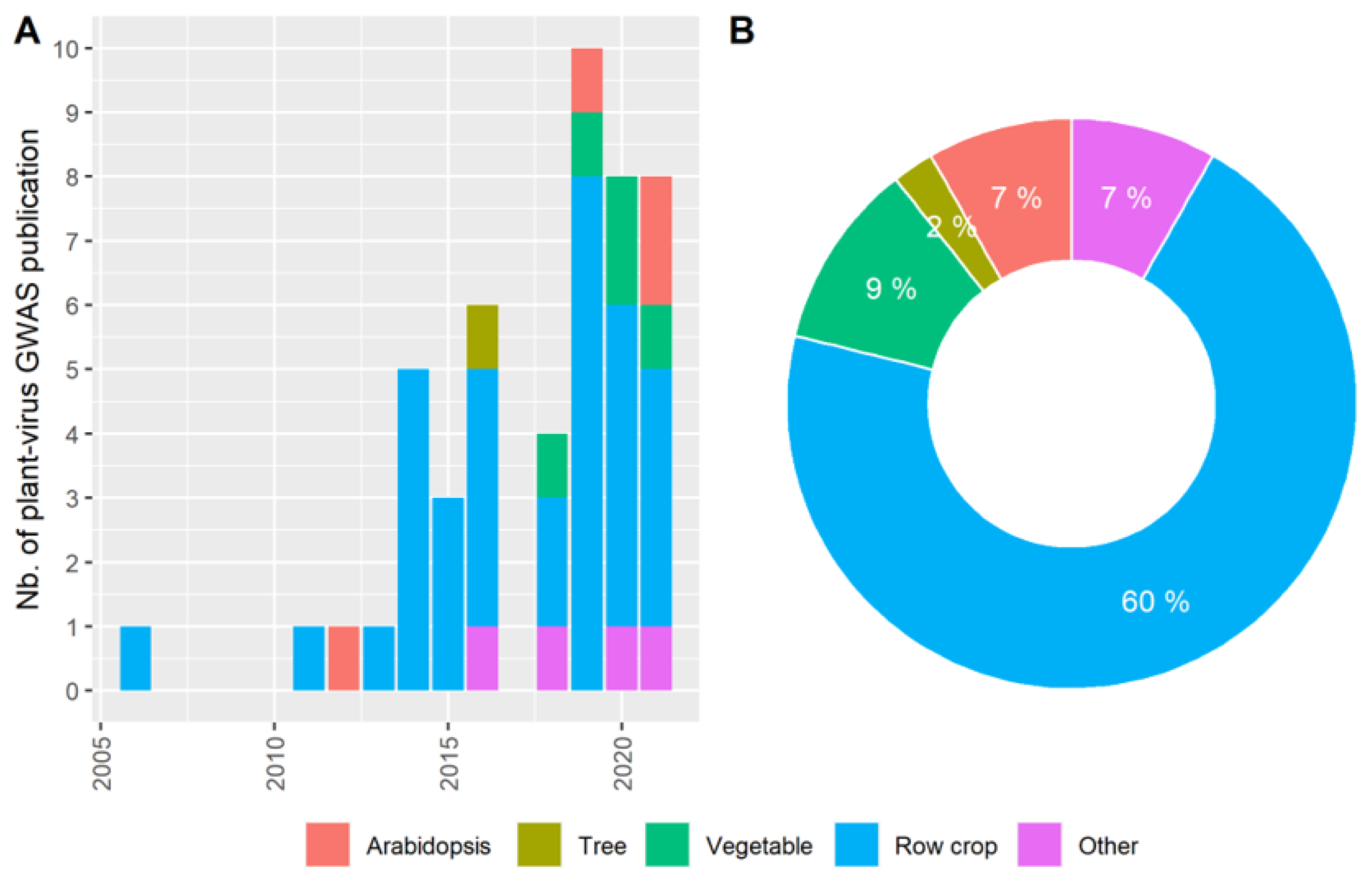
:1. Introduction
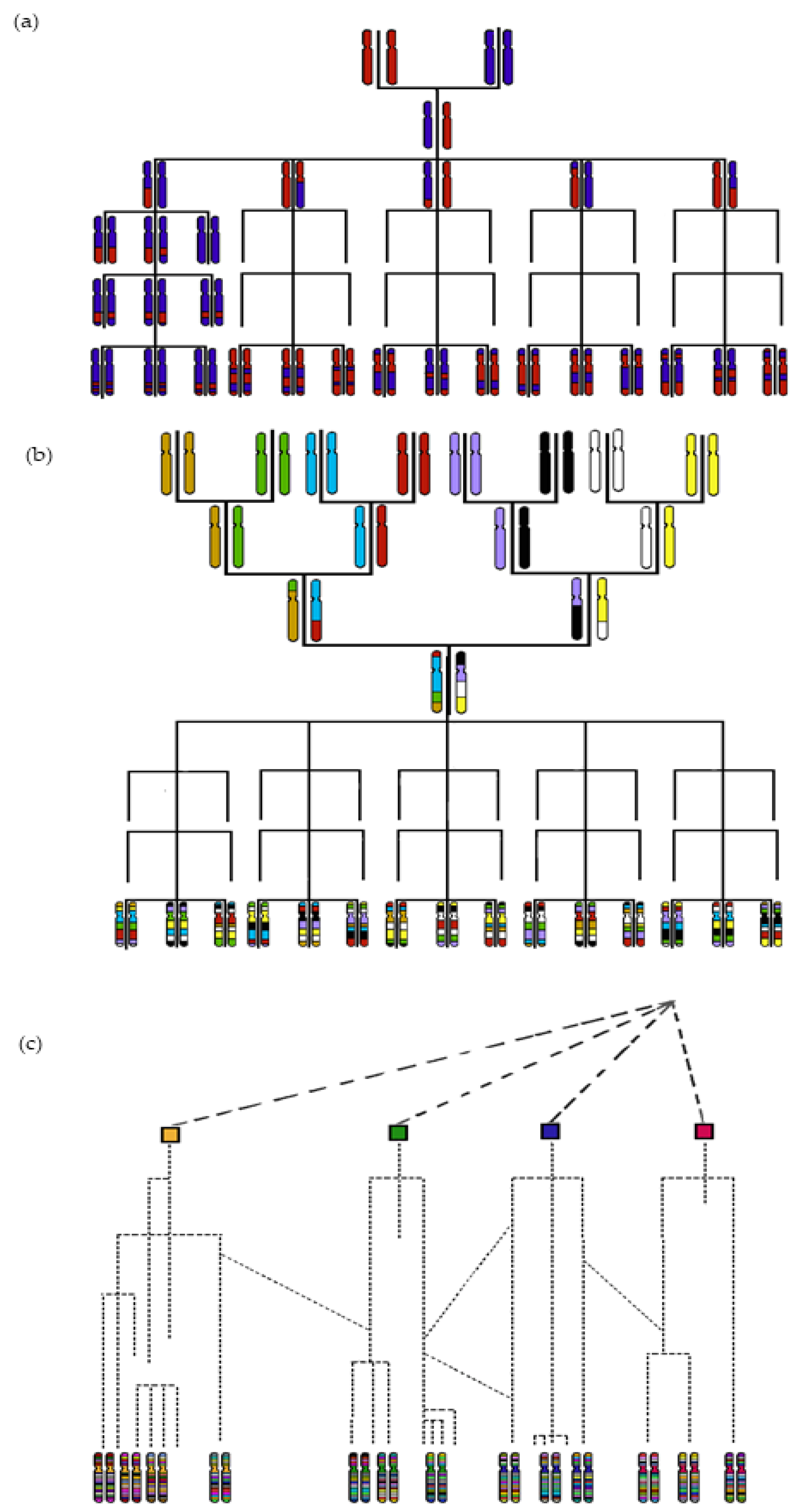
2. Mapping QTLs via GWAS Using Historical Recombinations
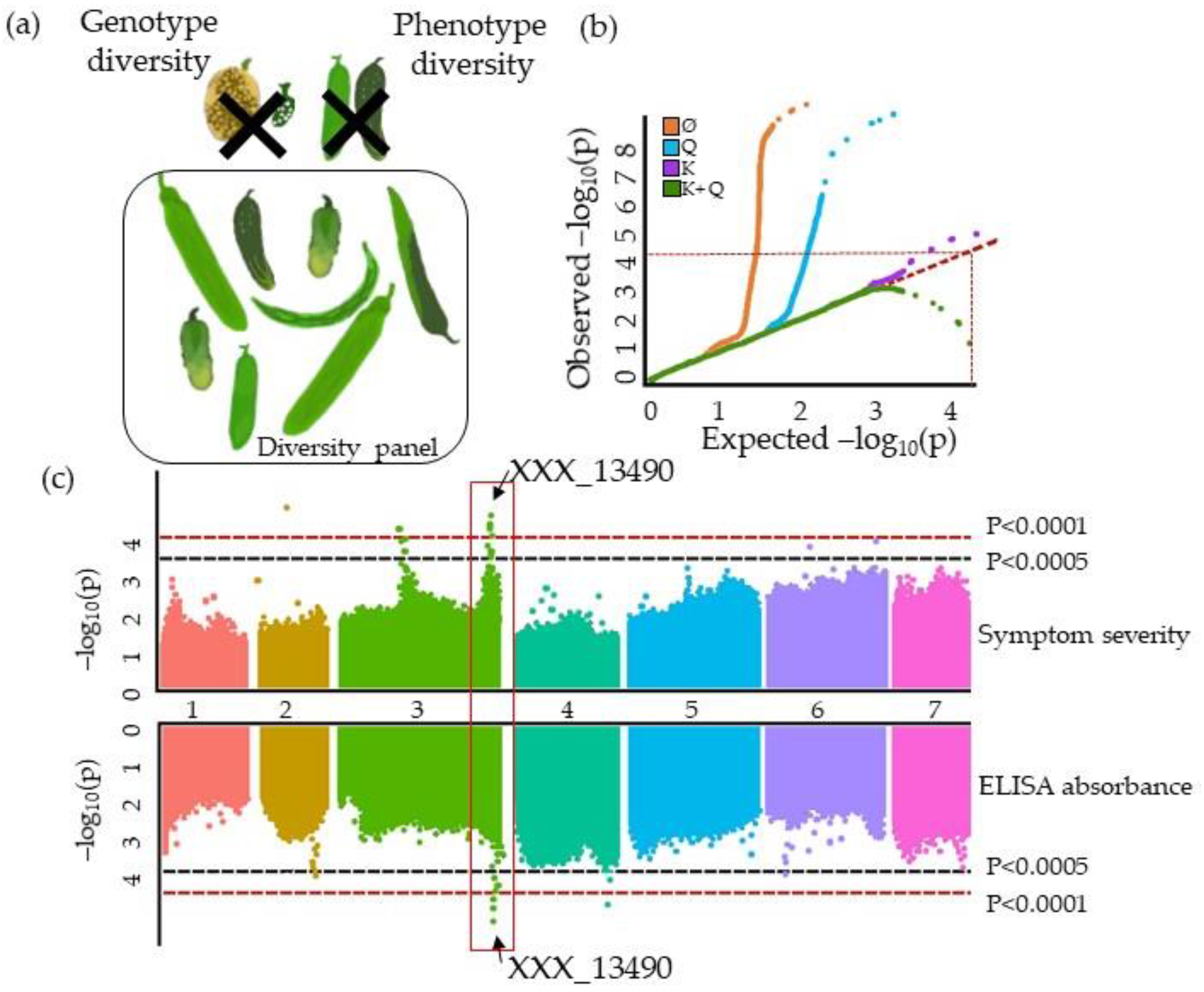
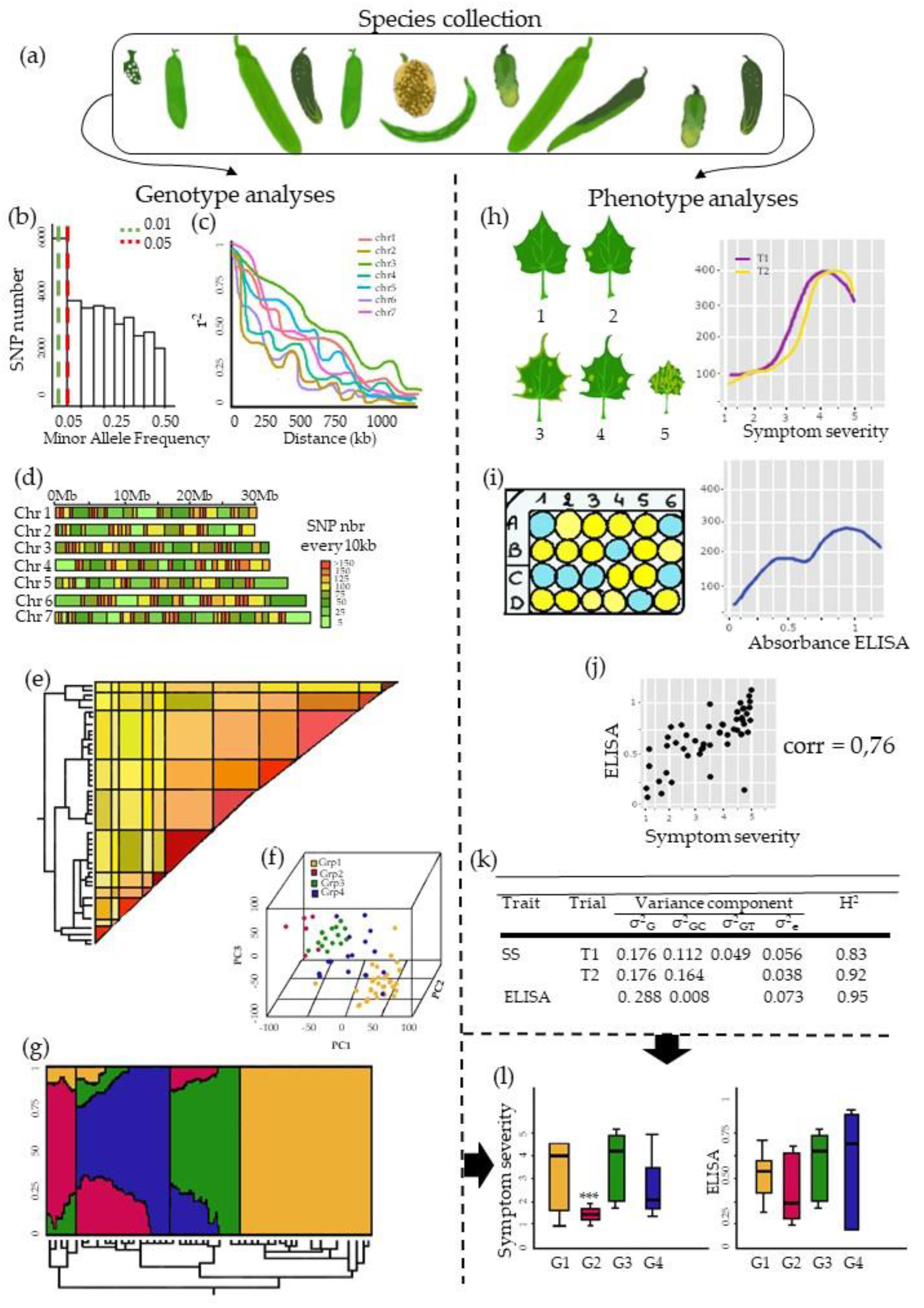
3. The Pre-GWAS Step: Assembled Diversity Panel That Is Genetically and Phenotypically Diverse
3.1. The GWAS Panel Composition Plays a Major Role in GWAS
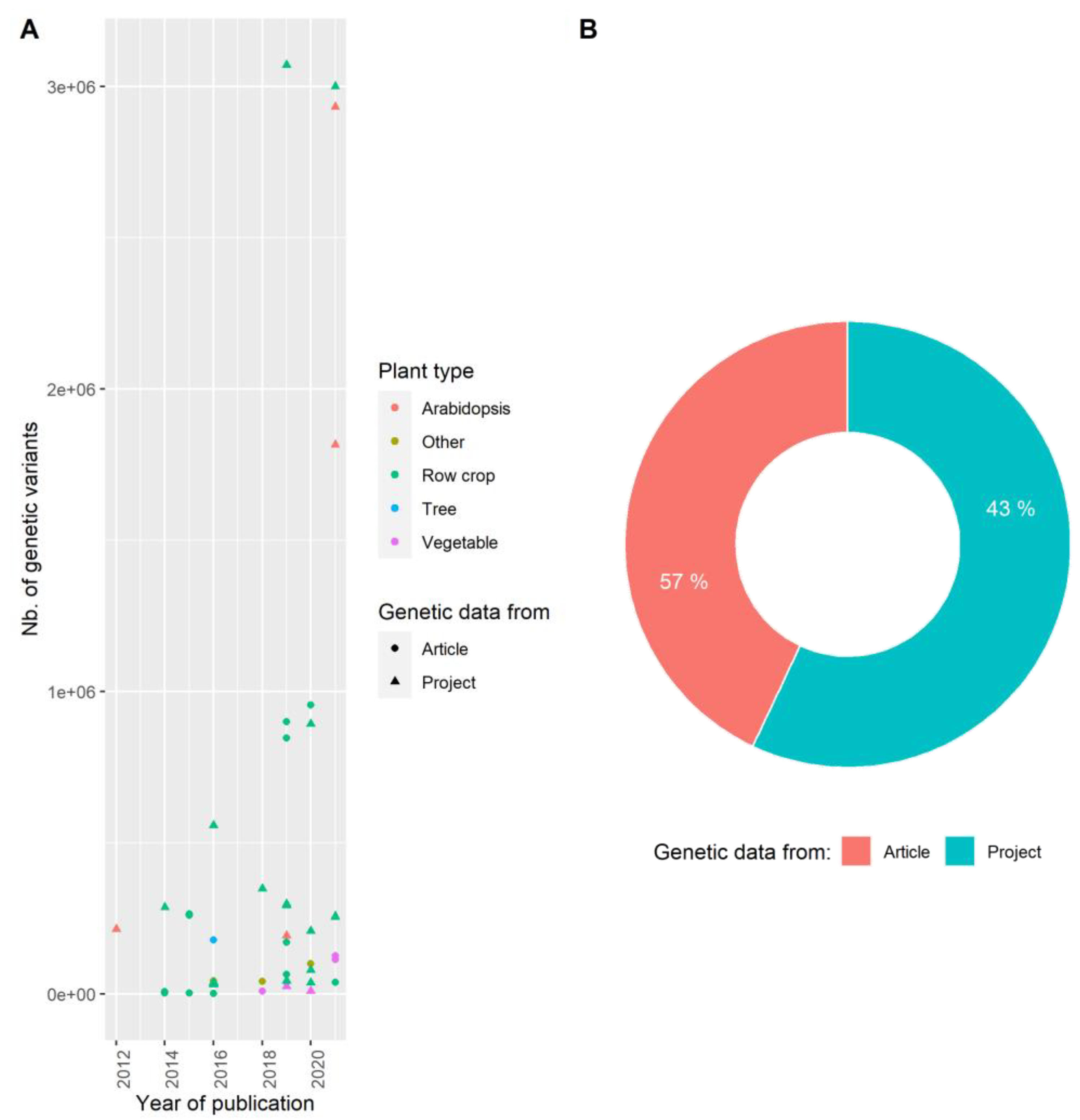
3.2. Producing Genetic Variant Array to Enhance Positive Association Detection: A New Deal for GWAS
3.3. Examining Resistance Distributions among Genetic Groups of the Panel
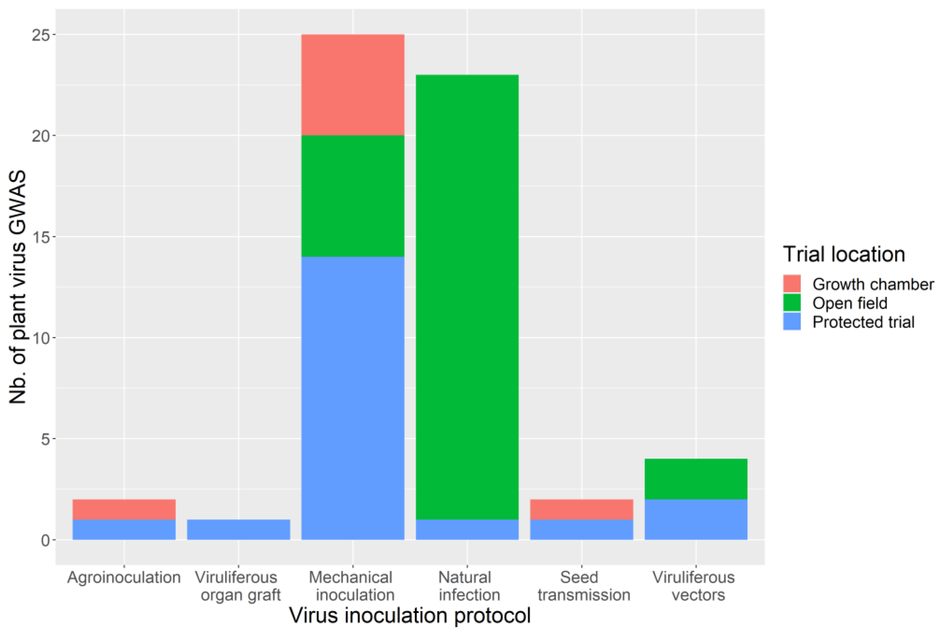
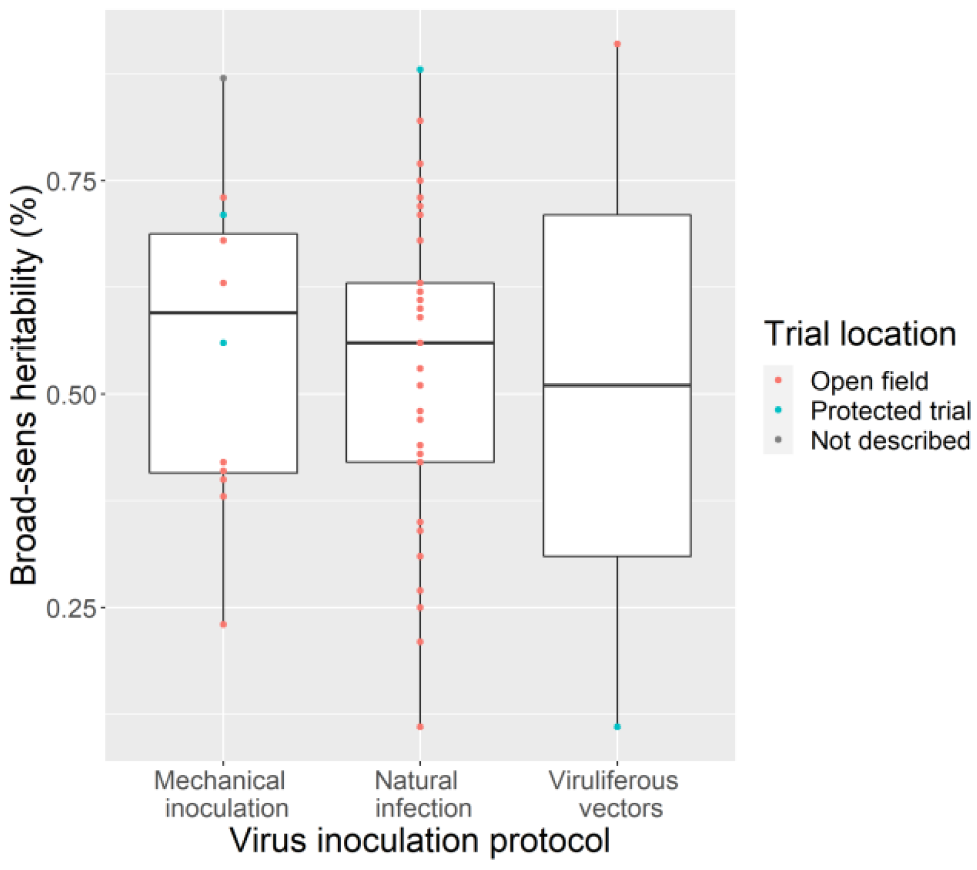
3.4. Phenotyping: Tricky Steps for a Powerful GWAS
4. The GWAS Step: Choosing a Model Tailored for the Datasets
4.1. Linear Mixed Models (LMM) Are the Most Used in GWAS
4.2. Multilocus Models in GWAS: Detecting Markers Hidden by Major Effect QTLs
4.3. Other Models That Are More Tailored to Virus Phenotype Distributions
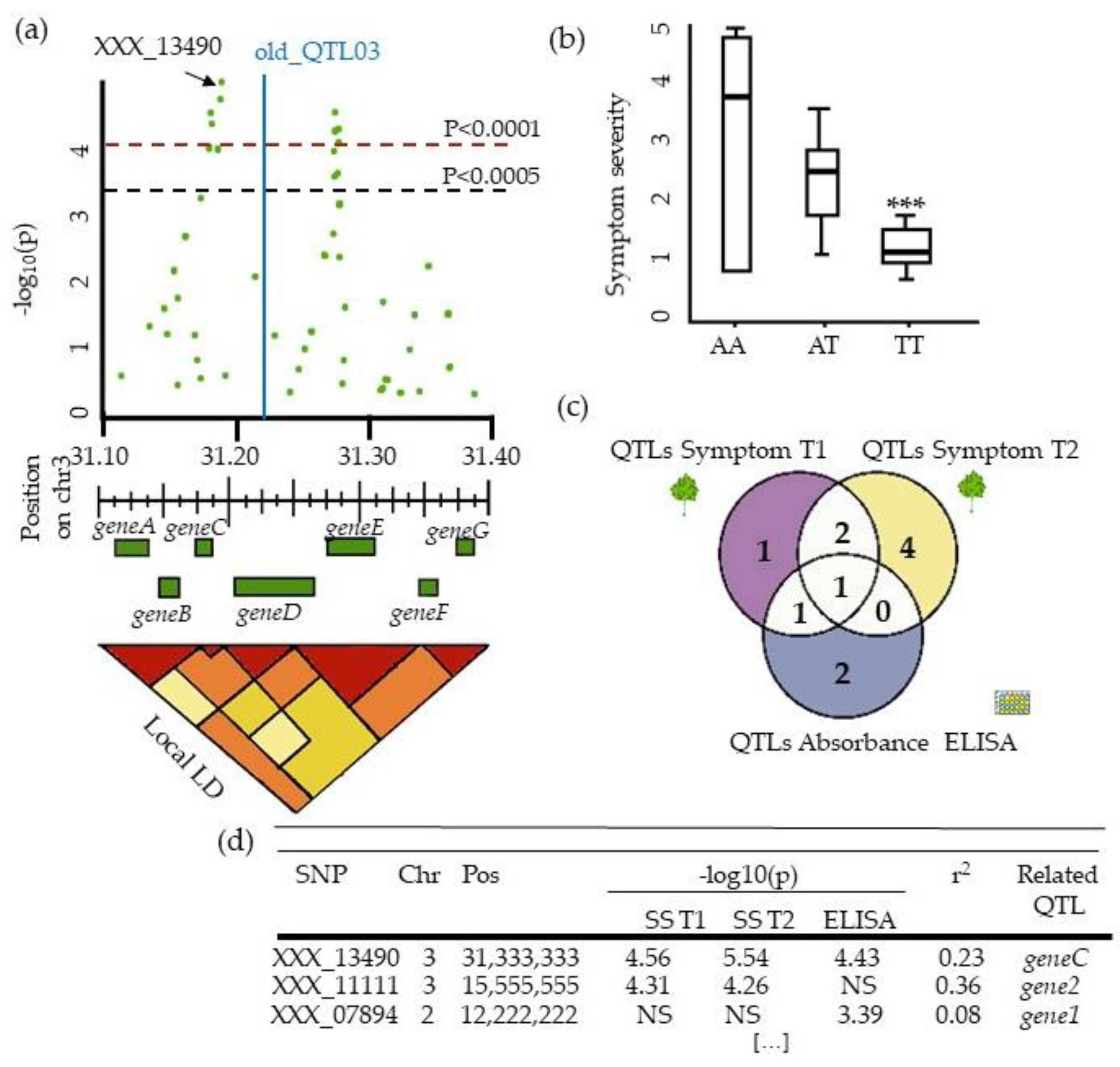
4.4. Describing QTLs: Significance, Number, Precision, and Allele Frequency
5. The Post-GWAS Step: From QTL Validation for Breeding to Candidate Gene Research
5.1. Inferring QTL Effects and Identifying Favorable Alleles… A Complex Issue
5.2. Inviting QTLs in Breeding Programs
5.3. From QTLs to Causal Genes, a Budding Approach
6. Conclusions
Supplementary Materials
Author Contributions
Funding
Institutional Review Board Statement
Informed Consent Statement
Data Availability Statement
Acknowledgments
Conflicts of Interest
References
- Anderson, P.K.; Cunningham, A.A.; Patel, N.G.; Morales, F.J.; Epstein, P.R.; Daszak, P. Emerging Infectious Diseases of Plants: Pathogen Pollution, Climate Change and Agrotechnology Drivers. Trends Ecol. Evol. 2004, 19, 535–544. [Google Scholar] [CrossRef]
- Chauhan, P.; Singla, K.; Rajbhar, M.; Singh, A.; Das, N.; Kumar, K. A Systematic Review of Conventional and Advanced Approaches for the Control of Plant Viruses. J. Appl. Biol. Biotechnol. 2019, 7, 89–98. [Google Scholar] [CrossRef]
- France: France’s Sugar Beet Crop Devastated by Disease-Sugar Industry’s Viability Threatened; U.S. Department of Agriculture, Foreign Agricultural Service, 2020.
- Martín-Hernández, A.M.; Picó, B. Natural Resistances to Viruses in Cucurbits. Agronomy 2021, 11, 23. [Google Scholar] [CrossRef]
- Hao, D.; Cheng, Y.; Chen, G.; Lu, H.; Shi, M.; Zhang, Z.; Huang, X.; Mao, Y.; Xue, L. Identification of Significant Single Nucleotide Polymorphisms for Resistance to Maize Rough Dwarf Disease in Elite Maize (Zea Mays L.) Inbred Lines. Euphytica 2015, 203, 109–120. [Google Scholar] [CrossRef]
- Feng, Z.; Kang, H.; Li, M.; Zou, L.; Wang, X.; Zhao, J.; Wei, L.; Zhou, N.; Li, Q.; Lan, Y.; et al. Identification of New Rice Cultivars and Resistance Loci against Rice Black-Streaked Dwarf Virus Disease through Genome-Wide Association Study. Rice 2019, 12, 49. [Google Scholar] [CrossRef] [PubMed] [Green Version]
- Fuchs, M.; Chirco, E.M.; Gonsalves, D. Movement of Coat Protein Genes from a Commercial Virus-Resistant Transgenic Squash into a Wild Relative. Environ. Biosaf. Res. 2004, 3, 5–16. [Google Scholar] [CrossRef] [Green Version]
- Gonsalves, D.; Gonsalves, C.; Ferreira, S.; Pitz, K.; Fitch, M.; Manshardt, R.; Slightom, J. Transgenic Virus Resistant Papaya: From Hope to Reality for Controlling Papaya Ringspot Virus in Hawaii. APSnet Features 2004. [Google Scholar] [CrossRef]
- Zamir, D. Improving plant breeding with exotic genetic libraries. Nat. Rev. Genet. 2001, 2, 983–989. [Google Scholar] [CrossRef]
- Lebeda, A.; Křístková, E.; Kitner, M.; Mieslerová, B.; Jemelková, M.; Pink, D.A.C. Wild Lactuca Species, Their Genetic Diversity, Resistance to Diseases and Pests, and Exploitation in Lettuce Breeding. Eur. J. Plant Pathol. 2014, 138, 597–640. [Google Scholar] [CrossRef]
- Chen, J.-F.; Staub, J.E.; Tashiro, Y.; Isshiki, S.; Miyazaki, S. Successful Interspecific Hybridization between Cucumis sativus L. and C. Hystrix Chakr. Euphytica 1997, 96, 413–419. [Google Scholar] [CrossRef]
- Bedinger, P.A.; Chetelat, R.T.; McClure, B.; Moyle, L.C.; Rose, J.K.C.; Stack, S.M.; van der Knaap, E.; Baek, Y.S.; Lopez-Casado, G.; Covey, P.A.; et al. Interspecific Reproductive Barriers in the Tomato Clade: Opportunities to Decipher Mechanisms of Reproductive Isolation. Sex. Plant Reprod. 2011, 24, 171–187. [Google Scholar] [CrossRef]
- Boissot, N.; Urbino, C.; Dintinger, J.; Pavis, C. Vector and Graft Inoculations of Potato Yellow Mosaic Virus Reveal Recessive Resistance in Solanum Pimpinellifolium. Ann. Appl. Biol. 2008, 152, 263–269. [Google Scholar] [CrossRef]
- Schoeny, A.; Desbiez, C.; Millot, P.; Wipf-Scheibel, C.; Nozeran, K.; Gognalons, P.; Lecoq, H.; Boissot, N. Impact of Vat Resistance in Melon on Viral Epidemics and Genetic Structure of Virus Populations. Virus Res. 2017, 241, 105–115. [Google Scholar] [CrossRef] [PubMed] [Green Version]
- Wang, Y.; Lee, K.C.; Gaba, V.; Wong, S.M.; Palukaitis, P.; Gal-On, A. Breakage of resistance to Cucumber mosaic virus by co-infection with Zucchini yellow mosaic virus: Enhancement of CMV accumulation independent of symptom expression. Arch. Virol. 2004, 149, 379–396. [Google Scholar] [CrossRef] [PubMed]
- Palloix, A.; Ayme, V.; Moury, B. Durability of Plant Major Resistance Genes to Pathogens Depends on the Genetic Background, Experimental Evidence and Consequences for Breeding Strategies. New Phytol. 2009, 183, 190–199. [Google Scholar] [CrossRef]
- Schneider, D.J.; Collmer, A. Studying Plant-Pathogen Interactions in the Genomics Era: Beyond Molecular Koch’s Postulates to Systems Biology. Annu. Rev. Phytopathol. 2010, 48, 457–479. [Google Scholar] [CrossRef] [Green Version]
- Sun, X.; Fernando, R.; Dekkers, J. Contributions of Linkage Disequilibrium and Co-Segregation Information to the Accuracy of Genomic Prediction. Genet. Sel. Evol. 2016, 48, 77. [Google Scholar] [CrossRef] [PubMed] [Green Version]
- Michelmore, R.W.; Paran, I.; Kesseli, R.V. Identification of markers linked to disease-resistance genes by bulked segregant analysis: A rapid method to detect markers in specific genomic regions by using segregating populations. Proc. Natl. Acad. Sci. USA 1991, 88, 9828–9832. [Google Scholar] [CrossRef] [Green Version]
- Gmitter, F.; Xiao, S.; Huang, S.; Hu, X.; Garnsey, S.; Deng, Z. A localized linkage map of the citrus tristeza virus resistance gene region. Theor. Appl. Genet. 1996, 92, 688–695. [Google Scholar] [CrossRef]
- Strausbaugh, C.; Myers, J.; Forster, R.; McClean, P. Bc-1 and Bc-u—Two Loci Controlling Bean Common Mosaic Virus Resistance in Common Bean Are Linked. J. Am. Soc. Hortic. Sci. 1999, 124, 644–648. [Google Scholar] [CrossRef] [Green Version]
- Ramírez-Madera, A.O.; Havey, M.J. Different Haplotypes Encode the Same Protein for Independent Sources of Zucchini Yellow Mosaic Virus Resistance in Cucumber. Hortscience 2017, 52, 1040–1042. [Google Scholar] [CrossRef] [Green Version]
- Kover, P.X.; Valdar, W.; Trakalo, J.; Scarcelli, N.; Ehrenreich, I.M.; Purugganan, M.D.; Durrant, C.; Mott, R. A Multiparent Advanced Generation Inter-Cross to Fine-Map Quantitative Traits in Arabidopsis Thaliana. PLoS Genet. 2009, 5, e1000551. [Google Scholar] [CrossRef] [PubMed] [Green Version]
- Poque, S.; Pagny, G.; Ouibrahim, L.; Chague, A.; Eyquard, J.-P.; Caballero, M.; Candresse, T.; Caranta, C.; Mariette, S.; Decroocq, V. Allelic Variation at the Rpv1 Locus Controls Partial Resistance to Plum Pox Virus Infection in Arabidopsis Thaliana. BMC Plant Biol. 2015, 15, 159. [Google Scholar] [CrossRef] [Green Version]
- Weigel, D. Natural Variation in Arabidopsis: From Molecular Genetics to Ecological Genomics. Plant Physiol. 2012, 158, 2–22. [Google Scholar] [CrossRef] [Green Version]
- Korte, A.; Farlow, A. The Advantages and Limitations of Trait Analysis with GWAS: A Review. Plant Methods 2013, 9, 29. [Google Scholar] [CrossRef] [Green Version]
- Rey, M.-D.; Martín, A.C.; Smedley, M.; Hayta, S.; Harwood, W.; Shaw, P.; Moore, G. Magnesium Increases Homoeologous Crossover Frequency During Meiosis in ZIP4 (Ph1 Gene) Mutant Wheat-Wild Relative Hybrids. Front. Plant Sci. 2018, 9, 509. [Google Scholar] [CrossRef] [PubMed] [Green Version]
- Pagny, G.; Paulstephenraj, P.S.; Poque, S.; Sicard, O.; Cosson, P.; Eyquard, J.-P.; Caballero, M.; Chague, A.; Gourdon, G.; Negrel, L.; et al. Family-based linkage and association mapping reveals novel genes affecting Plum pox virus infection in Arabidopsis thaliana. New Phytol. 2012, 196, 873–886. [Google Scholar] [CrossRef]
- Sitonik, C.; Suresh, L.M.; Beyene, Y.; Olsen, M.S.; Makumbi, D.; Oliver, K.; Das, B.; Bright, J.M.; Mugo, S.; Crossa, J.; et al. Genetic Architecture of Maize Chlorotic Mottle Virus and Maize Lethal Necrosis through GWAS, Linkage Analysis and Genomic Prediction in Tropical Maize Germplasm. Appl. Genet. 2019, 132, 2381–2399. [Google Scholar] [CrossRef] [Green Version]
- Choudhury, S.; Larkin, P.; Xu, R.; Hayden, M.; Forrest, K.; Meinke, H.; Hu, H.; Zhou, M.; Fan, Y. Genome Wide Association Study Reveals Novel QTL for Barley Yellow Dwarf Virus Resistance in Wheat. BMC Genom. 2019, 20, 891. [Google Scholar] [CrossRef] [Green Version]
- Ozaki, K.; Ohnishi, Y.; Iida, A.; Sekine, A.; Yamada, R.; Tsunoda, T.; Sato, H.; Sato, H.; Hori, M.; Nakamura, Y.; et al. Functional SNPs in the Lymphotoxin-α Gene That Are Associated with Susceptibility to Myocardial Infarction. Nat. Genet. 2002, 32, 650–654. [Google Scholar] [CrossRef]
- Aranzana, M.J.; Kim, S.; Zhao, K.; Bakker, E.; Horton, M.; Jakob, K.; Lister, C.; Molitor, J.; Shindo, C.; Tang, C.; et al. Genome-Wide Association Mapping in Arabidopsis Identifies Previously Known Flowering Time and Pathogen Resistance Genes. PLoS Genet. 2005, 1, e60. [Google Scholar] [CrossRef]
- Chang, H.-X.; Brown, P.J.; Lipka, A.E.; Domier, L.L.; Hartman, G.L. Genome-Wide Association and Genomic Prediction Identifies Associated Loci and Predicts the Sensitivity of Tobacco Ringspot Virus in Soybean Plant Introductions. BMC Genom. 2016, 17, 153. [Google Scholar] [CrossRef] [Green Version]
- Xiao, S.; Wang, B.; Liu, Y.; Miao, T.; Zhang, H.; Wen, P.; He, J.; Huang, J.; Liu, D.; Qiu, Z.; et al. Genome-Wide Association Study and Linkage Analysis on Resistance to Rice Black-Streaked Dwarf Virus Disease. Mol. Breed. 2019, 39, 73. [Google Scholar] [CrossRef]
- Yang, X.; Sood, S.; Luo, Z.; Todd, J.; Wang, J. Genome-Wide Association Studies Identified Resistance Loci to Orange Rust and Yellow Leaf Virus Diseases in Sugarcane (Saccharum spp.). Phytopathology 2018, 109, 623–631. [Google Scholar] [CrossRef] [Green Version]
- Wu, S.; Wang, X.; Reddy, U.; Sun, H.; Bao, K.; Gao, L.; Mao, L.; Patel, T.; Ortiz, C.; Abburi, V.L.; et al. Genome of ‘Charleston Gray’, the principal American watermelon cultivar, and genetic characterization of 1,365 accessions in the U.S. National Plant Germplasm System watermelon collection. Plant Biotechnol. J. 2019, 17, 2246–2258. [Google Scholar] [CrossRef] [PubMed] [Green Version]
- Rubio, B.; Cosson, P.; Caballero, M.; Revers, F.; Bergelson, J.; Roux, F.; Schurdi-Levraud, V. Genome-wide association study reveals new loci involved in Arabidopsis thaliana and Turnip mosaic virus (TuMV) interactions in the field. New Phytol. 2019, 221, 2026–2038. [Google Scholar] [CrossRef] [PubMed]
- Butković, A.; González, R.; Rivarez, M.P.S.; Elena, S.F. Arabidopsis Thaliana Genes Contributing to Differences in the Outcome of Infection with Generalist and Specialist Strains of Turnip Mosaic Virus Identified by Genome-Wide Association Studies. bioRxiv 2020. [Google Scholar] [CrossRef]
- Montes, N.; Cobos, A.; Gil-Valle, M.; Caro, E.; Pagán, I. Arabidopsis Thaliana Genes Associated with Cucumber Mosaic Virus Virulence and Their Link to Virus Seed Transmission. Microorganisms 2021, 9, 692. [Google Scholar] [CrossRef]
- Mariette, S.; Wong Jun Tai, F.; Roch, G.; Barre, A.; Chague, A.; Decroocq, S.; Groppi, A.; Laizet, Y.; Lambert, P.; Tricon, D.; et al. Genome-wide association links candidate genes to resistance to Plum Pox Virus in apricot (Prunus armeniaca). New Phytol. 2016, 209, 773–784. [Google Scholar] [CrossRef] [PubMed] [Green Version]
- Zhang, R.; Liu, C.; Song, X.; Sun, F.; Xiao, D.; Wei, Y.; Hou, X.; Zhang, C. Genome-Wide Association Study of Turnip Mosaic Virus Resistance in Non-Heading Chinese Cabbage. 3 Biotech 2020, 10, 363. [Google Scholar] [CrossRef]
- Tamisier, L.; Rousseau, E.; Barraillé, S.; Nemouchi, G.; Szadkowski, M.; Mailleret, L.; Grognard, F.; Fabre, F.; Moury, B.; Palloix, A. Quantitative Trait Loci in Pepper Control the Effective Population Size of Two RNA Viruses at Inoculation. J. Gen. Virol. 2017, 98, 1923–1931. [Google Scholar] [CrossRef]
- Tamisier, L.; Szadkowski, M.; Nemouchi, G.; Lefebvre, V.; Szadkowski, E.; Duboscq, R.; Santoni, S.; Sarah, G.; Sauvage, C.; Palloix, A.; et al. Genome-wide association mapping of QTLs implied in potato virus Y population sizes in pepper: Evidence for widespread resistance QTL pyramiding. Mol. Plant Pathol. 2020, 21, 3–16. [Google Scholar] [CrossRef] [PubMed]
- Soler-Garzón, A.; Oladzad, A.; Beaver, J.; Beebe, S.; Lee, R.; Lobaton, J.D.; Macea, E.; McClean, P.; Raatz, B.; Rosas, J.C.; et al. NAC Candidate Gene Marker for bgm-1 and Interaction With QTL for Resistance to Bean Golden Yellow Mosaic Virus in Common Bean. Front. Plant Sci. 2021, 12, 477. [Google Scholar]
- Gowda, M.; Das, B.; Makumbi, D.; Babu, R.; Semagn, K.; Mahuku, G.; Olsen, M.S.; Bright, J.M.; Beyene, Y.; Prasanna, B.M. Genome-wide association and genomic prediction of resistance to maize lethal necrosis disease in tropical maize germplasm. Theor. Appl. Genet. 2015, 128, 1957–1968. [Google Scholar] [CrossRef] [PubMed] [Green Version]
- Nyaga, C.; Gowda, M.; Beyene, Y.; Muriithi, W.T.; Makumbi, D.; Olsen, M.S.; Suresh, L.M.; Bright, J.M.; Das, B.; Prasanna, B.M. Genome-Wide Analyses and Prediction of Resistance to MLN in Large Tropical Maize Germplasm. Genes 2020, 11, 16. [Google Scholar] [CrossRef] [PubMed] [Green Version]
- Tao, Y.; Jiang, L.; Liu, Q.; Zhang, Y.; Zhang, R.; Ingvardsen, C.R.; Frei, U.K.; Wang, B.; Lai, J.; Lübberstedt, T.; et al. Combined Linkage and Association Mapping Reveals Candidates for Scmv1, a Major Locus Involved in Resistance to Sugarcane Mosaic Virus (SCMV) in Maize. BMC Plant Biol. 2013, 13, 162. [Google Scholar] [CrossRef] [Green Version]
- Horn, F.; Habekuß, A.; Stich, B. Genes Involved in Barley Yellow Dwarf Virus Resistance of Maize. Theor. Appl. Genet. 2014, 127, 2575–2584. [Google Scholar] [CrossRef] [Green Version]
- Leng, P.; Ji, Q.; Tao, Y.; Ibrahim, R.; Pan, G.; Xu, M.; Lübberstedt, T. Characterization of Sugarcane Mosaic Virus Scmv1 and Scmv2 Resistance Regions by Regional Association Analysis in Maize. PLoS ONE 2015, 10, e0140617. [Google Scholar] [CrossRef] [Green Version]
- Li, Z.; Chen, J.; Han, L.; Wen, J.; Chen, G.; Li, H.; Wang, Y.; Zhao, R.; Zhang, X.; Xia, Z.; et al. Association Mapping Resolving the Major Loci Scmv2 Conferring Resistance to Sugarcane Mosaic Virus in Maize. Eur. J. Plant Pathol. 2016, 145, 385–391. [Google Scholar] [CrossRef]
- Gustafson, T.J.; de Leon, N.; Kaeppler, S.M.; Tracy, W.F. Genetic Analysis of Sugarcane Mosaic Virus Resistance in the Wisconsin Diversity Panel of Maize. Crop Sci. 2018, 58, 1853–1865. [Google Scholar] [CrossRef]
- Rossi, E.A.; Ruiz, M.; Bonamico, N.C.; Balzarini, M.G. Genome-Wide Association Study of Resistance to Mal de Río Cuarto Disease in Maize. Agron. J. 2020, 112, 4624–4633. [Google Scholar] [CrossRef]
- Gage, J.L.; Vaillancourt, B.; Hamilton, J.P.; Manrique-Carpintero, N.C.; Gustafson, T.J.; Barry, K.; Lipzen, A.; Tracy, W.F.; Mikel, M.A.; Kaeppler, S.M.; et al. Multiple Maize Reference Genomes Impact the Identification of Variants by Genome-Wide Association Study in a Diverse Inbred Panel. Plant Genome 2019, 12. [Google Scholar] [CrossRef] [PubMed] [Green Version]
- Chen, G.; Wang, X.; Hao, J.; Yan, J.; Ding, J. Genome-Wide Association Implicates Candidate Genes Conferring Resistance to Maize Rough Dwarf Disease in Maize. PLoS ONE 2015, 10, e0142001. [Google Scholar] [CrossRef] [PubMed] [Green Version]
- Foresman, B.J.; Oliver, R.E.; Jackson, E.W.; Chao, S.; Arruda, M.P.; Kolb, F.L. Genome-Wide Association Mapping of Barley Yellow Dwarf Virus Tolerance in Spring Oat (Avena Sativa L.). PLoS ONE 2016, 11, e0155376. [Google Scholar] [CrossRef] [PubMed] [Green Version]
- Zhang, D.; Bai, G.; Hunger, R.M.; Bockus, W.W.; Yu, J.; Carver, B.F.; Brown-Guedira, G. Association Study of Resistance to Soilborne wheat mosaic virus in U.S. Winter Wheat. Phytopathology 2011, 101, 1322–1329. [Google Scholar] [CrossRef] [PubMed] [Green Version]
- Liu, S.; Yang, X.; Zhang, D.; Bai, G.; Chao, S.; Bockus, W. Genome-wide association analysis identified SNPs closely linked to a gene resistant to Soil-borne wheat mosaic virus. Theor. Appl. Genet. 2014, 127, 1039–1047. [Google Scholar] [CrossRef] [Green Version]
- Hourcade, D.; Bogard, M.; Bonnefoy, M.; Savignard, F.; Mohamadi, F.; Lafarge, S.; Du Cheyron, P.; Mangel, N.; Cohan, J.P. Genome-Wide Association Analysis of Resistance to Wheat Spindle Streak Mosaic Virus in Bread Wheat. Plant Pathol. 2019, 68, 609–616. [Google Scholar] [CrossRef]
- Milner, S.G.; Jost, M.; Taketa, S.; Mazón, E.R.; Himmelbach, A.; Oppermann, M.; Weise, S.; Knüpffer, H.; Basterrechea, M.; König, P.; et al. Genebank Genomics Highlights the Diversity of a Global Barley Collection. Nat. Genet. 2019, 51, 319–326. [Google Scholar] [CrossRef] [Green Version]
- Gonzalez, M.Y.; Zhao, Y.; Jiang, Y.; Stein, N.; Habekuss, A.; Reif, J.C.; Schulthess, A.W. Genomic prediction models trained with historical records enable populating the German ex situ genebank bio-digital resource center of barley (Hordeum sp.) with information on resistances to soilborne barley mosaic viruses. Theor. Appl. Genet. 2021, 134, 2181–2196. [Google Scholar] [CrossRef]
- Cubry, P.; Pidon, H.; Ta, K.N.; Tranchant-Dubreuil, C.; Thuillet, A.-C.; Holzinger, M.; Adam, H.; Kam, H.; Chrestin, H.; Ghesquière, A.; et al. Genome Wide Association Study Pinpoints Key Agronomic QTLs in African Rice Oryza Glaberrima. Rice 2020, 13, 66. [Google Scholar] [CrossRef] [PubMed]
- Liu, M.Q.; Lan, G.; Zhu, Y.; Chen, K.; Shen, C.; Zhao, X.; Zhang, F.; Xu, J.; Li, Z. Genome-Wide Association Study on Resistance to Rice Black-Streaked Dwarf Disease Caused by Rice black-streaked dwarf virus. Plant Dis. 2020, 105, 607–615. [Google Scholar] [CrossRef] [PubMed]
- Wei, X.; Jackson, P.A.; McIntyre, C.L.; Aitken, K.S.; Croft, B. Associations between DNA Markers and Resistance to Diseases in Sugarcane and Effects of Population Substructure. Theor. Appl. Genet. 2006, 114, 155–164. [Google Scholar] [CrossRef] [PubMed]
- Debibakas, S.; Rocher, S.; Garsmeur, O.; Toubi, L.; Roques, D.; D’Hont, A.; Hoarau, J.-Y.; Daugrois, J.H. Prospecting Sugarcane Resistance to Sugarcane Yellow Leaf Virus by Genome-Wide Association. Theor. Appl. Genet. 2014, 127, 1719–1732. [Google Scholar] [CrossRef] [Green Version]
- Pimenta, R.J.G.; Aono, A.H.; Villavicencio, R.C.B.; da Silva, C.C.; dos Anjos, I.A.; de Andrade Landell, M.G.; Gonçalves, M.C.; Pinto, L.R.; de Souza, A.P. Genome-Wide Association Mapping of Sugarcane Yellow Leaf Virus Resistance. bioRxiv 2020. [Google Scholar] [CrossRef]
- Gouy, M.; Rousselle, Y.; Thong Chane, A.; Anglade, A.; Royaert, S.; Nibouche, S.; Costet, L. Genome wide association mapping of agro-morphological and disease resistance traits in sugarcane. Euphytica 2015, 202, 269–284. [Google Scholar] [CrossRef]
- Chang, H.-X.; Lipka, A.E.; Domier, L.L.; Hartman, G.L. Characterization of Disease Resistance Loci in the USDA Soybean Germplasm Collection Using Genome-Wide Association Studies. Phytopathology 2016, 106, 1139–1151. [Google Scholar] [CrossRef] [Green Version]
- Liu, Q.; Hobbs, H.A.; Domier, L.L. Genome-Wide Association Study of the Seed Transmission Rate of Soybean Mosaic Virus and Associated Traits Using Two Diverse Population Panels. Theor. Appl. Genet. 2019, 132, 3413–3424. [Google Scholar] [CrossRef]
- Che, Z.; Yan, H.; Liu, H.; Yang, H.; Du, H.; Yang, Y.; Liu, B.; Yu, D. Genome-Wide Association Study for Soybean Mosaic Virus SC3 Resistance in Soybean. Mol. Breed. 2020, 40, 69. [Google Scholar] [CrossRef]
- Li, J.; Tang, Y.; Jacobson, A.L.; Dang, P.M.; Li, X.; Wang, M.L.; Hagan, A.; Chen, C.Y. Population Structure and Association Mapping to Detect QTL Controlling Tomato Spotted Wilt Virus Resistance in Cultivated Peanuts. Crop J. 2018, 6, 516–526. [Google Scholar] [CrossRef]
- Rabbi, I.Y.; Kayondo, S.I.; Bauchet, G.; Yusuf, M.; Aghogho, C.I.; Ogunpaimo, K.; Uwugiaren, R.; Smith, I.A.; Peteti, P.; Agbona, A.; et al. Genome-wide association analysis reveals new insights into the genetic architecture of defensive, agro-morphological and quality-related traits in cassava. Plant Mol. Biol. 2020, 1–19. [Google Scholar] [CrossRef]
- Wolfe, M.D.; Rabbi, I.Y.; Egesi, C.; Hamblin, M.; Kawuki, R.; Kulakow, P.; Lozano, R.; Carpio, D.P.D.; Ramu, P.; Jannink, J.-L. Genome-Wide Association and Prediction Reveals Genetic Architecture of Cassava Mosaic Disease Resistance and Prospects for Rapid Genetic Improvement. Plant Genome 2016, 9. [Google Scholar] [CrossRef] [Green Version]
- Kayondo, S.I.; Pino Del Carpio, D.; Lozano, R.; Ozimati, A.; Wolfe, M.; Baguma, Y.; Gracen, V.; Offei, S.; Ferguson, M.; Kawuki, R.; et al. Genome-Wide Association Mapping and Genomic Prediction for CBSD Resistance in Manihot Esculenta. Sci. Rep. 2018, 8, 1549. [Google Scholar] [CrossRef] [PubMed] [Green Version]
- Norman, P.; Asiedu, R.; Asfaw, A. Identification of Quantitative Trait Nucleotides and Candidate Genes for Tuber Yield and Mosaic Virus Tolerance in an Elite Population of White Guinea Yam (Dioscorea Rotundata) Using Genome-Wide Association Scan. BMC Plant Biol. 2021, 20, 404. [Google Scholar]
- Bartoli, C.; Roux, F. Genome-Wide Association Studies in Plant Pathosystems: Toward an Ecological Genomics Approach. Front. Plant Sci. 2017, 8, 763. [Google Scholar] [CrossRef] [Green Version]
- Tomás, D.M.; Cañizares, M.C.; Abad, J.; Fernández-Muñoz, R.; Moriones, E. Resistance to Tomato Yellow Leaf Curl Virus Accumulation in the Tomato Wild Relative Solanum Habrochaites Associated with the C4 Viral Protein. Mol. Plant Microbe Interact. 2011, 24, 849–861. [Google Scholar] [CrossRef] [Green Version]
- Fraile, A.; García-Arenal, F. Chapter 1-The Coevolution of Plants and Viruses: Resistance and Pathogenicity. In Advances in Virus Research; Carr, J.P., Loebenstein, G., Eds.; Academic Press: London, UK, 2010; Volume 76, pp. 1–32. ISBN 0065-3527. [Google Scholar]
- Lin, T.; Zhu, G.; Zhang, J.; Xu, X.; Yu, Q.; Zheng, Z.; Zhang, Z.; Lun, Y.; Li, S.; Wang, X.; et al. Genomic Analyses Provide Insights into the History of Tomato Breeding. Nat. Genet. 2014, 46, 1220–1226. [Google Scholar] [CrossRef] [PubMed]
- Kitsios, G.D.; Zintzaras, E. Genome-wide association studies: Hypothesis-“free” or “engaged”? Transl. Res. 2009, 154, 161–164. [Google Scholar] [CrossRef] [Green Version]
- Brachi, B.; Faure, N.; Horton, M.; Flahauw, E.; Vazquez, A.; Nordborg, M.; Bergelson, J.; Cuguen, J.; Roux, F. Linkage and Association Mapping of Arabidopsis Thaliana Flowering Time in Nature. PLoS Genet. 2010, 6, e1000940. [Google Scholar] [CrossRef] [Green Version]
- Zuk, O.; Schaffner, S.F.; Samocha, K.; Do, R.; Hechter, E.; Kathiresan, S.; Daly, M.J.; Neale, B.M.; Sunyaev, S.R.; Lander, E.S. Searching for Missing Heritability: Designing Rare Variant Association Studies. Proc. Natl. Acad. Sci. USA 2014, 111, E455–E464. [Google Scholar] [CrossRef] [Green Version]
- Marouli, E.; Graff, M.; Medina-Gomez, C.; Lo, K.S.; Wood, A.R.; Kjaer, T.R.; Fine, R.S.; Lu, Y.; Schurmann, C.; Highland, H.M.; et al. Rare and Low-Frequency Coding Variants Alter Human Adult Height. Nature 2017, 542, 186–190. [Google Scholar] [CrossRef] [Green Version]
- Bandyopadhyay, B.; Chanda, V.; Wang, Y. Finding the Sources of Missing Heritability within Rare Variants through Simulation. Bioinform. Biol. Insights 2017, 11, 1177932217735096. [Google Scholar] [CrossRef] [Green Version]
- Claussnitzer, M.; Cho, J.H.; Collins, R.; Cox, N.J.; Dermitzakis, E.T.; Hurles, M.E.; Kathiresan, S.; Kenny, E.E.; Lindgren, C.M.; MacArthur, D.G.; et al. A Brief History of Human Disease Genetics. Nature 2020, 577, 179–189. [Google Scholar] [CrossRef] [Green Version]
- Frachon, L.; Libourel, C.; Villoutreix, R.; Carrère, S.; Glorieux, C.; Huard-Chauveau, C.; Navascués, M.; Gay, L.; Vitalis, R.; Baron, E.; et al. Intermediate degrees of synergistic pleiotropy drive adaptive evolution in ecological time. Nat. Ecol. Evol. 2017, 1, 1551–1561. [Google Scholar] [CrossRef] [PubMed]
- Ranc, N.; Muños, S.; Xu, J.; Le Paslier, M.-C.; Chauveau, A.; Bounon, R.; Rolland, S.; Bouchet, J.-P.; Brunel, D.; Causse, M. Genome-Wide Association Mapping in Tomato (Solanum Lycopersicum) Is Possible Using Genome Admixture of Solanum Lycopersicum Var. Cerasiforme. G3 2012, 2, 853–864. [Google Scholar] [CrossRef] [Green Version]
- Huang, X.; Han, B. Natural Variations and Genome-Wide Association Studies in Crop Plants. Annu. Rev. Plant Biol. 2014, 65, 531–551. [Google Scholar] [CrossRef]
- Gupta, P.K.; Kulwal, P.L.; Jaiswal, V. Chapter Two-Association mapping in plants in the post-GWAS genomics era. In Advances in Genetics; Kumar, D., Ed.; Academic Press: London, UK, 2019; Volume 104, pp. 75–154. ISBN 0065-2660. [Google Scholar]
- Bayer, P.E.; Golicz, A.A.; Scheben, A.; Batley, J.; Edwards, D. Plant Pan-Genomes Are the New Reference. Nat. Plants 2020, 6, 914–920. [Google Scholar] [CrossRef]
- Chovelon, V.; Feriche-Linares, R.; Barreau, G.; Chadoeuf, J.; Callot, C.; Gautier, V.; Le Paslier, M.-C.; Berad, A.; Faivre-Rampant, P.; Lagnel, J.; et al. Building a Cluster of NLR Genes Conferring Resistance to Pests and Pathogens: The Story of the Vat Gene Cluster in Cucurbits. Hortic. Res. 2021, 8, 1–12. [Google Scholar] [CrossRef] [PubMed]
- Jayakodi, M.; Schreiber, M.; Stein, N.; Mascher, M. Building pan-genome infrastructures for crop plants and their use in association genetics. DNA Res. 2021, 28, dsaa030. [Google Scholar] [CrossRef] [PubMed]
- Huang, S.; Li, R.; Zhang, Z.; Li, L.; Gu, X.; Fan, W.; Lucas, W.J.; Wang, X.; Xie, B.; Ni, P.; et al. The Genome of the Cucumber, Cucumis sativus L. Nat. Genet. 2009, 41, 1275–1281. [Google Scholar] [CrossRef] [Green Version]
- Li, Q.; Li, H.; Huang, W.; Xu, Y.; Zhou, Q.; Wang, S.; Ruan, J.; Huang, S.; Zhang, Z. A Chromosome-Scale Genome Assembly of Cucumber (Cucumis sativus L.). GigaScience 2019, 8, giz072. [Google Scholar] [CrossRef] [PubMed] [Green Version]
- Porter, R.H. The Reaction of Cucumbers to Types of Mosaic; Iowa State University: Ames, IA, USA, 1932. [Google Scholar]
- Jiao, W.-B.; Schneeberger, K. Chromosome-Level Assemblies of Multiple Arabidopsis Genomes Reveal Hotspots of Rearrangements with Altered Evolutionary Dynamics. Nat. Commun. 2020, 11, 989. [Google Scholar] [CrossRef] [Green Version]
- Van de Weyer, A.-L.; Monteiro, F.; Furzer, O.J.; Nishimura, M.T.; Cevik, V.; Witek, K.; Jones, J.D.; Dangl, J.L.; Weigel, D.; Bemm, F. The Arabidopsis thaliana pan-NLRome. bioRxiv 2019. [Google Scholar] [CrossRef] [Green Version]
- Gabur, I.; Chawla, H.S.; Snowdon, R.J.; Parkin, I.A.P. Connecting Genome Structural Variation with Complex Traits in Crop Plants. Theor. Appl. Genet. 2019, 132, 733–750. [Google Scholar] [CrossRef]
- Arora, S.; Steuernagel, B.; Gaurav, K.; Chandramohan, S.; Long, Y.; Matny, O.; Johnson, R.; Enk, J.; Periyannan, S.; Singh, N.; et al. Resistance Gene Cloning from a Wild Crop Relative by Sequence Capture and Association Genetics. Nat. Biotechnol. 2019, 37, 139–143. [Google Scholar] [CrossRef] [PubMed]
- VanRaden, P.M. Efficient Methods to Compute Genomic Predictions. J. Dairy Sci. 2008, 91, 4414–4423. [Google Scholar] [CrossRef] [PubMed] [Green Version]
- Moury, B.; Fabre, F.; Senoussi, R. Estimation of the Number of Virus Particles Transmitted by an Insect Vector. Proc. Natl. Acad. Sci. USA 2007, 104, 17891–17896. [Google Scholar] [CrossRef] [Green Version]
- Poland, J.A.; Nelson, R.J. In the Eye of the Beholder: The Effect of Rater Variability and Different Rating Scales on QTL Mapping. Phytopathology 2011, 101, 290–298. [Google Scholar] [CrossRef] [PubMed] [Green Version]
- Clark, M.F.; Adams, A.N.; Graham, F.L.; Smiley, J.; Russell, W.C.; Nairn, R. Characteristics of the Microplate Method of Enzyme-Linked Immunosorbent Assay for the Detection of Plant Viruses. J. Gen. Virol. 1977, 34, 475–483. [Google Scholar] [CrossRef]
- Henson, J.M.; French, R. The Polymerase Chain Reaction and Plant Disease Diagnosis. Annu. Rev. Phytopathol. 1993, 31, 81–109. [Google Scholar] [CrossRef]
- Jeger, M.J.; Viljanen-Rollinson, S.L.H. The Use of the Area under the Disease-Progress Curve (AUDPC) to Assess Quantitative Disease Resistance in Crop Cultivars. Theor. Appl. Genet. 2001, 102, 32–40. [Google Scholar] [CrossRef]
- Simko, I.; Piepho, H.-P. The Area Under the Disease Progress Stairs: Calculation, Advantage, and Application. Phytopathology 2011, 102, 381–389. [Google Scholar] [CrossRef] [Green Version]
- Jombart, T.; Devillard, S.; Balloux, F. Discriminant Analysis of Principal Components: A New Method for the Analysis of Genetically Structured Populations. BMC Genet. 2010, 11, 94. [Google Scholar] [CrossRef] [Green Version]
- Pritchard, J.K.; Stephens, M.; Donnelly, P. Inference of Population Structure Using Multilocus Genotype Data. Genetics 2000, 155, 945–959. [Google Scholar] [CrossRef] [PubMed]
- Frichot, E.; Mathieu, F.; Trouillon, T.; Bouchard, G.; François, O. Fast and Efficient Estimation of Individual Ancestry Coefficients. Genetics 2014, 196, 973. [Google Scholar] [CrossRef] [Green Version]
- Alexander, D.H.; Novembre, J.; Lange, K. Fast Model-Based Estimation of Ancestry in Unrelated Individuals. Genome Res. 2009, 19, 1655–1664. [Google Scholar] [CrossRef] [PubMed] [Green Version]
- Yu, J.; Pressoir, G.; Briggs, W.H.; Bi, I.V.; Yamasaki, M.; Doebley, J.F.; McMullen, M.D.; Gaut, B.S.; Nielsen, D.M.; Holland, J.B.; et al. A Unified Mixed-Model Method for Association Mapping That Accounts for Multiple Levels of Relatedness. Nat. Genet. 2006, 38, 203–208. [Google Scholar] [CrossRef]
- Rincent, R.; Moreau, L.; Monod, H.; Kuhn, E.; Melchinger, A.E.; Malvar, R.A.; Moreno-Gonzalez, J.; Nicolas, S.; Madur, D.; Combes, V.; et al. Recovering Power in Association Mapping Panels with Variable Levels of Linkage Disequilibrium. Genetics 2014, 197, 375–387. [Google Scholar] [CrossRef] [PubMed] [Green Version]
- Segura, V.; Vilhjálmsson, B.J.; Platt, A.; Korte, A.; Seren, Ü.; Long, Q.; Nordborg, M. An Efficient Multi-Locus Mixed-Model Approach for Genome-Wide Association Studies in Structured Populations. Nat. Genet. 2012, 44, 825–830. [Google Scholar] [CrossRef] [Green Version]
- Wang, S.-B.; Feng, J.-Y.; Ren, W.-L.; Huang, B.; Zhou, L.; Wen, Y.-J.; Zhang, J.; Dunwell, J.M.; Xu, S.; Zhang, Y.-M. Improving Power and Accuracy of Genome-Wide Association Studies via a Multi-Locus Mixed Linear Model Methodology. Sci. Rep. 2016, 6, 19444. [Google Scholar] [CrossRef] [PubMed] [Green Version]
- Zeng, P.; Zhao, Y.; Qian, C.; Zhang, L.; Zhang, R.; Gou, J.; Liu, J.; Liu, L.; Chen, F. Statistical Analysis for Genome-Wide Association Study. J. Biomed. Res. 2015, 29, 285–297. [Google Scholar]
- Chen, H.; Wang, C.; Conomos, M.P.; Stilp, A.M.; Li, Z.; Sofer, T.; Szpiro, A.A.; Chen, W.; Brehm, J.M.; Celedón, J.C.; et al. Control for Population Structure and Relatedness for Binary Traits in Genetic Association Studies via Logistic Mixed Models. Am. J. Hum. Genet. 2016, 98, 653–666. [Google Scholar] [CrossRef] [Green Version]
- Fraser, R.S.S. The Genetics of Resistance to Plant Viruses. Annu. Rev. Phytopathol. 1990, 28, 179–200. [Google Scholar] [CrossRef]
- Bonnafous, F.; Fievet, G.; Blanchet, N.; Boniface, M.-C.; Carrère, S.; Gouzy, J.; Legrand, L.; Marage, G.; Bret-Mestries, E.; Munos, S.; et al. Comparison of GWAS Models to Identify Non-Additive Genetic Control of Flowering Time in Sunflower Hybrids. Theor. Appl. Genet. 2018, 131, 319–332. [Google Scholar] [CrossRef] [Green Version]
- Benjamini, Y.; Hochberg, Y. Controlling the False Discovery Rate: A Practical and Powerful Approach to Multiple Testing. J. R. Stat. Soc. Ser. B 1995, 57, 289–300. [Google Scholar] [CrossRef]
- Storey, J.D. The Positive False Discovery Rate: A Bayesian Interpretation and the q-Value. Ann. Stat. 2003, 31, 2013–2035. [Google Scholar] [CrossRef]
- Bonferroni, C.E. Il Calcolo Delle Assicurazioni Su Gruppi Di Teste. In Studi in onore del Professore Salvatore Ortu Carboni; Bardi: Roma, Italy, 1935; pp. 13–60. [Google Scholar]
- Sorić, B. Statistical “Discoveries” and Effect-Size Estimation. J. Am. Stat. Assoc. 1989, 84, 608–610. [Google Scholar] [CrossRef]
- Gao, X.; Starmer, J.; Martin, E.R. A Multiple Testing Correction Method for Genetic Association Studies Using Correlated Single Nucleotide Polymorphisms. Genet. Epidemiol. 2008, 32, 361–369. [Google Scholar] [CrossRef] [PubMed]
- Gao, X.; Becker, L.C.; Becker, D.M.; Starmer, J.D.; Province, M.A. Avoiding the High Bonferroni Penalty in Genome-Wide Association Studies. Genet. Epidemiol. 2010, 34, 100–105. [Google Scholar] [CrossRef] [Green Version]
- Gao, X. Multiple Testing Corrections for Imputed SNPs. Genet. Epidemiol. 2011, 35, 154–158. [Google Scholar] [CrossRef] [PubMed] [Green Version]
- Hancock, A.M.; Brachi, B.; Faure, N.; Horton, M.W.; Jarymowycz, L.B.; Sperone, F.G.; Toomajian, C.; Roux, F.; Bergelson, J. Adaptation to Climate across the Arabidopsis Thaliana Genome. Science 2011, 334, 83–86. [Google Scholar] [CrossRef] [Green Version]
- Meijón, M.; Satbhai, S.B.; Tsuchimatsu, T.; Busch, W. Genome-Wide Association Study Using Cellular Traits Identifies a New Regulator of Root Development in Arabidopsis. Nat. Genet. 2014, 46, 77–81. [Google Scholar] [CrossRef]
- Josephs, E.B.; Stinchcombe, J.R.; Wright, S.I. What Can Genome-wide Association Studies Tell Us about the Evolutionary Forces Maintaining Genetic Variation for Quantitative Traits? New Phytol. 2017, 214, 21–33. [Google Scholar] [CrossRef] [Green Version]
- Zhang, X.; Zhang, J.; He, X.; Wang, Y.; Ma, X.; Yin, D. Genome-Wide Association Study of Major Agronomic Traits Related to Domestication in Peanut. Front. Plant Sci. 2017, 8, 1611. [Google Scholar] [CrossRef] [Green Version]
- Aoun, N.; Desaint, H.; Boyrie, L.; Bonhomme, M.; Deslandes, L.; Berthomé, R.; Roux, F. A Complex Network of Additive and Epistatic Quantitative Trait Loci Underlies Natural Variation of Arabidopsis Thaliana Quantitative Disease Resistance to Ralstonia Solanacearum under Heat Stress. Mol. Plant Pathol. 2020, 21, 1405–1420. [Google Scholar] [CrossRef] [PubMed]
- Manolio, T.A.; Collins, F.S.; Cox, N.J.; Goldstein, D.B.; Hindorff, L.A.; Hunter, D.J.; McCarthy, M.I.; Ramos, E.M.; Cardon, L.R.; Chakravarti, A.; et al. Finding the Missing Heritability of Complex Diseases. Nature 2009, 461, 747–753. [Google Scholar] [CrossRef] [PubMed] [Green Version]
- Visscher, P.M.; Brown, M.A.; McCarthy, M.I.; Yang, J. Five Years of GWAS Discovery. Am. J. Hum. Genet. 2012, 90, 7–24. [Google Scholar] [CrossRef] [PubMed] [Green Version]
- Slatkin, M. Epigenetic Inheritance and the Missing Heritability Problem. Genetics 2009, 182, 845–850. [Google Scholar] [CrossRef] [Green Version]
- Platt, A.; Vilhjálmsson, B.J.; Nordborg, M. Conditions under Which Genome-Wide Association Studies Will Be Positively Misleading. Genetics 2010, 186, 1045–1052. [Google Scholar] [CrossRef] [Green Version]
- Brachi, B.; Morris, G.P.; Borevitz, J.O. Genome-Wide Association Studies in Plants: The Missing Heritability Is in the Field. Genome Biol. 2011, 12, 232. [Google Scholar] [CrossRef] [Green Version]
- Bonhomme, M.; Fariello, M.I.; Navier, H.; Hajri, A.; Badis, Y.; Miteul, H.; Samac, D.A.; Dumas, B.; Baranger, A.; Jacquet, C.A.; et al. Local Score Approach Improves GWAS Resolution and Detects Minor QTL: Application to Medicago Truncatula Quantitative Disease Resistance to Multiple Aphanomyces Euteiches Isolates. Heredity 2019, 123, 517–531. [Google Scholar] [CrossRef]
- Fariello, M.I.; Boitard, S.; Mercier, S.; Robelin, D.; Faraut, T.; Arnould, C.; Recoquillay, J.; Bouchez, O.; Salin, G.; Dehais, P.; et al. Accounting for Linkage Disequilibrium in Genome Scans for Selection without Individual Genotypes: The Local Score Approach. Mol. Ecol. 2017, 26, 3700–3714. [Google Scholar] [CrossRef] [PubMed]
- McElroy, M.S.; Navarro, A.J.R.; Mustiga, G.; Stack, C.; Gezan, S.; Peña, G.; Sarabia, W.; Saquicela, D.; Sotomayor, I.; Douglas, G.M.; et al. Prediction of Cacao (Theobroma Cacao) Resistance to Moniliophthora Spp. Diseases via Genome-Wide Association Analysis and Genomic Selection. Front. Plant Sci. 2018, 9, 343. [Google Scholar] [CrossRef]
- Maurano, M.T.; Humbert, R.; Rynes, E.; Thurman, R.E.; Haugen, R.; Wang, H.; Reynolds, A.P.; Sandstrom, R.; Qu, H.; Brody, J.; et al. Systematic Localization of Common Disease-Associated Variation in Regulatory DNA. Science 2012, 337, 1190–1195. [Google Scholar] [CrossRef] [PubMed] [Green Version]
- Chisholm, S.T.; Parra, M.A.; Anderberg, R.J.; Carrington, J.C. Arabidopsis RTM1 and RTM2 Genes Function in Phloem to Restrict Long-Distance Movement of Tobacco Etch Virus. Plant Physiol. 2001, 127, 1667–1675. [Google Scholar] [CrossRef]
- Bastet, A.; Lederer, B.; Giovinazzo, N.; Arnoux, X.; German-Retana, S.; Reinbold, C.; Brault, V.; Garcia, D.; Djennane, S.; Gersch, S.; et al. Trans-Species Synthetic Gene Design Allows Resistance Pyramiding and Broad-Spectrum Engineering of Virus Resistance in Plants. Plant Biotechnol. J. 2018, 16, 1569–1581. [Google Scholar] [CrossRef]
- Zhao, K.; Aranzana, M.J.; Kim, S.; Lister, C.; Shindo, C.; Tang, C.; Toomajian, C.; Zheng, H.; Dean, C.; Marjoram, P.; et al. An Arabidopsis Example of Association Mapping in Structured Samples. PLoS Genet. 2007, 3, e4. [Google Scholar] [CrossRef] [Green Version]
- Wang, M.; Roux, F.; Bartoli, C.; Huard-Chauveau, C.; Meyer, C.; Lee, H.; Roby, D.; McPeek, M.S.; Bergelson, J. Two-Way Mixed-Effects Methods for Joint Association Analysis Using Both Host and Pathogen Genomes. Proc. Natl. Acad. Sci. USA 2018, 115, E5440–E5449. [Google Scholar] [CrossRef] [PubMed] [Green Version]


| Species | Latin Name | Virus | Article |
|---|---|---|---|
| Arabidopsis thaliana | Cucumber mosaic virus (CMV) Turnip mosaic virus (TuMV) (×2) Plum pox virus (PPV) | [28,37,38,39] | |
| Apricot | Prunus armeniaca | PPV | [40] |
| Chinese cabbage | Brassica rapa | TuMV | [41] |
| Pepper | Capsicum annuum | Potato virus Y (PVY) | [42,43] |
| Common bean | Phaseolus vulgaris | Bean golden yellow mosaic virus (BGYMV) | [44] |
| Watermelon | Citrullus lanatus | Papaya ringspot virus (PRSV) | [36] |
| Maize | Zea maize spp Mays | Sugarcane mosaic virus (SCMV) (×5) Maize chlorotic mottle vírus (MCMV) SCMV + MCMV (MCMD) (×3) Mal de Rio cuarto virus (MRCV) Rice black-streaked dwarf virus (RBSDV) (×2) Barley yellow dwarf virus (BYDV) | [5,29,45,46,47,48,49,50,51,52,53,54] |
| Oat | Avena sativa L. | BYDV | [55] |
| Wheat | Triticum aestivum | BYDV Soil-borne wheat mosaic virus (SBWMV) (×2) Wheat spindle streak mosaic virus (WSSMV) | [30,56,57,58] |
| Barley | Hordeum sp. | Barley mild mosaic virus (BaMMV) (×2) Barley yellow mosaic virus (BaYMV) (×2) | [59,60] |
| Rice | Oryza sativa L. Oryza glaberrima | Rice yellow mottle vírus (RYMV) RBSDV (×3) | [6,34,61,62] |
| Sugarcane | Saccharum officinarum Saccharum spontaneum | Fiji disease virus Sugarcane yellow leaf virus (SCYLV) (×4) | [35,63,64,65,66] |
| Soybean | Glycine max | Tomato ringspot virus (TRSV) Peanut mottle virus (PMV) Bean pod mosaic virus (BPMV) Soybean mosaic virus (SMV) (×3) | [33,67,68,69] |
| Peanut | Arachis hypogaea L. | Tomato spotted wilt virus (TSWV) | [70] |
| Cassava | Manihot esculenta | Cassava mosaic disease (CMD) (×2) Cassava brown streak virus (CBSV) | [71,72,73] |
| Yam | Dioscorea rotundata | Yam mosaic virus (YMV) | [74] |
Publisher’s Note: MDPI stays neutral with regard to jurisdictional claims in published maps and institutional affiliations. |
© 2021 by the authors. Licensee MDPI, Basel, Switzerland. This article is an open access article distributed under the terms and conditions of the Creative Commons Attribution (CC BY) license (https://creativecommons.org/licenses/by/4.0/).
Share and Cite
Monnot, S.; Desaint, H.; Mary-Huard, T.; Moreau, L.; Schurdi-Levraud, V.; Boissot, N. Deciphering the Genetic Architecture of Plant Virus Resistance by GWAS, State of the Art and Potential Advances. Cells 2021, 10, 3080. https://doi.org/10.3390/cells10113080
Monnot S, Desaint H, Mary-Huard T, Moreau L, Schurdi-Levraud V, Boissot N. Deciphering the Genetic Architecture of Plant Virus Resistance by GWAS, State of the Art and Potential Advances. Cells. 2021; 10(11):3080. https://doi.org/10.3390/cells10113080
Chicago/Turabian StyleMonnot, Severine, Henri Desaint, Tristan Mary-Huard, Laurence Moreau, Valerie Schurdi-Levraud, and Nathalie Boissot. 2021. "Deciphering the Genetic Architecture of Plant Virus Resistance by GWAS, State of the Art and Potential Advances" Cells 10, no. 11: 3080. https://doi.org/10.3390/cells10113080
APA StyleMonnot, S., Desaint, H., Mary-Huard, T., Moreau, L., Schurdi-Levraud, V., & Boissot, N. (2021). Deciphering the Genetic Architecture of Plant Virus Resistance by GWAS, State of the Art and Potential Advances. Cells, 10(11), 3080. https://doi.org/10.3390/cells10113080