A Copernicus Sentinel-1 and Sentinel-2 Classification Framework for the 2020+ European Common Agricultural Policy: A Case Study in València (Spain)

 ,
,  ,
,  and
and
Abstract
:
1. Introduction
2. Data Collection
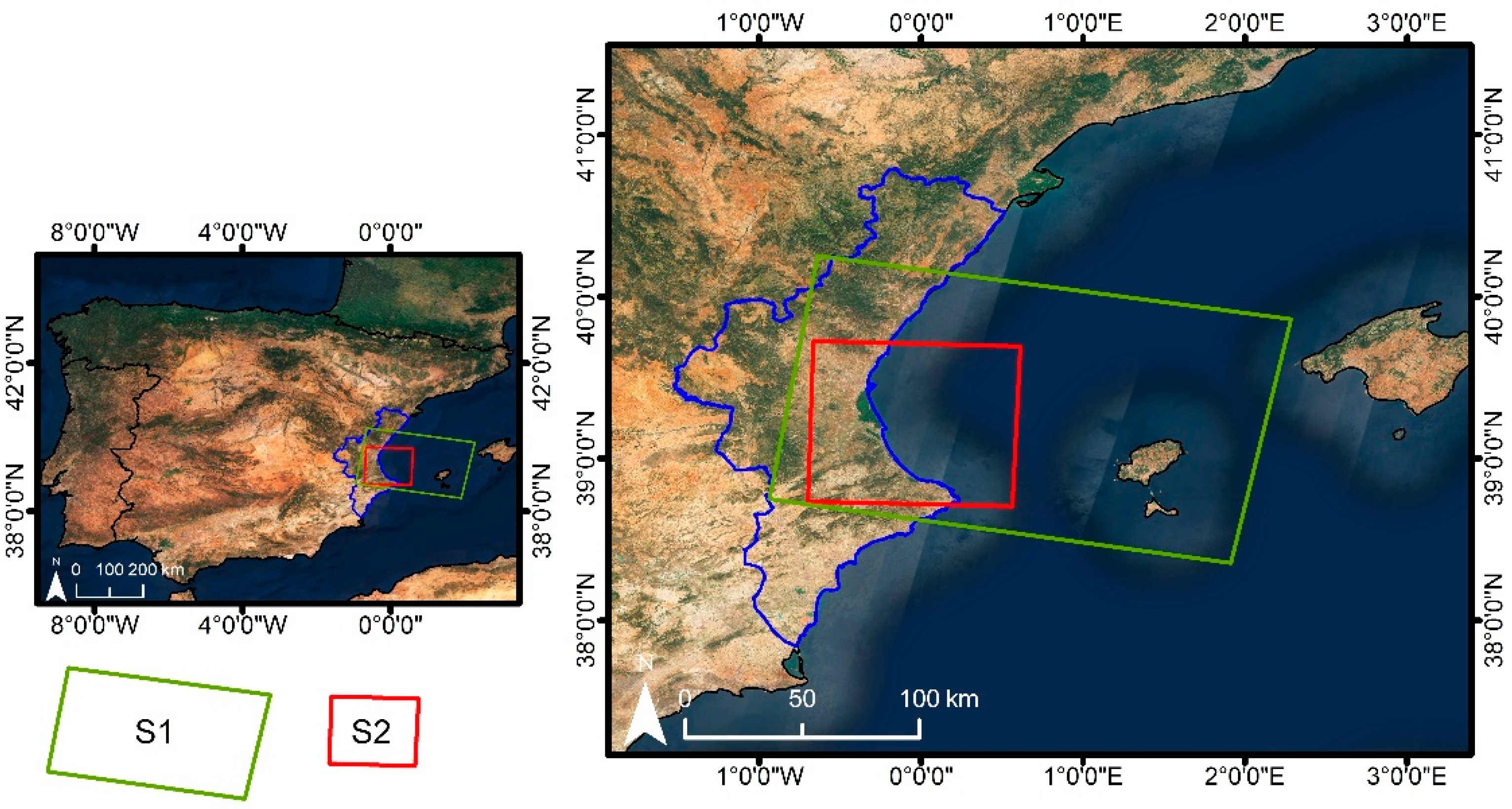
2.1. Study Area
2.2. Sentinel-1 and Sentinel-2 Data
2.3. Sistema de Información Geográfica de Parcelas Agrícolas (SIGPAC)
2.4. Ground Truth
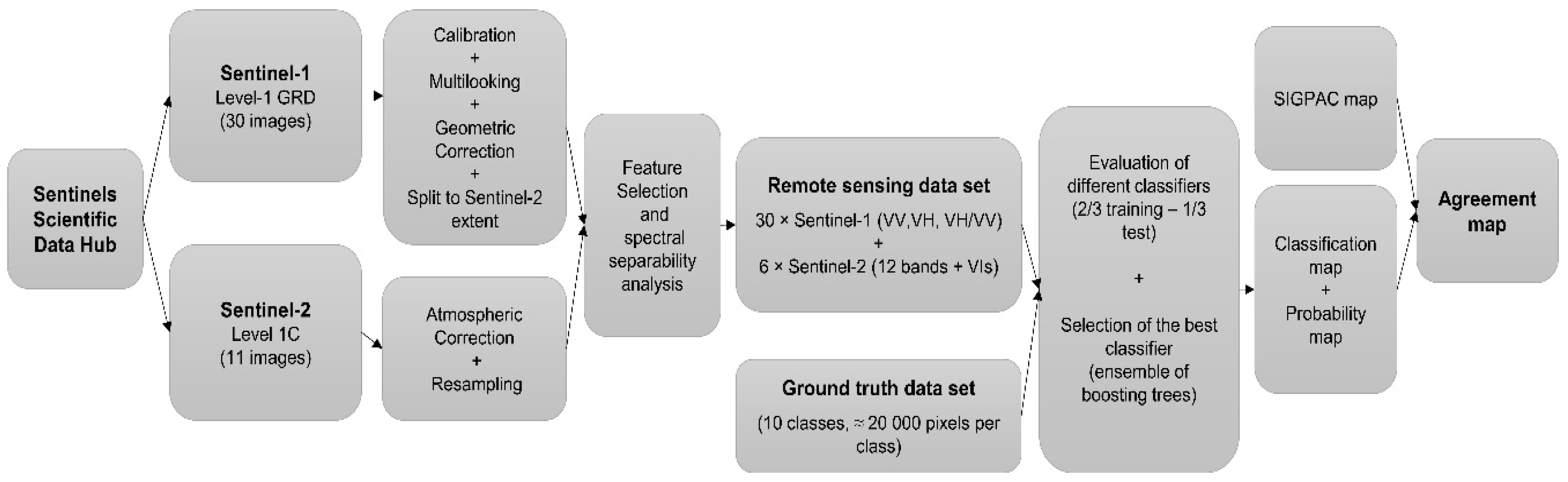
3. Methodology
3.1. Feature Selection
3.2. Classifiers
3.3. Agreement Map
4. Results and Analysis
4.1. Sentinel-2 Spectral Separability Analysis
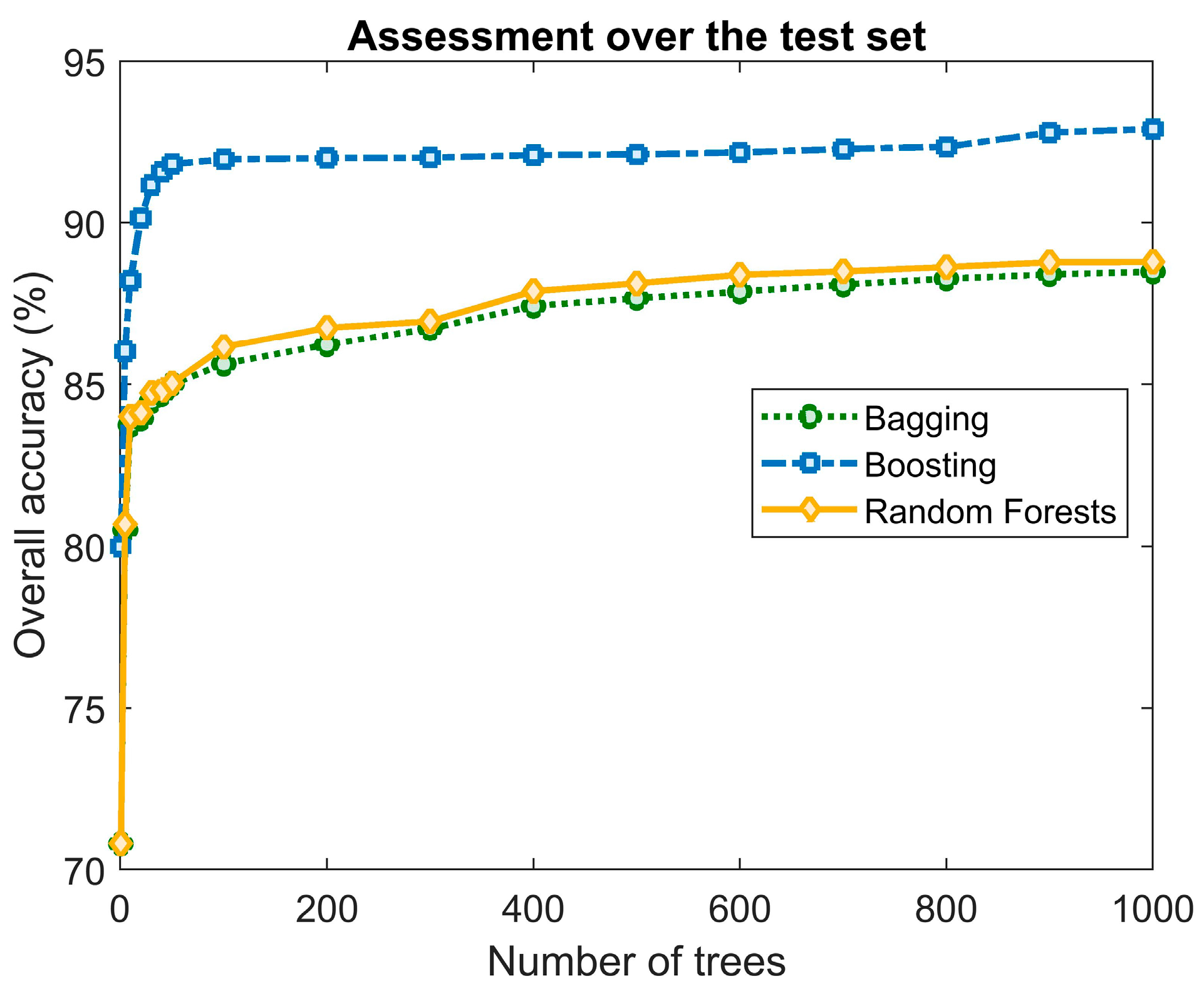
4.2. Accuracy Assessment
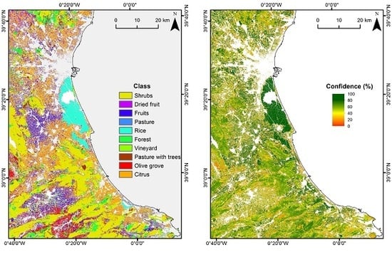
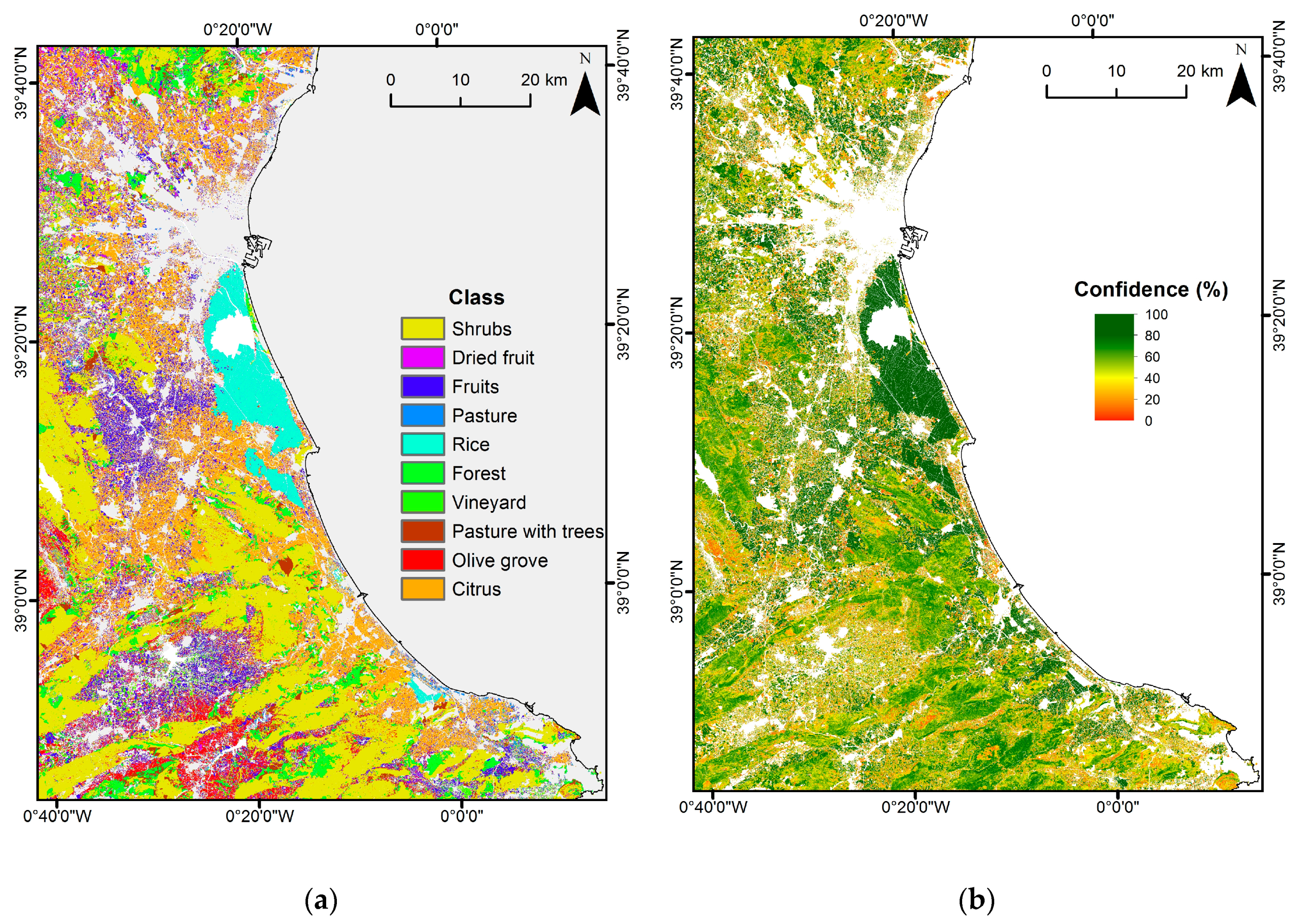
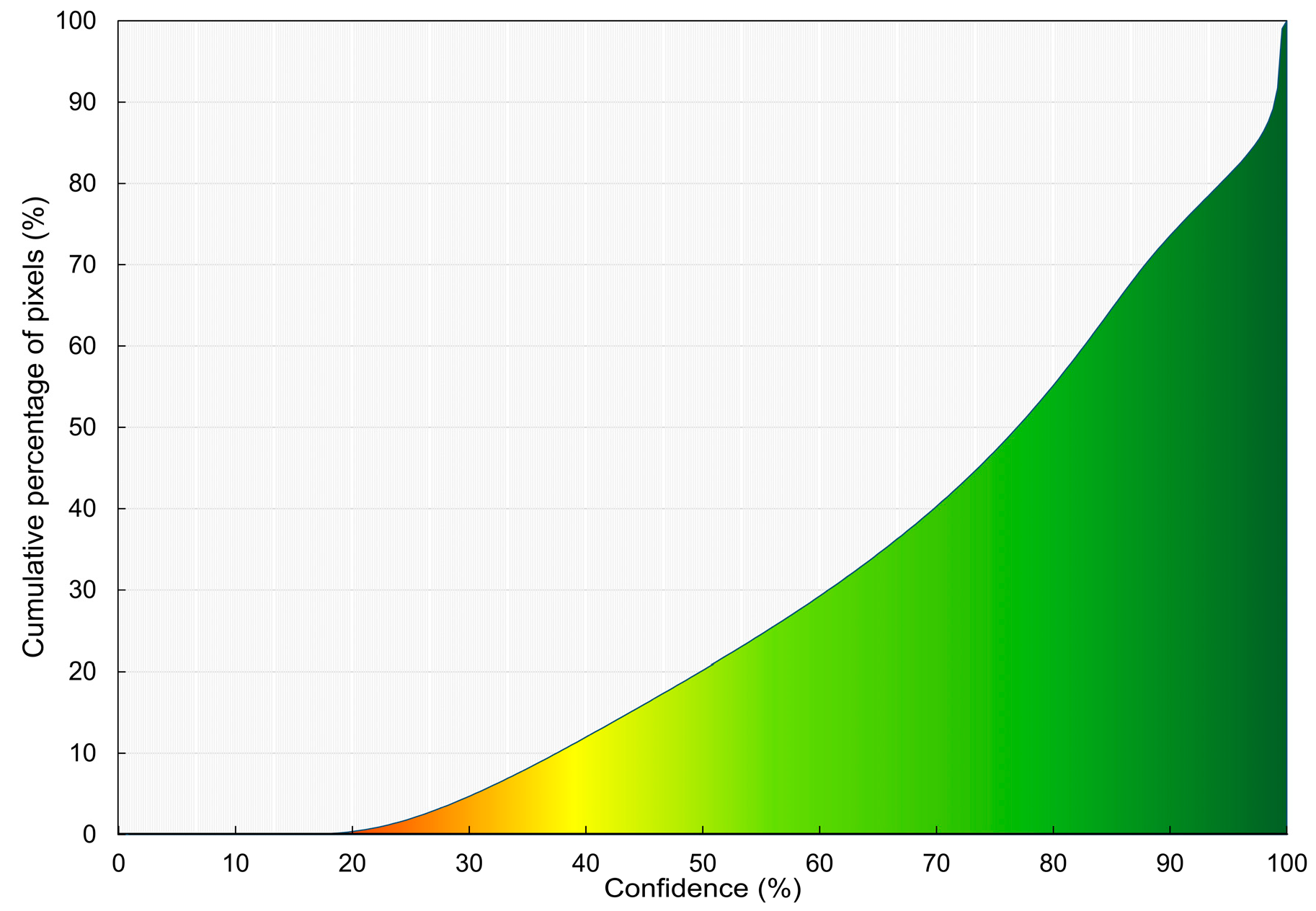
4.3. Classification, Class Probability and Agreement Maps
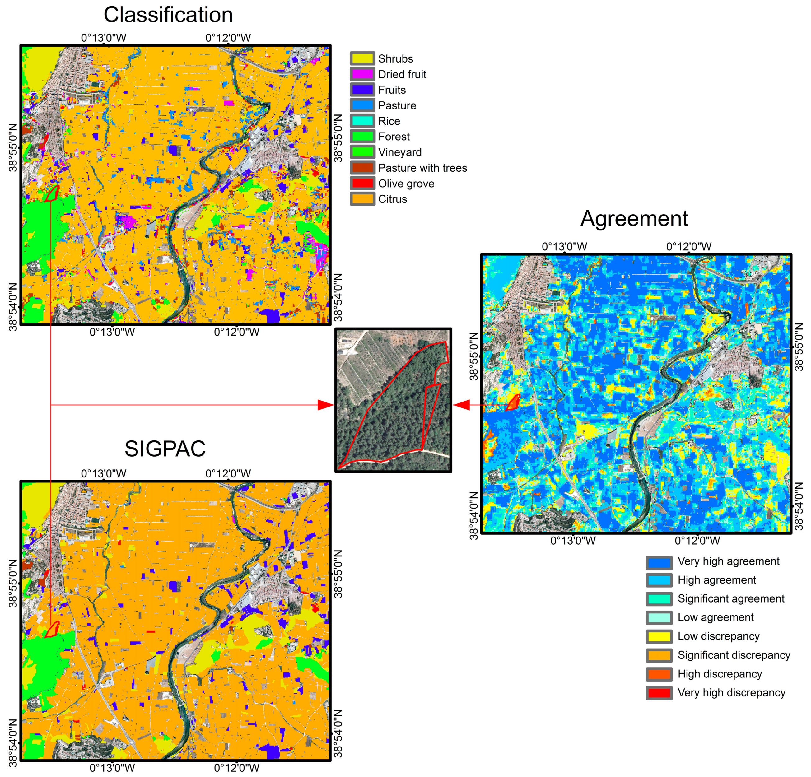
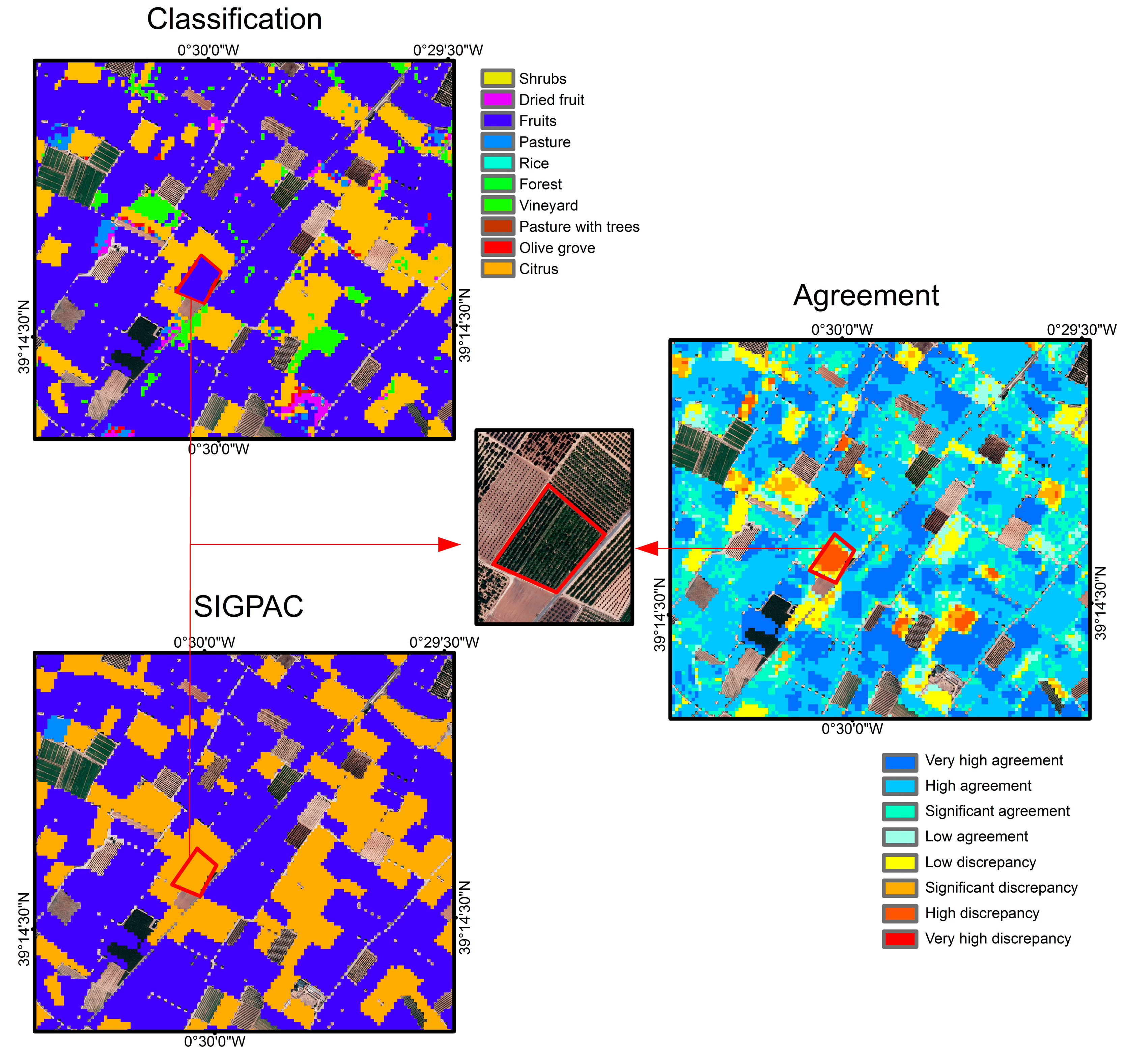
4.4. Utility of the Derived Agreement Map
5. Discussion
6. Conclusions
Supplementary Materials
Author Contributions
Funding
Acknowledgments
Conflicts of Interest
References
- European Commission. Fact Sheet. EU Budget: The Common Agricultural Policy beyond 2020. Available online: http://europa.eu/rapid/press-release_MEMO-18-3974_en.htm (accessed on 1 April 2019).
- European Union. Regulation (EU) No. 1306/2013. Available online: http://eur-lex.europa.eu/LexUriServ/LexUriServ.do?uri=OJ:L:2013:347:0549:0607:EN:PDF (accessed on 1 December 2018).
- European Union. Commission Implementing Regulation (EU) 2018/746 of 18 May 2018 amending Implementing Regulation (EU) No 809/2014 as regards modification of single applications and payment claims and checks. Off. J. Eur. Union 2018, 61, L125CL1. [Google Scholar]
- Friedl, M.A.; Sulla-Menashe, D.; Tan, B.; Schneider, A.; Ramankutty, N.; Sibley, A.; Huang, X. MODIS Collection 5 global land cover: Algorithm refinements and characterization of new datasets. Remote Sens. Environ. 2010, 114, 168–182. [Google Scholar] [CrossRef]
- Congalton, R.G.; Oderwald, R.G.; Mead, R.A. Assessing Landsat Classification Accuracy Using Discrete Multivariate Analysis Statistical Techniques. Photogramm. Eng. Remote Sens. 1983, 49, 1671–1678. [Google Scholar]
- Song, C.; Woodcock, C.E.; Seto, K.C.; Lenney, M.P.; Macomber, S.A. Classification and change detection using landsat tm data: When and how to correct atmospheric effects? Remote Sens. Environ. 2001, 75, 230–244. [Google Scholar] [CrossRef]
- Torres, R.; Snoeij, P.; Geudtner, D.; Bibby, D.; Davidson, M.; Attema, E.; Potin, P.; Rommen, B.; Floury, N.; Brown, M.; et al. GMES Sentinel-1 mission. Remote Sens. Environ. 2012, 120, 9–24. [Google Scholar] [CrossRef]
- Drusch, M.; Del Bello, U.; Carlier, S.; Colin, O.; Fernandez, V.; Gascon, F.; Hoersch, B.; Isola, C.; Laberinti, P.; Martimort, P.; et al. Sentinel-2: ESA’s Optical High-Resolution Mission for GMES Operational Services. Remote Sens. Environ. 2012, 120, 25–36. [Google Scholar] [CrossRef]
- Immitzer, M.; Vuolo, F.; Atzberger, C. First Experience with Sentinel-2 Data for Crop and Tree Species Classifications in Central Europe. Remote Sens. 2016, 8, 166. [Google Scholar] [CrossRef]
- Veloso, A.; Mermoz, S.; Bouvet, A.; Le Toan, T.; Planells, M.; Dejoux, J.-F.; Ceschia, E. Understanding the temporal behavior of crops using Sentinel-1 and Sentinel-2-like data for agricultural applications. Remote Sens. Environ. 2017, 199, 415–426. [Google Scholar] [CrossRef]
- Rüetschi, M.; Schaepman, M.E.; Small, D. Using Multitemporal Sentinel-1 C-band Backscatter to Monitor Phenology and Classify Deciduous and Coniferous Forests in Northern Switzerland. Remote Sens. 2018, 10, 55. [Google Scholar] [CrossRef]
- Belgiu, M.; Csillik, O. Sentinel-2 cropland mapping using pixel-based and object-based time-weighted dynamic time warping analysis. Remote Sens. Environ. 2018, 204, 509–523. [Google Scholar] [CrossRef]
- Van Tricht, K.; Gobin, A.; Gilliams, S.; Piccard, I. Synergistic Use of Radar Sentinel-1 and Optical Sentinel-2 Imagery for Crop Mapping: A Case Study for Belgium. Remote Sens. 2018, 10, 1642. [Google Scholar] [CrossRef]
- Breiman, L.; Friedman, J.; Olshen, R.A.; Stone, C.J. Classification and Regression Trees; Taylor & Francis: London, UK, 1984. [Google Scholar]
- Cover, T.; Hart, P. Nearest neighbor pattern classification. IEEE Trans. Inf. Theory 1967, 13, 21–27. [Google Scholar] [CrossRef]
- Mountrakis, G.; Im, J.; Ogole, C. Support vector machines in remote sensing: A review. ISPRS J. Photogramm. Remote Sens. 2011, 66, 247–259. [Google Scholar] [CrossRef]
- Breiman, L. Random forests. Mach. Learn. 2001, 45, 5–32. [Google Scholar] [CrossRef]
- Pal, M.; Mather, P.M. An assessment of the effectiveness of decision tree methods for land cover classification. Remote Sens. Environ. 2003, 86, 554–565. [Google Scholar] [CrossRef]
- Foody, G.M.; Mathur, A. Toward intelligent training of supervised image classifications: Directing training data acquisition for SVM classification. Remote Sens. Environ. 2004, 93, 107–117. [Google Scholar] [CrossRef]
- Melgani, F.; Bruzzone, L. Classification of hyperspectral remote sensing images with support vector machines. IEEE Trans. Geosci. Remote Sens. 2004, 42, 1778–1790. [Google Scholar] [CrossRef] [Green Version]
- Schneider, A. Monitoring land cover change in urban and peri-urban areas using dense time stacks of Landsat satellite data and a data mining approach. Remote Sens. Environ. 2012, 124, 689–704. [Google Scholar] [CrossRef]
- Vuolo, F.; Neuwirth, M.; Immitzer, M.; Atzberger, C.; Ng, W.-T. How much does multi-temporal Sentinel-2 data improve crop type classification? Int. J. Appl. Earth Obs. Geoinf. 2018, 72, 122–130. [Google Scholar] [CrossRef]
- Blaes, X.; Vanhalle, L.; Dautrebande, G.; Defourny, P. Operational control with remote sensing of area-based subsidies in the framework of the common agricultural policy: What role for the SAR sensors? In Proceedings of the Retrieval of Bio-and Geo-Physical Parameters from SAR Data for Land Applications, Sheffield, UK, 11–14 January 2002; pp. 87–92. [Google Scholar]
- Schmedtmann, J.; Campagnolo, M.L. Reliable Crop Identification with Satellite Imagery in the Context of Common Agriculture Policy Subsidy Control. Remote Sens. 2015, 7, 9325–9346. [Google Scholar] [CrossRef] [Green Version]
- Sitokonstantinou, V.; Papoutsis, I.; Kontoes, C.; Lafarga Arnal, A.; Armesto Andrés, A.P.; Garraza Zurbano, J.A. Scalable Parcel-Based Crop Identification Scheme Using Sentinel-2 Data Time-Series for the Monitoring of the Common Agricultural Policy. Remote Sens. 2018, 10, 911. [Google Scholar] [CrossRef]
- Estrada, J.; Sánchez, H.; Hernanz, L.; Checa, M.J.; Roman, D. Enabling the Use of Sentinel-2 and LiDAR Data for Common Agriculture Policy Funds Assignment. ISPRS Int. J. Geo-Inf. 2017, 6, 255. [Google Scholar] [CrossRef]
- European Court of Auditors. The Land Parcel Identification System: A Useful Tool to Determine the Eligibility of Agricultural Land–but Its Management Could be Further Improved; Publications Office of the European Union: Luxemburg, 2016; ISBN 978-92-872-5967-7. Available online: https://www.eca.europa.eu/Lists/News/NEWS1610_25/SR_LPIS_EN.pdf (accessed on 1 Apr 2019).
- Müller-Wilm, U. Sentinel-2 MSI—Level-2A Prototype Processor Installation and User Manual. Available online: http://step.esa.int/thirdparties/sen2cor/2.2.1/S2PAD-VEGA-SUM-0001-2.2.pdf (accessed on 1 April 2019).
- Hughes, G.P. On the Mean Accuracy of Statistical Pattern Recognizers. IEEE Trans. Inf. Theory 1968, 14, 55–63. [Google Scholar] [CrossRef]
- Richards, J.A. Remote Sensing Digital Image Analysis: An Introduction; Springer: Berlin/Heidelberg, Germany, 2006; pp. 47–54. [Google Scholar]
- Bhattacharyya, A. On a measure of divergence between two statistical populations defined by their probability distributions. Bull. Calcutta Math. Soc. 1943, 35, 99–109. [Google Scholar]
- Rouse, J.W.; Haas, R.H.; Schell, J.A.; Deering, D.W. Monitoring vegetation system in the great plains with ERTS. In Proceedings of the Third Earth Resources Technology Satellite-1 Symposium, Greenbelt, MD, USA, 10–14 December 1973; pp. 3010–3017. [Google Scholar]
- Delegido, J.; Verrelst, J.; Alonso, L.; Moreno, J. Evaluation of Sentinel-2 red-edge bands for empirical estimation of green lai and chlorophyll content. Sensors 2011, 11, 7063–7081. [Google Scholar] [CrossRef] [PubMed]
- Daughtry, C.S.T.; Walthall, C.L.; Kim, M.S.; Brown de Colstoun, E.; McMurtrey, J.E., III. Estimating corn leaf chlorophyll concentration from leaf and canopy reflectance. Remote Sens. Environ. 2000, 74, 229–239. [Google Scholar] [CrossRef]
- Merzlyak, M.N.; Gitelson, A.A.; Chivkunova, O.B.; Rakitin, V.Y. Non-destructive optical detection of leaf senescence and fruit ripening. Physiol. Plant. 1999, 106, 135–141. [Google Scholar] [CrossRef]
- Rondeaux, G.; Steven, M.; Baret, F. Optimization of soil-adjusted vegetation indices. Remote Sens. Environ. 1996, 55, 95–107. [Google Scholar] [CrossRef]
- Vreugdenhil, M.; Wagner, W.; Bauer-Marschallinger, B.; Pfeil, I.; Teubner, I.; Rüdiger, C.; Strauss, P. Sensitivity of Sentinel-1 Backscatter to Vegetation Dynamics: An Austrian Case Study. Remote Sens. 2018, 10, 1396. [Google Scholar] [CrossRef]
- Fukunaga, K. Introduction to Statistical Pattern Recognition; Elsevier: Amsterdam, The Netherlands, 2013. [Google Scholar]
- Prasad, A.M.; Iverson, L.R.; Liaw, A. Newer classification and regression tree techniques: Bagging and random forests for ecological prediction. Ecosystems 2006, 9, 181–199. [Google Scholar] [CrossRef]
- Lodha, S.K.; Fitzpatrick, D.M.; Helmbold, D.P. Aerial lidar data classification using adaboost. In Proceedings of the Sixth International Conference on 3-D Digital Imaging and Modeling, Montreal, QC, Canada, 21–23 August 2007; pp. 435–442. [Google Scholar]
- Cohen, J. A coefficient of agreement for nominal scales. Educ. Psychol. Meas. 1960, 20, 36–47. [Google Scholar] [CrossRef]
- Belgiu, M.; Drăguţ, L. Random Forest in remote sensing: A review of applications and future directions. ISPRS J. Photogramm. Remote Sens. 2016, 114, 24–31. [Google Scholar] [CrossRef]
- Du, P.; Samat, A.; Waske, B.; Liu, S.; Li, Z. Random forest and rotation forest for fully polarized SAR image classification using polarimetric and spatial features. ISPRS J. Photogramm. Remote Sens. 2015, 105, 38–53. [Google Scholar] [CrossRef]
- Stumpf, A.; Kerle, N. Object-oriented mapping of landslides using Random Forests. Remote Sens. Environ 2011, 115, 2564–2577. [Google Scholar] [CrossRef]
- Yan, L.; Roy, D.P. Conterminous United States crop field size quantification from multi-temporal Landsat data. Remote Sens. Environ. 2016, 172, 67–86. [Google Scholar] [CrossRef] [Green Version]
- Immitzer, M.; Toscani, P.; Atzberger, C. The Utility of Wavelet-based Texture Measures to Improve Object-based Classification of Aerial Images. South.-East. Eur. J. Earth Obs. Geomat. 2014, 3, 79–84. [Google Scholar]
- Zhong, L.; Hu, L.; Zhou, H. Deep learning based multi-temporal crop classification. Remote Sens. Environ. 2019, 221, 430–443. [Google Scholar] [CrossRef]
- Kanjir, U.; Đurić, N.; Veljanovski, T. Sentinel-2 Based Temporal Detection of Agricultural Land Use Anomalies in Support of Common Agricultural Policy Monitoring. ISPRS Int. J. Geo-Inf. 2018, 7, 405. [Google Scholar] [CrossRef]
- Dong, J.; Xiao, X.; Kou, W.; Qin, Y.; Zhang, G.; Li, L.; Jin, C.; Zhou, Y.; Wang, J.; Biradar, C.; et al. Tracking the dynamics of paddy rice planting area in 1986–2010 through time series Landsat images and phenology-based algorithms. Remote Sens. Environ. 2015, 160, 99–113. [Google Scholar] [CrossRef]
- Campos-Taberner, M.; García-Haro, F.J.; Camps-Valls, G.; Grau-Muedra, G.; Nutini, F.; Crema, A.; Boschetti, M. Multitemporal and multiresolution leaf area index retrieval for operational local rice crop monitoring. Remote Sens. Environ. 2016, 187, 102–118. [Google Scholar] [CrossRef]
- Campos-Taberner, M.; García-Haro, F.J.; Camps-Valls, G.; Grau-Muedra, G.; Nutini, F.; Busetto, L.; Katsantonis, D.; Stavrakoudis, D.; Minakou, C.; Gatti, L.; et al. Exploitation of SAR and Optical Sentinel Data to Detect Rice Crop and Estimate Seasonal Dynamics of Leaf Area Index. Remote Sens. 2017, 9, 248. [Google Scholar] [CrossRef]
- Brown, S.C.; Quegan, S.; Morrison, K.; Bennett, J.C.; Cookmartin, G. High-resolution measurements of scattering in wheat canopies-Implications for crop parameter retrieval. IEEE Trans. Geosci. Remote Sens. 2003, 41, 1602–1610. [Google Scholar] [CrossRef]
- Mattia, F.; Le Toan, T.; Picard, G.; Posa, F.I.; D’Alessio, A.; Notarnicola, C.; Gatti, A.M.; Rinaldi, M.; Satalino, G.; Pasquariello, G. Multitemporal C-band radar measurements on wheat fields. IEEE Trans. Geosci. Remote Sens. 2003, 41, 1551–1560. [Google Scholar] [CrossRef]
- Lopez-Samchez, J.M.; Ballester-Berman, J.D.; Hajnsek, I. First results of rice monitoring practice in Spain by means of time series of TerraSAR-X dual-pol images. IEEE J. Sel. Top. Appl. Earth Obs. Remote Sens 2011, 4, 412–422. [Google Scholar] [CrossRef]
- Canisius, F.; Shang, J.; Liu, J.; Huang, X.; Ma, B.; Jiao, X.; Geng, X.; Kovacs, J.; Walters, D. Tracking crop phenological development using multi-temporal polarimetric Radarsat-2 data. Remote Sens. Environ. 2018, 210, 508–518. [Google Scholar] [CrossRef]


| 2017 | 2018 | |
|---|---|---|
| Sentinel-1 | 12 April, 24 April, 6 May, 18 May, 30 May, 5 June, 17 June, 29 June, 11 July, 23 July, 4 August, 16 August, 28 August, 9 September, 21 September, 3 October, 15 October, 27 October, 8 November, 20 November, 2 December, 14 December, 26 December. | 7 January, 31 January, 19 January, 12 February, 24 February, 20 March, 8 March. |
| Sentinel-2 | 6 May, 26 May, 15 June, 13 September, 13 October, 2 December, 17 December. | 21 January, 26 May 26, 15 February, 7 March, 27 March. |
| Class | Shrubs | Dried Fruit | Fruits | Pasture | Rice | Forest | Vineyard | Pasture with Trees | Olive Groove | Citrus |
|---|---|---|---|---|---|---|---|---|---|---|
| No. Pixels | 20,382 | 20,703 | 19,800 | 20,058 | 20,157 | 20,478 | 20,295 | 18,846 | 19,434 | 20,385 |
| Vegetation Index | Equation |
|---|---|
| NDVI | |
| OSAVI | |
| NDVI705 | |
| OSAVI705 | |
| MCARI | |
| PSRI |
| Classification Map and SIGPAC | Classification Confidence | Level of Agreement | |
|---|---|---|---|
| Same class | AND | >95% | Very high agreement |
| Same class | AND | 70–95% | High agreement |
| Same class | AND | 50–70% | Significant agreement |
| Same class | AND | <50% | Low agreement |
| Different classes | AND | <50% | Low discrepancy |
| Different classes | AND | 50–70% | Significant discrepancy |
| Different classes | AND | 50–70% | High discrepancy |
| Different classes | AND | >95% | Very high discrepancy |
| JM | SH | DFR | FR | PA | RI | FO | VI | PAT | OL | CI | |
|---|---|---|---|---|---|---|---|---|---|---|---|
| BH | |||||||||||
| SH | 1.750 | 1.597 | 1.508 | 1.996 | 0.636 | 1.870 | 0.253 | 1.497 | 1.879 | ||
| DFR | 2.078 | 0.392 | 0.698 | 1.983 | 1.863 | 0.466 | 1.717 | 0.402 | 1.439 | ||
| FR | 1.603 | 0.218 | 0.621 | 1.985 | 1.760 | 0.672 | 1.538 | 0.250 | 1.472 | ||
| PA | 1.403 | 0.429 | 0.371 | 1.986 | 1.653 | 1.202 | 1.410 | 0.505 | 1.123 | ||
| RI | 6.102 | 4.776 | 4.880 | 4.939 | 1.989 | 1.989 | 1.986 | 1.988 | 1.995 | ||
| FO | 0.382 | 2.679 | 2.120 | 1.752 | 5.228 | 1.951 | 0.296 | 1.713 | 1.899 | ||
| VI | 2.731 | 0.265 | 0.409 | 0.919 | 5.249 | 3.714 | 1.872 | 0.792 | 1.692 | ||
| PAT | 0.135 | 1.955 | 1.465 | 1.221 | 4.991 | 0.160 | 2.752 | 1.446 | 1.837 | ||
| OL | 1.381 | 0.225 | 0.133 | 0.291 | 5.135 | 1.942 | 0.504 | 1.283 | 1.382 | ||
| CI | 2.802 | 1.271 | 1.331 | 0.825 | 6.033 | 2.988 | 1.870 | 2.509 | 1.174 | ||
| Multitemporal Features (Optical + SAR) | Overall Accuracy (%) (κ) | ||||||
|---|---|---|---|---|---|---|---|
| LDA | QDA | k-NN | SVM | RF | Bagging Trees | Boosting Trees | |
| 6 × Sentinel-2 (12 bands) + NDVI 30 × Sentinel-1 (3 bands) | 69.82 (0.68) | 80.36 (0.79) | 84.93 (0.83) | 86.80 (0.85) | 88.69 (0.87) | 88.30 (0.87) | 92.66 (0.90) |
| 6 × Sentinel-2 (12 bands) + OSAVI 30 × Sentinel-1 (3 bands) | 70.58 (0.69) | 80.45 (0.79) | 85.68 (0.84) | 86.97 (0.85) | 88.86 (0.87) | 88.48 (0.87) | 93.58 (0.91) |
| 6 × Sentinel-2 (12 bands) + NDVI705 30 × Sentinel-1 (3 bands) | 67.54 (0.66) | 76.41 (0.75) | 83.29 (0.82) | 85.29 (0.84) | 87.64 (0.86) | 87.23 (0.86) | 90.75 (0.89) |
| 6 × Sentinel-2 (12 bands) + OSAVI705 30 × Sentinel-1 (3 bands) | 70.95 (0.70) | 80.50 (0.79) | 85.94 (0.85) | 86.99 (0.84) | 89.05 (0.88) | 88.76 (0.87) | 93.96 (0.91) |
| 6 × Sentinel-2 (12 bands) + MCARI 30 × Sentinel-1 (3 bands) | 68.93 (0.68) | 77.83 (0.76) | 83.15 (0.82) | 85.04 (0.84) | 88.15 (0.87) | 87.51 (0.86) | 90.15 (0.89) |
| 6 × Sentinel-2 (12 bands) + PSRI 30 × Sentinel-1 (3 bands) | 66.94 (0.66) | 71.60 (0.69) | 76.83 (0.75) | 84.07 (0.83) | 87.10 (0.86) | 87.08 (0.86) | 88.96 (0.88) |
| 6 × Sentinel-2 (12 bands) 30 × Sentinel-1 (3 bands) | 66.73 (0.65) | 70.23 (0.69) | 75.84 (0.74) | 85.59 (0.84) | 86.80 (0.85) | 86.25 (0.85) | 88.19 (0.87) |
| Ground Truth | Total | UA (%) | |||||||||||
|---|---|---|---|---|---|---|---|---|---|---|---|---|---|
| SH | DFR | FR | PA | RI | FO | VI | PAT | OL | CI | ||||
| Classified | SH | 5560 | 19 | 19 | 1 | 0 | 259 | 1 | 329 | 69 | 7 | 6264 | 88.8 |
| DFR | 24 | 6619 | 10 | 1 | 0 | 7 | 5 | 12 | 72 | 12 | 6762 | 97.9 | |
| FR | 70 | 63 | 6450 | 4 | 1 | 36 | 20 | 36 | 87 | 16 | 6783 | 95.1 | |
| PA | 3 | 8 | 1 | 6661 | 0 | 3 | 2 | 1 | 10 | 3 | 6692 | 99.5 | |
| RI | 1 | 1 | 0 | 2 | 6717 | 1 | 0 | 1 | 1 | 0 | 6724 | 99.9 | |
| FO | 455 | 11 | 15 | 5 | 0 | 5845 | 1 | 349 | 38 | 12 | 6731 | 86.8 | |
| VI | 3 | 11 | 18 | 1 | 0 | 0 | 6719 | 1 | 35 | 3 | 6791 | 98.9 | |
| PAT | 500 | 36 | 27 | 2 | 1 | 569 | 0 | 5443 | 50 | 10 | 6638 | 82.0 | |
| OL | 175 | 118 | 53 | 7 | 0 | 105 | 14 | 104 | 6101 | 36 | 6713 | 90.9 | |
| CI | 3 | 15 | 7 | 2 | 0 | 1 | 3 | 6 | 15 | 6696 | 6748 | 99.2 | |
| Total PA (%) | 6794 | 6901 | 6600 | 6686 | 6719 | 6826 | 6765 | 6282 | 6478 | 6795 | OA = 93.96% κ = 0.91 | ||
| 81.8 | 95.9 | 97.7 | 99.6 | 99.9 | 85.6 | 99.3 | 86.6 | 94.2 | 98.5 | ||||
| Multitemporal Features (Optical + SAR) | Overall Accuracy (%) (κ) | ||||||
|---|---|---|---|---|---|---|---|
| LDA | QDA | k-NN | SVM | RF | Bagging Trees | Boosting Trees | |
| 6 × Sentinel-2 (12 bands) + NDVI 30 × Sentinel-1 (3 bands) | 69.82 (0.68) | 80.36 (0.79) | 84.93 (0.83) | 86.80 (0.85) | 88.69 (0.87) | 88.30 (0.87) | 92.66 (0.90) |
| 6 × Sentinel-2 (12 bands) + OSAVI 30 × Sentinel-1 (3 bands) | 70.58 (0.69) | 80.45 (0.79) | 85.68 (0.84) | 86.97 (0.85) | 88.86 (0.87) | 88.48 (0.87) | 93.58 (0.91) |
| 6 × Sentinel-2 (12 bands) + NDVI705 30 × Sentinel-1 (3 bands) | 67.54 (0.66) | 76.41 (0.75) | 83.29 (0.82) | 85.29 (0.84) | 87.64 (0.86) | 87.23 (0.86) | 90.75 (0.89) |
| 6 × Sentinel-2 (12 bands) + OSAVI705 30 × Sentinel-1 (3 bands) | 70.95 (0.70) | 80.50 (0.79) | 85.94 (0.85) | 86.99 (0.84) | 89.05 (0.88) | 88.76 (0.87) | 93.96 (0.91) |
| 6 × Sentinel-2 (12 bands) + MCARI 30 × Sentinel-1 (3 bands) | 68.93 (0.68) | 77.83 (0.76) | 83.15 (0.82) | 85.04 (0.84) | 88.15 (0.87) | 87.51 (0.86) | 90.15 (0.89) |
| 6 × Sentinel-2 (12 bands) + PSRI 30 × Sentinel-1 (3 bands) | 66.94 (0.66) | 71.60 (0.69) | 76.83 (0.75) | 84.07 (0.83) | 87.10 (0.86) | 87.08 (0.86) | 88.96 (0.88) |
| 6 × Sentinel-2 (12 bands) 30 × Sentinel-1 (3 bands) | 66.73 (0.65) | 70.23 (0.69) | 75.84 (0.74) | 85.59 (0.84) | 86.80 (0.85) | 86.25 (0.85) | 88.19 (0.87) |
| Ground Truth | Total | UA(%) | |||||||||||
|---|---|---|---|---|---|---|---|---|---|---|---|---|---|
| SH | DFR | FR | PA | RI | FO | VI | PAT | OL | CI | ||||
| Classified | SH | 5050 | 20 | 32 | 2 | 0 | 409 | 2 | 475 | 67 | 9 | 6066 | 83.3 |
| DFR | 16 | 6519 | 9 | 16 | 0 | 27 | 19 | 16 | 72 | 30 | 6724 | 97.0 | |
| FR | 101 | 111 | 6349 | 17 | 3 | 40 | 70 | 25 | 87 | 40 | 6843 | 92.8 | |
| PA | 3 | 8 | 1 | 6566 | 0 | 21 | 2 | 4 | 37 | 4 | 6646 | 98.8 | |
| RI | 2 | 3 | 0 | 3 | 6714 | 2 | 0 | 3 | 2 | 0 | 6729 | 99.8 | |
| FO | 955 | 11 | 17 | 31 | 0 | 5515 | 1 | 474 | 39 | 14 | 7057 | 78.1 | |
| VI | 13 | 20 | 55 | 2 | 0 | 0 | 6593 | 8 | 97 | 4 | 6792 | 97.1 | |
| PAT | 519 | 34 | 51 | 14 | 2 | 689 | 1 | 5160 | 99 | 11 | 6580 | 78.4 | |
| OL | 129 | 155 | 78 | 32 | 0 | 109 | 62 | 103 | 5962 | 160 | 6790 | 87.8 | |
| CI | 6 | 20 | 8 | 3 | 0 | 14 | 15 | 14 | 16 | 6523 | 6619 | 98.5 | |
| Total PA (%) | 6794 | 6901 | 6600 | 6686 | 6719 | 6826 | 6765 | 6282 | 6478 | 6795 | OA = 91.18% κ = 0.88 | ||
| 74.3 | 94.5 | 96.2 | 98.2 | 99.9 | 80.8 | 97.5 | 82.1 | 92.0 | 96.0 | ||||
© 2019 by the authors. Licensee MDPI, Basel, Switzerland. This article is an open access article distributed under the terms and conditions of the Creative Commons Attribution (CC BY) license (http://creativecommons.org/licenses/by/4.0/).
Share and Cite
Campos-Taberner, M.; García-Haro, F.J.; Martínez, B.; Sánchez-Ruíz, S.; Gilabert, M.A. A Copernicus Sentinel-1 and Sentinel-2 Classification Framework for the 2020+ European Common Agricultural Policy: A Case Study in València (Spain). Agronomy 2019, 9, 556. https://doi.org/10.3390/agronomy9090556
Campos-Taberner M, García-Haro FJ, Martínez B, Sánchez-Ruíz S, Gilabert MA. A Copernicus Sentinel-1 and Sentinel-2 Classification Framework for the 2020+ European Common Agricultural Policy: A Case Study in València (Spain). Agronomy. 2019; 9(9):556. https://doi.org/10.3390/agronomy9090556
Chicago/Turabian StyleCampos-Taberner, Manuel, Francisco Javier García-Haro, Beatriz Martínez, Sergio Sánchez-Ruíz, and María Amparo Gilabert. 2019. "A Copernicus Sentinel-1 and Sentinel-2 Classification Framework for the 2020+ European Common Agricultural Policy: A Case Study in València (Spain)" Agronomy 9, no. 9: 556. https://doi.org/10.3390/agronomy9090556