Retrieval of Evapotranspiration from Sentinel-2: Comparison of Vegetation Indices, Semi-Empirical Models and SNAP Biophysical Processor Approach

Abstract

Remote sensing evapotranspiration estimation over agricultural areas is increasingly used for irrigation management during the crop growing cycle. Different methodologies based on remote sensing have emerged for the leaf area index (LAI) and the canopy chlorophyll content (CCC) estimation, essential biophysical parameters for crop evapotranspiration monitoring. Using Sentinel-2 (S2) spectral information, this study performed a comparative analysis of empirical (vegetation indices), semi-empirical (CLAIR model with fixed and calibrated extinction coefficient) and artificial neural network S2 products derived from the Sentinel Application Platform Software (SNAP) biophysical processor (ANN S2 products) approaches for the estimation of LAI and CCC. Four independent in situ collected datasets of LAI and CCC, obtained with standard instruments (LAI-2000, SPAD) and a smartphone application (PocketLAI), were used. The ANN S2 products present good statistics for LAI (R² > 0.70, root mean square error (RMSE) < 0.86) and CCC (R² > 0.75, RMSE < 0.68 g/m²) retrievals. The normalized Sentinel-2 LAI index (SeLI) is the index that presents good statistics in each dataset (R² > 0.71, RMSE < 0.78) and for the CCC, the ratio red-edge chlorophyll index (CI_red-edge) (R² > 0.67, RMSE < 0.62 g/m²). Both indices use bands located in the red-edge zone, highlighting the importance of this region. The LAI CLAIR model with a fixed extinction coefficient value produces a R² > 0.63 and a RMSE < 1.47 and calibrating this coefficient for each study area only improves the statistics in two areas (RMSE ≈ 0.70). Finally, this study analyzed the influence of the LAI parameter estimated with the different methodologies in the calculation of crop potential evapotranspiration (ET_c) with the adapted Penman–Monteith (FAO-56 PM), using a multi-temporal dataset. The results were compared with ET_c estimated as the product of the reference evapotranspiration (ET_o) and on the crop coefficient (K_c) derived from FAO table values. In the absence of independent reference ET data, the estimated ET_c with the LAI in situ values were considered as the proxy of the ground-truth. ET_c estimated with the ANN S2 LAI product is the closest to the ET_c values calculated with the LAI in situ (R² > 0.90, RMSE < 0.41 mm/d). Our findings indicate the good validation of ANN S2 LAI and CCC products and their further suitability for the implementation in evapotranspiration retrieval of agricultural areas.

1. Introduction

Monitoring the growth of agricultural crops during the whole growing season is important for increasing crop yields and reducing costs and input resources for the agricultural sector [1]. Spatially-explicit knowledge of biophysical variables, such as the leaf area index (LAI) and the chlorophyll content (Chl), is fundamental for the understanding of agricultural ecosystems [2]. Moreover, the variables as LAI are used as inputs of important agricultural models, such as the adapted FAO-56 Penman-Monteith (FAO-56 PM) model [3] which derives the reference (ET_o) and potential (ET_c) crop evapotranspiration. Different empirical methods to estimate evapotranspiration (ET) have been developed over the last 50 years by numerous specialists worldwide. Testing the accuracy of these methods in situ is however time-consuming and costly, and yet ET data are frequently needed at short notice for irrigation scheduling design. The Penman-Monteith model (FAO-56 PM) [3], also referred as the one-step or direct approach, is considered to offer the best results with a minimum possible error. During recent years, there has been a consistent effort to estimate vegetation parameters from remotely sensed data, allowing to adapt the Penman-Monteith equation for direct use with Earth observation (EO) based LAI and surface albedo retrieval [4], minimizing time and cost. Consequently, nowadays it is the most commonly used method for the estimation of ET [5,6,7].

LAI is defined as the one half of the total leaf area per unit horizontal ground surface area (m² leaf per m² surface or dimensionless) [8] and Chl is given by the weight of green pigment per leaf surface (g Chl per m² leaf) [9]. By quantifying and monitoring both parameters, the photosynthetic capacity [10,11], nutrient stress [12,13] and development stage [14,15] of crops can be detected. There are two approaches to remotely estimate Chl in crops. One of them is by the assessment of the leaf chlorophyll content (LCC) [16] and the other approach is based on canopy chlorophyll content (CCC), the total crop chlorophyll content, which is defined as the product of LCC and LAI [17]. Different studies have demonstrated that a direct estimation of CCC is more robust and accurate than an estimation based on the product of the individual estimation of LAI and LCC [18]. Therefore, the remote estimation of CCC has been preferred the one of the LCC.

The direct field measurements of biophysical parameters require continuous updates and can be extremely time-consuming and expensive [19]. Therefore, remote sensing from satellite, aerial and unmanned aerial vehicle platforms has become a popular technique for monitoring agricultural areas because of its ability to acquire synoptic information at different times and spatial scales [20,21]. There are different approaches for estimating biophysical parameters from remotely sensed data, i.e., (1) empirical retrieval methods, which consist of relating the biophysical parameter of interest against spectral data (e.g., vegetation indices—VIs), (2) statistical category, which defines regression functions according to information from remote sensing data (e.g., artificial neural network—ANN) and (3) physically-based retrieval methods, which refers typically to the inversion of radiative transfer models (RTMs) against remote sensing observations.

The empirical approaches provide an acceptable level of accuracy in the estimation of important biophysical parameters and can be calculated without high computational demands, but due to the sensitivity of VIs to vegetation type, the site and sensor characteristics, reliable ground measurements are required for model calibration. Furthermore, VIs are affected by the canopy structure, given different leaf angles, leaf spatial distribution and row orientation, which strongly influences canopy reflectance, which is further influenced by soil optical properties and sun-target-sensor geometry [15]. Additionally, VIs are generally based on only a few spectral bands and a single-angle observation, leading to an under-exploitation of the full spectral and directional range available from new generation sensors. Despite the above, there are VIs based models that have been improved because they also account for other factors such as the bare soil response affecting the canopy reflectance, as is the case of the Clevers leaf area index by reflectance (CLAIR) model [22].

The statistical methods can be either parametric or non-parametric [23]. Parametric models rely on physical knowledge of the problem and build explicit parameterized expressions, assuming a finite set of parameters. Therefore, the complexity of the model is bounded even if the amount of data is unbounded. This makes them quite inflexible. Alternatively, non-parametric models are adjusted to predict a variable of interest using a training dataset of input-output data pairs, building a non-linear regression model using the observed parameters as inputs and without taking into account physical restrictions. This makes them more flexible.

On the other hand, the physically based models of canopy reflectance consider the crop architecture, illumination, soil backgrounds and viewing geometries, making them applicable across multiple operational applications for crop biophysical parameters retrieval [24]. Nevertheless, other restrictions, such as the intrinsic risk of oversimplifying the architecture of canopy for those RTMs fast enough for operational applications, have to be considered in this context [25]. They generally correspond to a simple description of canopy architecture which may not represent the actual one, particularly regarding the clumped nature of many vegetation types. Moreover, in these approaches, radiometric measurement uncertainties have to be added to the simulations when building up the training datasets [26]. The ill-posed problem has to be taken also into account when performing model inversion: The different parameter combinations may produce almost identical spectra, resulting in significant uncertainties in parameter estimation [27].

For agricultural monitoring by remote sensing, the spatial resolution should be at least 20 m and, preferably, 10 m in order to make site-specific management possible [28]. A temporal resolution of less than a week would be required to follow-up acute changes in the crop condition and provide a timely response in management practices. Specifically, extensive research has been carried out on ET crop estimation for management strategies using EO data, but to date, one of the major limitations for their applicability and technological transfer was the limited spatial and temporal resolution of the sensors [29]. In this context, the Sentinel-2 (S2) mission from the European Space Agency (ESA) [30] fulfills such operational requirements. S2 is a constellation of satellites, Sentinel-2A (S2A) and Sentinel-2B (S2B) at the moment, launched by the ESA on 23 June, 2015 and 7 March, 2017, respectively. They occupy the same sun-synchronous orbit at an altitude ~786 km, but are separated by 180°. Together, they provide better than 5-day revisit of the Earth’s land surfaces under cloud-free conditions with a 10, 20 and 60 m of pixel size. S2A and S2B carry on board a virtually identical sensor, named the multi-spectral imager (MSI), covering the visible, the near-infrared (NIR) and the shortwave-infrared (SWIR) spectral regions. Hence, the S2 mission improves the temporal, spatial and spectral resolution of remote sensing data, compared to other multi-spectral missions, such as Landsat, and offers great opportunities for agricultural monitoring. For S2, the operational biophysical parameter products associated with a quality indicator are provided through the Sentinel Application Platform (SNAP) toolbox and produced through an ANN which has been trained by simulated spectra generated from well-known RTMs [31]. However, the accuracy of these products has been poorly tested, producing mostly improvable results [32,33]. It should be mentioned that both the S2 satellite images and the SNAP program are free of charge.

The present work aims at evaluating empirical (VIs), semi-empirical (CLAIR model) and ANN S2 products derived from SNAP biophysical processor methods for LAI and CCC estimation, the essential parameters to understand the evapotranspiration process. Section 2.1 describes the four test sites used in this study, a strong point of this research as they are totally independent zones with their specific characteristics. Section 2.2 details the field measurement protocol followed for the measurement of the LAI and LCC parameters in each of the zones, as well as the field instrument calibration equations. Section 2.3 specifies the four datasets obtained from the field campaigns, detailing the crop types sampled and the number of samples of each crop type, among other characteristics. From these in situ data and the corresponding S2 spectral information, the ANN S2 products are applied (Section 2.4), as well as the semi-empirical CLAIR model and the most commonly VIs used by the literature for the estimation of LAI and CCC (Section 2.5). Section 2.6 describes the FAO-56 PM equation adapted to remote sensing, specifying where the LAI parameter is within the equation. Section 3 details the results obtained for the estimation of the LAI and CCC parameters with each of the methodologies, as well as the impact obtained from the LAI parameter on the FAO-56 PM equation. Finally, Section 4 evaluates the results, highlighting the positive and negative aspects of each method and comparing with other studies. Section 5 outlines the main conclusions, specifying the most optimal methodology for LAI and CCC retrieval and for the evapotranspiration estimation from the operational point of view.

2. Materials and Methods

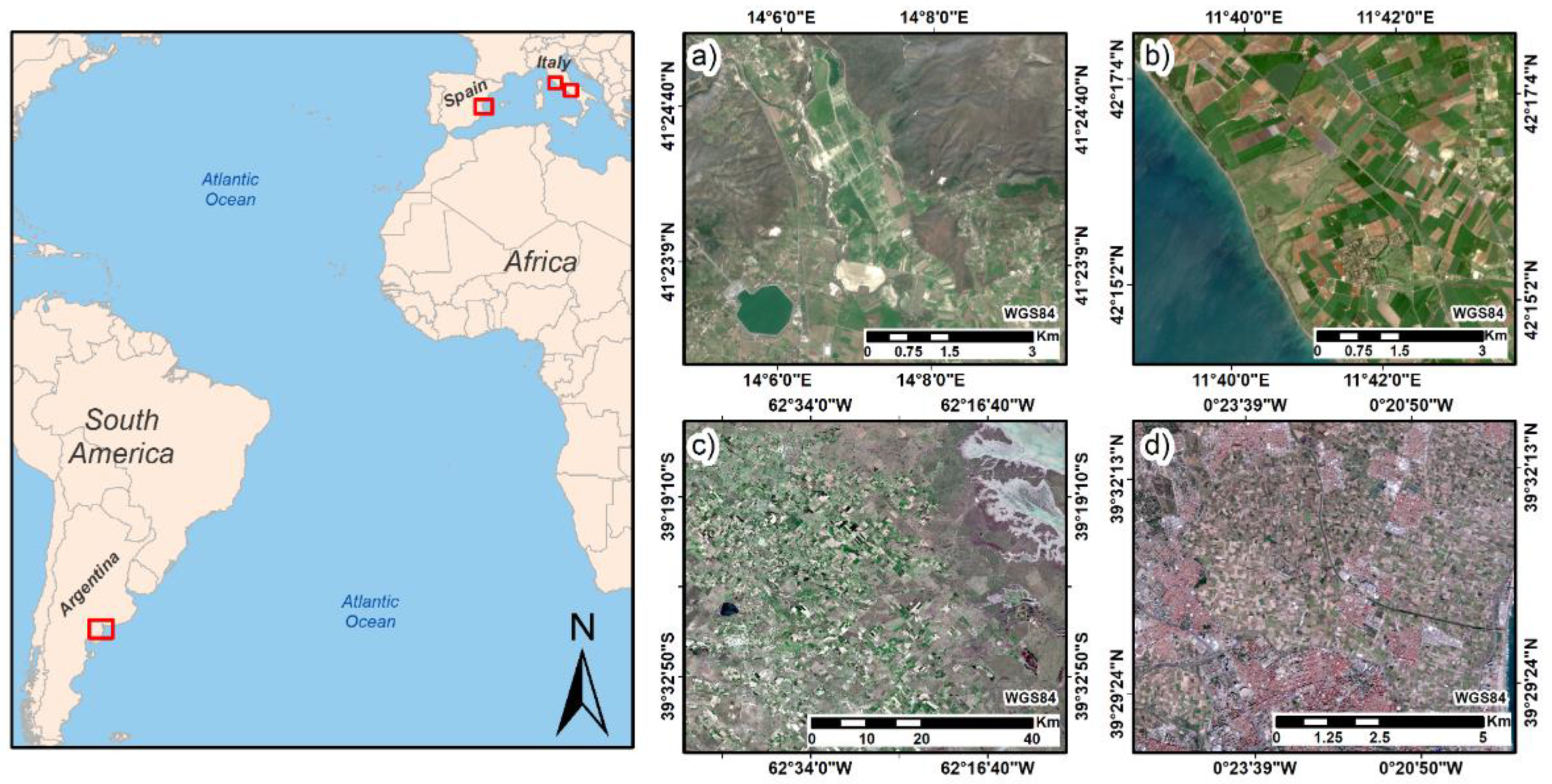
2.1. Study Sites

Four different test areas have been used in this study. Two study sites are located in Italy, another in Argentina and, finally, one in Spain (Figure 1).

2.1.1. Caserta (Italy)

One test site is an Italian agricultural area near Caserta (study site central coordinates 41°24′8.86″N, 14°6′54.24”E, 134 m a.s.l., Datum WGS84), located 30 km from the coast. The climate is Mediterranean, but with a marked continental influence. Due to this influence, abrupt seasonal and daily temperature changes are produced, with an average annual temperature of 15.2 °C, but with hot and dry summers, with temperatures easily exceed 30 °C (July, August) and winters with temperatures close to 5 °C (December, January). The annual rainfall is approximately 580 mm, occurring mainly during autumn and winter [34]. This agricultural area is mainly composed of oat and alfalfa irrigated crop types, cultivated in plots in size of more than 100 m in length.

2.1.2. Tarquinia (Italy)

The second test site located in Italy is an agricultural area near Tarquinia municipality (study site central coordinates 42°17′12.30″N, 11°41′8.83″E, 25 m a.s.l., Datum WGS84), being 3 km from seashore. The climate is typical Mediterranean characterized by warm dry summers, mild winters, and with an average annual rainfall of approximately 600 mm, mainly concentrated in autumn and spring. The mean daily temperature is 15.3 °C (ranging from 7.7 °C in January and of 23.7 °C in July) [35]. The area is characterized by intensive agricultural management due to the production of irrigated crops, mainly tomato, cultivated in plots with a size smaller than 100 m in length.

2.1.3. Bahía Blanca (Argentina)

The third study area is located in the Buenos Aires province, south of Bahía Blanca (study site central coordinates 39°3′53.32″S, 62°40′21.50″W, 26 m a.s.l., Datum WGS84). It is situated in a plain with slopes that descend towards the coast. The climate is temperate, sub-humid with moderate temperatures but with high variability (ranging from 23 °C in January and of 7.6 °C in July) and there is no dry season. The average annual rainfall is 385 mm, being the rainiest months: February, March, October and November [36]. The study area is far from the coast in a range of 40 - 100 km. This test site is composed of irrigated and rain-fed multi-crop types, mainly wheat, onion and oat crop types, cultivated in plots of size larger than 300 m in length.

2.1.4. Valencia (Spain)

The last study site is located around Valencia city (Spain), in an area named Huerta of Valencia (study site central coordinates 39°31′11.73″ N, 0°23′20.48″ W, 18 m a.s.l., Datum WGS84). It is a zone in an alluvial plain with an approximate area of 12,000 hectares, located 6 km from the sea. The climate is typically Mediterranean with mild winters and hot dry summers and a yearly average temperature of approximately 18 °C (ranging from 11.8 °C in January and 25.6 °C in July). The seasonal rainfall is minimal in summer and maximal in autumn and spring, with an average annual value of 230 mm [37]. A complex historical irrigation system based on irrigation ditches brings water to this fertile soil in which cereals, vineyards and olive trees were originally the main crops. Nowadays, they have been replaced by rice, tigernut and new species of vegetables and citric orchards. All these crop types are currently cultivated in plots in size of 40–100 m in length (< 1 ha).

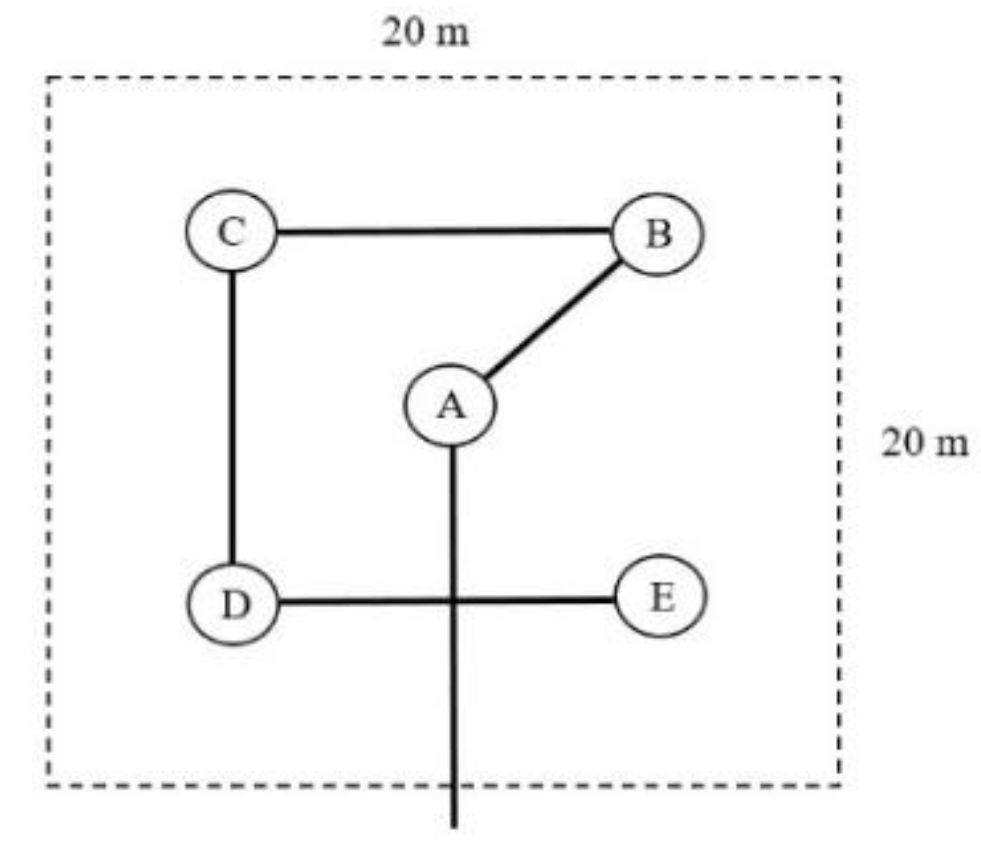
2.2. Field Measurement Protocol

The measurements were collected following the Land European Remote-Sensing Instruments (VALERI) field protocol [38]. The VALERI protocol is a sampling strategy corresponding to high spatial-resolution satellite imagery, choosing elementary sampling units (ESUs) of 20 m × 20 m for each measuring plot. Each ESU was chosen in the middle of the crop field, keeping a minimum distance of 20 m from the edges of the field. To account for the spatial LAI and LCC variability within each ESU, the measuring points were sampled following a square spatial sampling with 5 random measurements at each point (A, B, C, D and E), providing a statistically mean LAI and LCC estimate per ESU (Figure 2). The center of the ESU (sampling point A) was geo-located using a GPS providing an accuracy of less than 5 m for later matching the mean LAI and LCC estimate with the corresponding S2 reflectance data.

In the different field campaigns, the LAI and LCC biophysical parameter data were taken with different instruments. The LAI measurements were carried out by using the Plant Canopy Analyzer instruments LAI-2000 and LAI-2200 (Li-COR Inc., Lincoln, NE, USA) and PocketLAI smartphone application (University of Milan, DiSAA, Cassandra lab, version 1.6.5.2c) [39]. The LCC parameter, on the other hand, was taken with the MC-100 Chlorophyll Concentration Meter (MC) (Apogee Instruments, Inc., Logan, UT, USA) and Chlorophyll Meter SPAD-502Plus (SPAD) (Konica Minolta Optics Inc., Japan). The field sampling protocol was identic for all study sites and instruments. Since the MC and SPAD instruments provide digital count values, a calibration equation is required to finally obtain the chlorophyll content. In the case of the MC instrument, it uses a calibration equation specific to each crop type. In this study, the equations for wheat (Equation (1)) and for tomato crop type (Equation (2)) were used concretely [40]. In the case of the SPAD instrument, an adjusted calibration equation for many plant species was used, so Equation (3) was applied as the standard equation for all crop types [9].

$$\left(\mathrm{wheat}\right)\mathrm{LCC}\left(\frac{\mathrm{g}}{{\mathrm{m}}^2}\right)=\left(-84+79{\mathrm{MC}}^{0.6}\times 0.9\right)/1000$$

(1)

$$\left(\mathrm{tomato}\right)\mathrm{LCC}\left(\frac{\mathrm{g}}{{\mathrm{m}}^2}\right)=\left(-328+304{\mathrm{MC}}^{0.26}\times 0.9\right)/1000$$

(2)

$$\left(\mathrm{standard}\right)\mathrm{LCC}\left(\frac{\mathrm{g}}{{\mathrm{m}}^2}\right)=\left(0.021752{\mathrm{SPAD}}^{2.1129}\right)/100$$

(3)

2.3. Datasets

Table 1. Mean values and standard deviation (SD) of the obtained variables for each crop species and test site.

Test Site	Crop Types	N° ESUs	LAI		LCC (g/m2)		Total ESUs
			Mean	SD	Mean	SD
CAS19_IT	Oat (Avena sativa)	44	2.65	0.93	0.96	0.15	50
	Ryegrass (Secale cereale)	3	2.22	0.14	0.45	0.27
	Alfalfa (Medicago sativa)	3	1.58	0.25	0.96	0.09
	Bare soil	10	0	0	0	0	10
TAR16_IT	Wheat (Triticum durum)	18	3.24	0.98	0.45	0.07	44
	Tomato (Solanum lycopersicum)	26	2.15	1.10	0.37	0.07
	Bare soil	10	0	0	0	0	10
BAH18_AR	Wheat (Triticum durum)	8	1.51	1.28	0.50	0.07	50
	Alfalfa (Medicago sativa)	5	2.11	0.78	0.71	0.18
	Onion (Allium cepa)	9	1.65	0.83	0.36	0.10
	Oat (Avena sativa)	6	2.51	0.63	0.47	0.17
	Agropiro (Thinopyrum ponticum)	9	3.24	0.95	0.57	0.10
	Barley (Hordeum vulgare)	4	2.43	1.23	0.50	0.02
	Potato (Solanum tuberosum)	9	2.09	0.52	0.64	0.06
	Bare soil	12	0	0	0	0	12
VAL18_ES	Tigernut (Cyperus esculentus)	7	1.78	0.64	0.28	0.09	48
	Potato (Solanum tuberosum)	2	0.95	0.15	0.73	0.03
	Orange tree (Citrus x sinensis)	7	2.68	0.41	1.40	0.29
	Pumpkin (Cucurbita maxima)	4	1.54	0.36	0.52	0.23
	Artichoke (Cynara scolymus)	6	1.94	0.35	0.98	1.12
	Alfalfa (Medicago sativa)	3	2.33	0.22	0.82	0.09
	Lettuce (Lactuca sativa)	5	3.15	0.90	0.34	0.08
	Oleander (Nerium oleander)	5	1.64	0.78	1.08	0.30
	Onion (Allium cepa)	2	0.44	0.01	0.39	0.04
	Walnut tree (Juglans regia)	2	1.16	0.18	0.79	0.02
	Olive tree (Olea europaea)	2	2.50	0.67	1.39	0.09
	Fan palm (Chamaerops humilis)	3	2.26	0.44	1.07	0.04
	Bare soil	10	0	0	0	0	10

summarizes the characteristics of the four datasets used in this study. On the one hand, the field data of Caserta (Italy) were taken with LAI-2000 and SPAD, during the days 12 and 20 March, 2019, obtaining a dataset composed of 50 mean LAI and CCC (LAI × LCC) values of three different crop types. This dataset is hereafter called “CAS19_IT”. Regarding Tarquinia dataset, hereafter called “TAR16_IT”, is composed of 44 mean LAI and CCC values of two common crop types, taken with LAI-2000 and MC instruments during several dates to cover a wider variety of growth stages (17 March, 19 April, 6 May, 8 and 25 June, 8 and 28 July, 2016). The other two datasets are composed of multi-crop data. A dataset obtained in Argentina (“BAH18_AR”), composed of 50 LAI and CCC mean values taken with PocketLAI and SPAD during 16, 17, 21 and 23 November 2018. Further, another taken in Huerta of Valencia (Spain), hereafter called “VAL18_ES”, composed of 48 LAI and CCC mean values obtained on 1, 3 and 4 October 2018. Furthermore, bare soil ESUs were included in all datasets (LAI = 0, LCC = 0 g/m²), with the aim of creating a more robust and general method. All datasets are covering a wide range of crop LAI values, i.e., from 0 to 5, and CCC values, i.e., from 0 to 5.4 g/m², providing an optimal basis for the definition of a new general methodology.

2.4. Sentinel-2 Imagery and SNAP Biophysical Processor Products

All field campaigns were carried out on days close to the overpass dates of S2 over the study area with a maximum difference of three days. The technical characteristics of the MSI on-board the S2 satellites are outlined in

Table 2. S2 band setting. The eight bands used for leaf area index (LAI) and canopy chlorophyll content (CCC) automatic estimation are highlighted.

Band Number	Function	Central Wavelength (nm)	Bandwidth (nm)	Spatial Resolution (m)
B1	Coastal aerosol	443	27	60
B2	Blue	490	98	10
B3	Green	560	45	10
B4	Red	665	38	10
B5	Vegetation red-edge	705	19	20
B6	Vegetation red-edge	740	18	20
B7	Vegetation red-edge	783	28	20
B8	Near-infrared (NIR)	842	145	10
B8a	Vegetation red-edge	865	33	20
B9	Water vapour	945	26	60
B10	SWIR	1380	75	60
B11	SWIR	1610	143	20
B12	SWIR	2190	242	20

[41]. The images were downloaded directly and free of charge from the ESA server [42]. ESA provides Level-1C (L1C) images, which were geometrically corrected with top-of-atmosphere (TOA) reflectance and, in some places, Level-2A (L2A) images, which were geometrically and atmospherically corrected, with top-of-canopy (TOC) reflectance. Two available cloud-free L1C acquisitions of S2 over Caserta were downloaded, seven over Tarquinia, three over Argentina and one over Spain (

Table 3. Satellite images used in this study with field measurement dates.

Test Site	Sentinel-2 Tile	N° of Images	Acquisition Dates	Field Measurement Dates
CAS19_IT	T33TVF	2	2019 (March 09, March 19)	2019 (March 12, March 20)
TAR16_IT	T32TQM	7	2016 (March 17, April 19, May 06, June 08, June 25, July 08, July 28)	2016 (March 17, April 19, May 06, June 08, June 25, July 08, July 28)
BAH18_AR	T20HNB T20HNC	3	2018 (November 18, November 23)	2018 (November 16, November 17, November 21, November 23)
VAL18_ES	T30SYJ	1	2018 (October 03)	2018 (October 01, October 03, October 04)

). These images were atmospherically corrected using the Sen2Cor processor (version 2.5.5) available in the SNAP toolbox (version 6.0), converting TOA reflectance into TOC reflectance [43]. Further, they were resampled to 10 m pixel size with all selected pixels falling entirely inside the corresponding ESU, obtaining the TOC reflectance spectrum for each ESU.

The SNAP toolbox additionally provides a scientific tool named the Biophysical Processor for the retrieval of LAI, CCC, canopy water content (CWC), fraction of photosynthetically active radiation absorbed (fAPAR) by the canopy green elements and the fraction of vegetation cover (FVC) variables. The retrieval algorithms for these parameters are based on an ANN approach, trained with a globally representative set of simulations from a canopy RTM (PROSAIL: PROSPECT [44] + SAIL [45]). The ANN algorithm hereby requires the input of eight S2 spectral bands (B3–B7, B8a, B11 and B12), which are all resampled to 10 m pixel size to derive LAI and CCC parameters. Additional, the quality indicators are attached to these SNAP biophysical products [31]. Through the Biophysical Processor, the LAI and CCC values together with the quality indicators from each ESU of all datasets were automatically obtained.

2.5. Semi-Empirical and Empirical Methods

To compare the ANN S2 products approach with semi-empirical and empirical ones, the LAI parameter was obtained with the CLAIR model and commonly used LAI VIs and CCC through the most commonly used VIs.

2.5.1. Semi-Empirical Method: The CLAIR Model

The simple and feasible approaches based on empirical relationships between LAI and nadir-viewing measurements in the red and near-infrared bands have been defined by several authors. One of these methods is the semi-empirical CLAIR model [22]. It is based on the logarithmic relationship between LAI and the Weighted Differences Vegetation Index (WDVI), using a soil line value to compensate for the errors related to soil background reflectance [46]:

$$\mathrm{LAI}=-\frac{1}{{\mathsf{\alpha }}^{*}}\ln \left(1-\frac{\mathrm{WDVI}}{{\mathrm{WDVI}}_{\infty }}\right)$$

(4)

$$\mathrm{WDVI}={\mathrm{R}}_{\mathrm{i}}-{\mathrm{R}}_{\mathrm{r}}\frac{{\mathrm{R}}_{\mathrm{soil},\mathrm{i}}}{{\mathrm{R}}_{\mathrm{soil},\mathrm{r}}}$$

(5)

$${\mathrm{WDVI}}_{\infty }={\mathrm{WDVI}}_{\mathrm{mean}}+6{\mathrm{WDVI}}_{\mathrm{SD}}$$

(6)

where α* is an extinction coefficient expressing the increase of WDVI for a unitary increase of LAI, i.e., an empirical shape parameter, mainly depending on canopy architecture and computed from field measurements corresponding to the minimum error between the observed and estimated LAI. In this study, the commonly fixed values of 0.41 for herbaceous crop and 0.30 for tree were used [47,48]. The R_i and R_r variables indicate the reflectance of the observed canopy in near-infrared (B8—842 nm) and red (B4—665 nm) bands respectively, while R_soil,i and R_soil,r are the corresponding values for bare soil conditions. The ratio R_soil,i/R_soil,r can be taken as the constant and is called the soil line slope [46]. In this work, the soil line slope was automatically estimated for each image, masking the vegetation, water and cloud pixels first with the Scene Classification (SCL) map derived by Sen2Cor and using the scatter plot between B4 and B8 S2 bands of all bare soil pixels [49]. Finally, ${\mathrm{WDVI}}_{\infty }$ is the asymptotical value of WDVI for LAI→∞, and is calculated at each acquisition at the target “vegetation cover (not woody) very dense and uniform” or maximum vegetation (agricultural) cover. In order to estimate this number automatically, the WDVI index was applied to the whole S2 image and with the SNAP statistics estimation option, the mean (WDVI_mean) and standard deviation (WDVI_SD) were calculated and used in Equation (6).

2.5.2. Empirical Method: Established Vegetation Indices

Table 4. Established LAI and CCC indices used in this study. R_λ represents reflectance at the wavelength λ (nm). The specific S2 band number to be used in each index is specified.

LAI
Reference	Abbreviation	Formula	Formula with S2 Bands
[50]	RVI	$\frac{{\mathrm{R}}_{842}}{{\mathrm{R}}_{665}}$	$\frac{\mathrm{B}8}{\mathrm{B}4}$
[51]	NDVI	$\frac{{\mathrm{R}}_{842}-{\mathrm{R}}_{665}}{{\mathrm{R}}_{842}+{\mathrm{R}}_{665}}$	$\frac{\mathrm{B}8-\mathrm{B}4}{\mathrm{B}8+\mathrm{B}4}$
[52]	NDI	$\frac{{\mathrm{R}}_{705}-{\mathrm{R}}_{665}}{{\mathrm{R}}_{705}+{\mathrm{R}}_{665}}$	$\frac{\mathrm{B}5-\mathrm{B}4}{\mathrm{B}5+\mathrm{B}4}$
[53]	RENDVI	$\frac{{\mathrm{R}}_{842}-{\mathrm{R}}_{740}}{{\mathrm{R}}_{842}+{\mathrm{R}}_{740}}$	$\frac{\mathrm{B}8-\mathrm{B}6}{\mathrm{B}8+\mathrm{B}6}$
[33]	SeLI	$\frac{{\mathrm{R}}_{865}-{\mathrm{R}}_{705}}{{\mathrm{R}}_{865}+{\mathrm{R}}_{705}}$	$\frac{\mathrm{B}8\mathrm{a}-\mathrm{B}5}{\mathrm{B}8\mathrm{a}+\mathrm{B}5}$
[54]	TRBI	$\frac{{\mathrm{R}}_{560}+{\mathrm{R}}_{665}}{{\mathrm{R}}_{842}}$	$\frac{\mathrm{B}3+\mathrm{B}4}{\mathrm{B}8}$
[55]	IRECI	$\left({\mathrm{R}}_{783}-{\mathrm{R}}_{665}\right)/\frac{{\mathrm{R}}_{705}}{{\mathrm{R}}_{740}}$	$\left(\mathrm{B}7-\mathrm{B}4\right)/\frac{\mathrm{B}5}{\mathrm{B}6}$
[56]	EVI	$2.5\left({\mathrm{R}}_{842}-{\mathrm{R}}_{665}\right)/\left({\mathrm{R}}_{842}+6{\mathrm{R}}_{665}-7.5{\mathrm{R}}_{490}+1\right)$	$2.5\left(\mathrm{B}8-\mathrm{B}4\right)/\left(\mathrm{B}8+6\mathrm{B}4-7.5\mathrm{B}2+1\right)$
CCC
Reference	Abbreviation	Formula	Formula with S2 bands
[57]	CIred-edge	$\frac{{\mathrm{R}}_{783}}{{\mathrm{R}}_{705}}-1$	$\frac{\mathrm{B}7}{\mathrm{B}5}-1$
[57]	CIgreen	$\frac{{\mathrm{R}}_{783}}{{\mathrm{R}}_{560}}-1$	$\frac{\mathrm{B}7}{\mathrm{B}3}-1$
[58]	TCARI	3$\left[\left({\mathrm{R}}_{740}-{\mathrm{R}}_{705}\right)-0.2\left({\mathrm{R}}_{740}-{\mathrm{R}}_{560}\right)\left(\frac{{\mathrm{R}}_{740}}{{\mathrm{R}}_{705}}\right)\right]$	3$\left[\left(\mathrm{B}6-\mathrm{B}5\right)-0.2\left(\mathrm{B}6-\mathrm{B}3\right)\left(\frac{\mathrm{B}6}{\mathrm{B}5}\right)\right]$
[59]	OSAVI	$\left(1+0.16\right)\left({\mathrm{R}}_{740}-{\mathrm{R}}_{705}\right)/\left({\mathrm{R}}_{740}+{\mathrm{R}}_{705}+0.16\right)$	$\left(1+0.16\right)\left(\mathrm{B}6-\mathrm{B}5\right)/\left(\mathrm{B}6+\mathrm{B}5+0.16\right)$
[60]	MTCI	$\frac{{\mathrm{R}}_{740}-{\mathrm{R}}_{705}}{{\mathrm{R}}_{705}-{\mathrm{R}}_{665}}$	$\frac{\mathrm{B}6-\mathrm{B}5}{\mathrm{B}5-\mathrm{B}4}$
[61]	NDRE1	$\frac{{\mathrm{R}}_{740}-{\mathrm{R}}_{705}}{{\mathrm{R}}_{740}+{\mathrm{R}}_{705}}$	$\frac{\mathrm{B}6-\mathrm{B}5}{\mathrm{B}6+\mathrm{B}5}$
[62]	NDRE2	$\frac{{\mathrm{R}}_{783}-{\mathrm{R}}_{705}}{{\mathrm{R}}_{783}+{\mathrm{R}}_{705}}$	$\frac{\mathrm{B}7-\mathrm{B}5}{\mathrm{B}7+\mathrm{B}5}$
[63]	NAOC	$1-\frac{{{\displaystyle \int }}_{665}^{783}\mathrm{R}\mathrm{d}\mathsf{\lambda }}{{\mathrm{R}}_{783}\left(783-665\right)}$	$1-\frac{{{\displaystyle \int }}_{\mathrm{B}4}^{\mathrm{B}7}\mathrm{R}\mathrm{d}\mathsf{\lambda }}{\mathrm{B}7\left(783-665\right)}$

shows the commonly used LAI and CCC indices evaluated in this study. The majority has a ratio form, with the structure of the NDVI and a quotient of addition and subtraction of three bands. The performance of these commonly used LAI and CCC indices were tested with the specific bands as defined by the original authors. The accuracies of each index were specifically analyzed with the coefficient of determination (R²) and root mean square error (RMSE) obtained from applying them to the different datasets.

2.6. Crop Potential Evapotranspiration (ETc) Based on LAI

The FAO-56 PM equation computes ET from standard climatological records of solar radiation, air temperature, relative humidity and wind speed, combined with active LAI (LAI_active, LAI of sun-exposed leaves), surface albedo (α, influences the net radiation of the surface, which is the primary source of the energy exchange for the evaporation process), crop height (h_c, influences the aerodynamic resistance term and the turbulent transfer of water vapour from the crop into the atmosphere) and resistance factors (Equation (7)). The resistance nomenclature distinguishes between aerodynamic resistance and surface resistance factors. The aerodynamic resistance (r_a) describes the resistance from the vegetation upward and involves friction from air flowing over vegetative surfaces. The bulk surface resistance parameter (r_s) describes the resistance of water vapour flow through the stomata openings and the active LAI (LAI_active, LAI of sun-exposed leaves).

$$\mathrm{ET}\left(\frac{\mathrm{mm}}{\mathrm{d}}\right)=\frac{1}{\mathsf{\lambda }}\times \frac{\mathsf{\Delta }\left({\mathrm{R}}_{\mathrm{ns}}-{\mathrm{R}}_{\mathrm{nl}}-\mathrm{G}\right)+{\mathsf{\rho }}_{\mathrm{a}}{\mathrm{c}}_{\mathrm{p}}\frac{\left({\mathrm{e}}_{\mathrm{s}}-{\mathrm{e}}_{\mathrm{a}}\right)}{{\mathrm{r}}_{\mathrm{a}}}}{\mathsf{\Delta }+\mathsf{\gamma }\left(1+\frac{{\mathrm{r}}_{\mathrm{s}}}{{\mathrm{r}}_{\mathrm{a}}}\right)}$$

(7)

Concretely, the α, the LAI and h_c are integrated in the Equation (7) as follows:

$${\mathrm{R}}_{\mathrm{ns}}=\left(1-\mathsf{\alpha }\right){\mathrm{R}}_{\mathrm{s}}$$

(8)

$$r_s=\frac{r_l}{LA{I}_{active}}$$

(9)

$${\mathrm{r}}_{\mathrm{a}}=\frac{\ln \left(\frac{{\mathrm{Z}}_{\mathrm{U}}-\left(\raisebox{1ex}{$2$}\!\left/ \!\raisebox{-1ex}{$3$}\right.\right){\mathrm{h}}_{\mathrm{c}}}{0.123{\mathrm{h}}_{\mathrm{c}}}\right)\ln \left(\frac{{\mathrm{Z}}_{\mathrm{h}}-\left(\raisebox{1ex}{$2$}\!\left/ \!\raisebox{-1ex}{$3$}\right.\right){\mathrm{h}}_{\mathrm{c}}}{0.0123{\mathrm{h}}_{\mathrm{c}}}\right)}{0.168{\mathrm{U}}_{\mathrm{z}}}$$

(10)

where, R_s is the total incoming solar radiation (MJ/m²d); r_l is the bulk stomatal resistance of the well-illuminated leaf (s/m), Z_U and Z_h are the measurement heights for wind and humidity, respectively (m); h_c is the crop height (m) and U is wind speed at height z (m/s).

A minimum and constant value of r_l is considered (100 s/m), so the surface resistance became only a function of LAI. To determine the aerodynamic resistance (r_a), this study set the zero plane displacement height (d = 2/3h_c), the roughness length for momentum Z_0m = 0.123h_c and the roughness length for heat Z_0h = 0.0123hc, following FAO-56 PM indications for full homogeneous vegetation canopies [3]. Regarding h_c, a mean of 0.4 m was applied for all crop types. It has been shown that a constant h_c value of 0.4 m determines an error percentage ranging from ±2% (as respect to the h_c of 0.1 m) and ±1% (as respect to the 0.6 m) on ET_c [64].

The surface albedo (α) is the spectrally integrated hemispherical solar reflectance and is the driving variable of the radiation budget of a surface. The estimation of α can be done using the measurements of the reflected solar radiance K^↑(ϑ, Φ, λ) (W/m²sr) at a wavelength λ (nm) and can be expressed as a function of viewing zenith (ϑ) and azimuth (Φ) angles, respectively:

$$\alpha ={{\displaystyle \int }}_{300}^{2500}\frac{\left[{{\displaystyle \int }}_0^{2\pi }{{\displaystyle \int }}_0^{\raisebox{1ex}{$\pi $}\!\left/ \!\raisebox{-1ex}{$2$}\right.}{K}^{\uparrow }\left(\vartheta ,\mathsf{\Phi },\lambda \right)\cos \vartheta \sin \vartheta d\vartheta d\mathsf{\Phi }\right]}{K^{\downarrow }\left(\lambda \right)}d\lambda$$

(11)

However, the current S2 sensor capabilities impose several simplifications. In the first instance, the observed surface is considered as Lambertian. Here, the dependence of K^↑ on ϑ and Φ is neglected and α can be estimated from any direction of observation by means of Equation (12), using the S2 reflectance corrected values for atmospheric effects (R_λ) and the weighting coefficient (${\mathsf{\omega }}_{\mathsf{\lambda }}$) for a given S2 band λ [65,66]. The weighting coefficients for the calculation of α are summarized in [64] and compared to ground measurements in [67]. The weighting coefficient representing the solar radiation fraction derived from the solar irradiance spectrum within the spectral range for bands λ.

$$\mathsf{\alpha }={{\displaystyle \sum }}_{\lambda }{\mathrm{R}}_{\mathsf{\lambda }}\times {\mathsf{\omega }}_{\mathsf{\lambda }}$$

(12)

Crop potential evapotranspiration (ET_c) is the maximum value of crop evapotranspiration under standard conditions, i.e., the evapotranspiration from disease-free, well-fertilized crops, under optimum soil water conditions and achieving full production under the given climatic conditions. ET_c is widely estimated by the bibliography as the product of the evapotranspiration from a reference surface (ET_o) and a dimensionless crop coefficient (K_c). The ET_o is a hypothetical grass reference crop with an assumed crop height of 0.12 m, a fixed surface resistance of 70 s/m, an albedo of 0.23 and a LAI value of 2.88. The reference surface closely resembles an extensive surface of green, well-watered grass of uniform height, actively growing and completely shading the ground. The K_c coefficient is specific to each crop and reflects the canopy development and water management practices over the course of the growing season. The standard K_c values were collected in FAO-56 [3], classified by the crop type and growing stage of the crop. Hence, ET_c was computed in the sense as the product of ET_o and the crop-defined K_c without any remote sensing data (ET_o × K_c). Next, the influence of the S2 retrieved LAI value on the FAO-56 PM equation (Equation (7)) was verified. This influence was analyzed by estimating ET_c with LAI in situ data, and studying the variations produced by estimating ET_c using ANN S2 LAI product, CLAIR model and the normalized Sentinel-2 LAI index (SeLI) index approaches. To evaluate ET_c throughout the season, the dataset from Tarquina test site was used due to availability of temporal data of two crop types, wheat and tomato.

3. Results

This section is composed of the different results obtained with each of the LAI retrieval methods, i.e., ANN S2 LAI product, the CLAIR model and VIs, applied to the four in situ datasets. Secondly, the results obtained with the different CCC methodologies are shown, both the ANN S2 CCC product and those obtained with the commonly used CCC VIs. Finally, an analysis of how the LAI input variable affects the estimation of evapotranspiration calculated with the FAO-56 PM equation is presented.

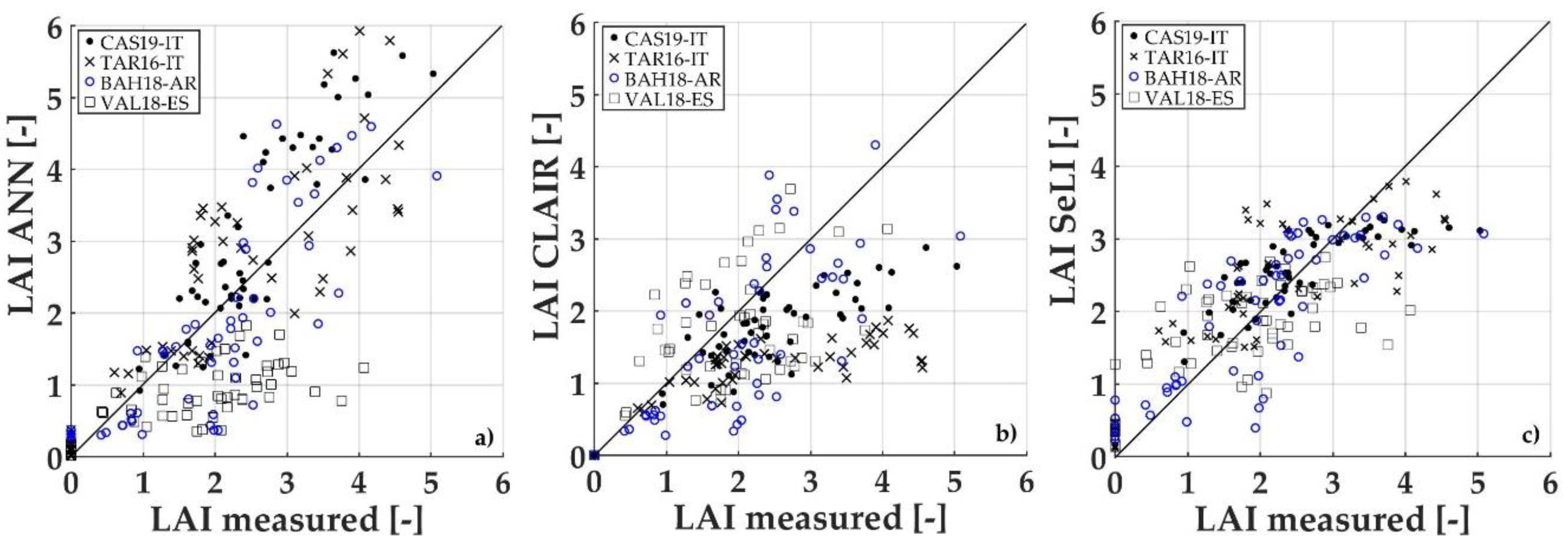
3.1. Performance of LAI Estimation Methods

For the application of the CLAIR model, two methods for α* estimation were applied. In the first approach, simply named CLAIR, a fixed reference value for α* was applied depending on the two general crop types (0.41 for herbaceous crops and 0.30 for tree crops). In a second approach, named CLAIR_opt, a calibrated α* value was applied from S2 image for each study area. The calibration consists of a regression analysis technique applied to the observed and CLAIR estimated LAI values of the satellite image where there are more in situ values. The resulting calibrated α* is considered the new constant α* and it is used in the rest of the images of the corresponding study area.

Table 5. Soil line slope, ${\mathrm{WDVI}}_{\infty }$ and calibrated extinction coefficient (α*) values used in the Clevers leaf area index by reflectance (CLAIR) model obtained for each satellite image in each test site. The satellite image used to calibrate α* is boldfaced.

Test Site	Acquisition Dates	Soil Line Slope	${\mathbf{WDVI}}_{\infty }$	α* (Calibrated)
CAS19_IT	March 09, 2019	0.990	0.728	0.27
	March 19, 2019	0.986	0.784	0.27
TAR16_IT	March 17, 2016	0.984	0.943	0.20
	April 19, 2016	0.983	0.971	0.20
	May 06, 2016	0.993	1.026	0.20
	June 08, 2016	0.978	0.927	0.20
	June 25, 2016	0.999	0.917	0.20
	July 08, 2016	0.995	0.788	0.20
	July 28, 2016	0.995	0.774	0.20
BAH18_AR	November 18, 2018 (T20 HNB)	0.984	0.590	0.69
	November 18, 2018 (T20 HNC)	0.989	0.534	0.69
	November 23, 2018 (T20 HNB)	0.985	0.571	0.69
VAL18_ES	October 03, 2018	0.998	0.519	0.58 (herb. crops) 0.27 (tree crops)

specifies the values obtained for soil line slope, ${\mathrm{WDVI}}_{\infty }$ and α* calibrated for each of the study areas.

The ANN S2 product, CLAIR model, CLAIR_opt model and the different VIs for LAI estimation were obtained for each test site and compared with the corresponding in situ LAI values of each dataset.

Table 6. Statistics (R² and root mean square error, RMSE) obtained between each model and LAI in situ values, with linear fitting. The best result for each study site is boldfaced, prioritizing the RMSE.

Model		CAS19_IT		TAR16_IT		BAH18_AR		VAL18_ES		All Datasets
		R2	RMSE	R2	RMSE	R2	RMSE	R2	RMSE	R2	RMSE
ANN S2		0.863	0.79	0.742	0.86	0.702	0.78	0.473	1.19	0.639	0.92
CLAIR		0.798	0.90	0.715	1.47	0.631	0.86	0.460	0.84	0.529	1.04
CLAIRopt		0.800	0.60	0.712	0.78	0.631	1.22	0.460	0.93	0.576	0.91
VI	RVI	0.802	0.56	0.433	1.09	0.493	0.90	0.346	0.86	0.540	0.87
	NDVI	0.736	0.65	0.696	0.80	0.714	0.68	0.525	0.73	0.689	0.71
	NDI	0.709	0.68	0.605	0.91	0.640	0.76	0.369	0.85	0.610	0.80
	RENDVI	0.782	0.59	0.478	1.05	0.609	0.85	0.217	0.94	0.542	0.87
	SeLI	0.805	0.56	0.709	0.78	0.721	0.67	0.468	0.78	0.702	0.70
	TRBI	0.710	0.68	0.673	0.83	0.719	0.67	0.523	0.74	0.677	0.73
	IRECI	0.852	0.49	0.655	0.85	0.605	0.80	0.437	0.80	0.662	0.75
	EVI	0.802	0.56	0.744	0.74	0.673	0.72	0.520	0.74	0.708	0.69

summarizes the different statistics (R² and RMSE) obtained for each test site, being the p-value < 0.001 in all cases. In general, almost all models produced results that came close to the ground-truth (R² > 0.6, RMSE < 0.9), except in the case of the Valencia dataset where all models obtained worse statistics, R² < 0.6 and a RMSE > 0.7. This may be due to the fact that this study area is mainly composed of crop types, e.g., lettuce, onion and orange tree which have a scarce and dispersed coverage, translating into a strong soil influence. Additionally, it is shown how the CLAIR_opt model results are similar to those obtained with the non-calibrated model, improving slightly in the CAS19_IT and TAR16_IT dataset, i.e., halving the RMSE. In the two other datasets, the results of the CLAIR_opt model are worse than the CLAIR model with fixed values. This may be because α* is optimized with only one satellite image per test site, which has the highest number of in situ values, making in some cases a possible error in α* creating a large impact on the results.

The results of each model for all four study sites together are shown in Figure 3. Figure 3a represents the validation of ANN S2 LAI product, observing that all the data are close to 1:1 line, except for the LAI in situ data from Valencia, where the ANN LAI product underestimates the LAI values (Table 6, RMSE = 1.19). Figure 3b shows the LAI values obtained with the CLAIR model with fixed values. In this case, the LAI values are more dispersed, being the LAI estimated values corresponding to the Tarquinia study area the least close to the in situ values (Table 6, RMSE = 1.47). Finally, Figure 3c shows the LAI values estimated with the SeLI index together with the different in situ data (LAI = 4.885SeLI − 0.205). The SeLI index is an index that presents good statistics in the different datasets, hence, the reason for its selection. Observing the graph, the LAI values are less dispersed but a clear saturation of the estimated LAI values with LAI values greater than 4 can be distinguished. The ANN S2 LAI product is the retrieval methodology that presents the least saturation problems with high LAI values.

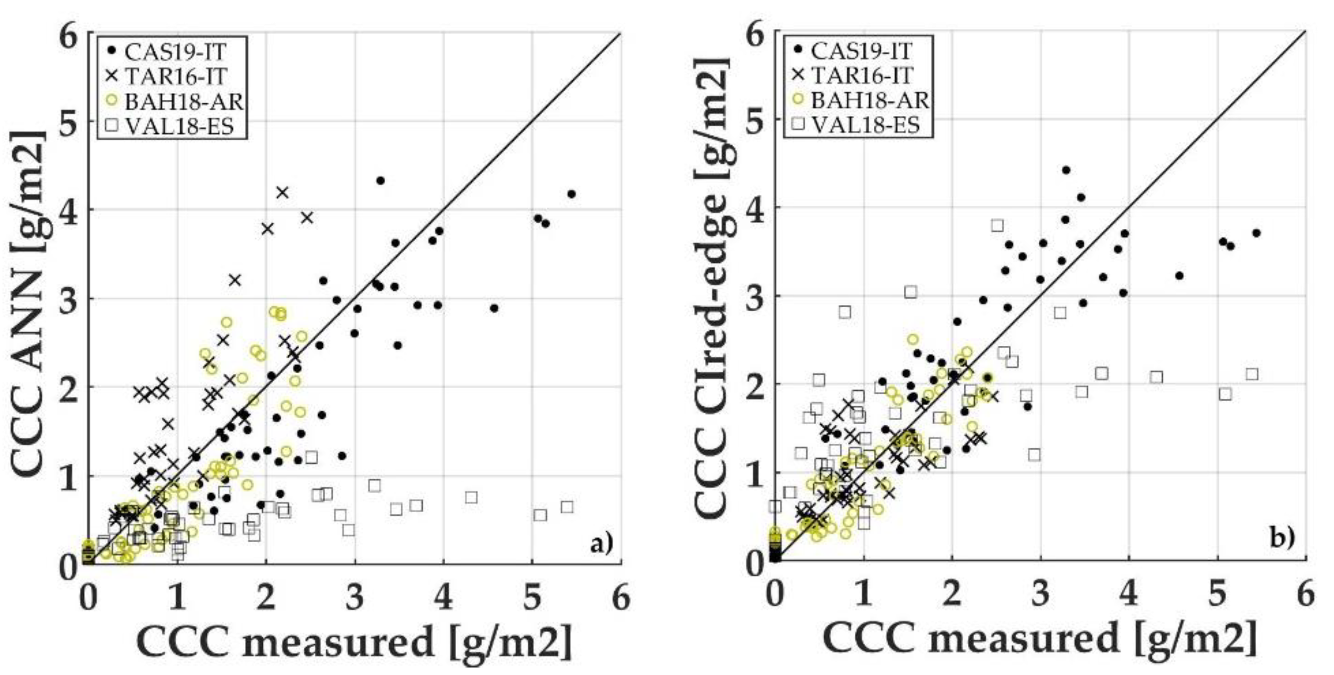
3.2. Performance of CCC Estimation Methods

In the case of the CCC variable, the ANN S2 CCC product and the VIs most widely used by the bibliography for CCC retrieval were calculated.

Table 7. Statistics (R² and RMSE) obtained between each model and CCC in situ values, with linear fitting. The best result for each study site is boldfaced, prioritizing the RMSE.

Model		CAS19_IT		TAR16_IT		BAH18_AR		VAL18_ES		All Datasets
		R2	RMSE (g/m2)	R2	RMSE (g/m2)	R2	RMSE (g/m2)	R2	RMSE (g/m2)	R2	RMSE (g/m2)
ANN S2		0.847	0.68	0.775	0.67	0.745	0.45	0.473	1.45	0.502	0.89
VI	CIred-edge	0.806	0.62	0.667	0.40	0.827	0.32	0.408	0.99	0.710	0.64
	CIgreen	0.794	0.64	0.712	0.37	0.802	0.34	0.427	0.98	0.712	0.63
	TCARI	0.813	0.61	0.543	0.47	0.754	0.38	0.182	1.16	0.628	0.72
	OSAVI	0.684	0.79	0.582	0.45	0.819	0.32	0.315	1.07	0.630	0.72
	MTCI	0.705	0.76	0.569	0.46	0.777	0.36	0.371	1.06	0.637	0.71
	NDRE1	0.679	0.80	0.603	0.44	0.822	0.32	0.376	1.02	0.649	0.70
	NDRE2	0.690	0.78	0.639	0.42	0.831	0.31	0.422	0.98	0.670	0.68
	NAOC	0.627	0.86	0.609	0.43	0.803	0.34	0.384	1.01	0.631	0.72

shows the statistics obtained by applying both methodologies at each study site, being the p-value < 0.001 in all cases. The different CCC methods present similar results to those obtained for the LAI parameter. Almost all models present good statistics (R² > 0.5, RMSE < 0.8 g/m²) in comparison with in situ CCC values, with only the Valencia test site presenting worse statistics (R² < 0.5, RMSE > 0.9 g/m²). Eight VIs widely used in literature for the estimation of the CCC parameter were tested, being the CI_red-edge one of the best indices in each of the datasets.

Figure 4 shows the in situ CCC values together with the values estimated using CI_red-edge index and ANN S2 CCC product. Figure 4a shows the CCC values obtained with the ANN S2 CCC product, with a behaviour similar to that obtained with the ANN S2 LAI product, i.e., the values are close to 1:1 line, except for those corresponding to the Valencia dataset, in which there is a clear underestimation in comparison with the in situ values. Figure 4b, on the other hand, shows the CCC values estimated with the CI_red-edge index, which is the index that presents good statistics in the different datasets (CCC (g/m²) = 0.522CI_red-edge + 0.198). In this case, the CI_red-edge index does not produce as much saturation as the SeLI index (Figure 3c), with the CCC values approaching the 1:1 line, except in the case of the Valencia study area where the CCC values are still underestimated.

3.3. Impact of LAI Uncertainty on the Estimation of ETc in Irrigated Crops

Given the different LAI retrieval methodologies, this study applied the FAO-56 PM equation (Equation (7)) to estimate the ET_c of the wheat and tomato crop types in the seasonal dataset from Tarquinia (Italy) (Figure 5). Specifically, ET_c was calculated with both the albedo and LAI retrievals, estimated from the S2 images, together with the specific climatic conditions. In addition, the ET_c values obtained with the traditional reference evapotranspiration (ET_o) methodology by the corresponding crop-based K_c coefficient (ET_o × K_c in black) were added. Specifically, a constant K_c value of 1.15 was used for the wheat crop type and for tomato, first 1.15 and in the late season stage of the plant (end of July), a value of 0.8. In the absence of the reference and independent ET data, i.e., from an Eddy Covariance station, the estimated ET_c with the LAI in situ values were considered as the proxy of the ground-truth ET_c (in red). The error bars are also included in Figure 5, corresponding with the standard deviation obtained within each ESU that composes the TAR16_IT dataset. The ET_o × K_c method does not present error bars because for the whole wheat and tomato plot, it presents the same value without differences.

Figure 5a,b show the short-seasonal trend of ET_c for wheat (March to May) and tomato (May to July), respectively.

Table 8. Statistics (R² and RMSE) obtained between ET_c estimated with LAI in situ and ET_c estimated with each of the models, with linear fitting. The best results are boldfaced.

	WHEAT		TOMATO
Model	ETc LAI In Situ
	R2	RMSE (mm/d)	R2	RMSE (mm/d)
ETo × Kc	0.998	0.32	0.240	1.17
ETc ANN LAI S2	0.902	0.41	0.971	0.33
ETc LAI CLAIR	0.978	1.42	0.985	1.10
ETc LAI SeLI	0.998	0.31	0.672	0.54

specifies the R² and RMSE between ET_c obtained by the different LAI retrievals and ET_c obtained by in situ LAI data, being the p-value < 0.001 in all cases. Observing Figure 5a, together with the values in Table 8, the ET_c estimated with the LAI values of the SeLI index are the closest to the ET_c values obtained with LAI in situ (R² = 0.998, RMSE = 0.31 mm/d), followed by the ET_o × K_c method (R² = 0.998, RMSE = 0.32 mm/d) and the ET_c estimated with ANN S2 LAI product (R² = 0.902, RMSE = 0.41 mm/d). On the other hand, in Figure 5b, this study identified that the ET_c values closest to those estimated with LAI in situ, are the ones obtained with the ANN S2 LAI product (R² = 0.971, RMSE = 0.33 mm/d), followed by ET_c estimated with the SeLI index (R² = 0.672, RMSE = 0.54 mm/d). In this case, the ET_c estimated with the ET_o × K_c method presents statistics that can be improved (R² = 0.240, RMSE = 1.17 mm/d). In both crop types, the ET_c estimated with LAI CLAIR presents a high RMSE, greater than 1 mm/d, according to the results obtained previously (Table 6).

4. Discussion

The importance of estimating biophysical variables lies in their use as input parameters for various models dedicated to the monitoring of seasonal plant functioning and the optimization of agricultural zones. If the estimation of variables, such as LAI and CCC, is through satellites as S2, information of these key variables can be obtained with high frequency and spatial resolution, increasing the accuracy of the dynamical models fed by their input. This study analyzes different methodologies to estimate LAI and CCC, the essential parameters for the understanding of the evapotranspiration process. Specifically, empirical (VIs), semi-empirical (CLAIR model with fixed and calibrated extinction coefficient) and ANN S2 products are derived from SNAP biophysical processor approaches for the LAI and CCC estimation, using S2 spectral information. Previous S2 retrieval works are commonly based on simulated data [68] or on in situ data taken only in one test site [69]. The main strength of this study is the use of four datasets with in situ multi-crop information obtained with different instruments from totally diverse test sites.

The VIs most commonly used by the scientific community for the LAI and CCC remote retrieval were applied to the four study areas. These indices have produced good results in previous studies both in the analysis of a single crop type [54,58] and in the studies with a variety of crops [55,63,70]. In this study, one of the best indices, together with the EVI index, for the estimation of LAI in the four datasets i.e., successful in multi-crop data, was the SeLI index. This is a consistent result with a previous work that was done with LAI data taken in a multi-crop area [33]. SeLI uses the red-edge region as the area of greatest influence of the LAI (B5—705 nm) and the NIR region as the control band (B8a—865 nm). Furthermore, for the estimation of the CCC parameter, one of the VI with the best statistics in each dataset is the CI_red-edge, which uses a two bands ratio located in the red-edge region (B5—705 nm, B7—783 nm). The S2 bands located in the red-edge area have been identified as key bands for the biophysical parameters estimation, mainly the LAI [52] and CCC [71]. One of the main critics of VIs is that it does not take into account other parameters that affect reflectance [16]. Hence, the methodologies based on VIs have been developed and improved by incorporating the calibration factors, such as the influence of bare soil. This is the case of the semi-empirical CLAIR [22] model composed of the WDVI, soil line concept and a correction coefficient corresponding to the minimum error between the observed and estimated LAI (α*). This model has been widely used for the estimation of the LAI parameter with different satellites such as DEIMOS-1 [72] or WorldView-2 [73], and even with the S2 satellite [74]. In this study, this model is first estimated with a fixed value of α* parameter and after being checked with an optimized α* for each test site. The results with the optimized CLAIR model (CLAIR_opt) are better in the CAS19_IT and TAR16_IT datasets, especially in the latter where RMSE is halved. However, the CLAIR_opt model obtains worse results in the Bahía Blanca and Valencia test areas. This may be due to the fact that the fixed value of α* is 0.41 and the optimized value is approximately 0.30 for the image with the highest number of in situ points. However, if the optimized α* of another image is checked, it returns approximately 0.60, so 0.41 is an intermediate value, obtaining in the end better results with the non-optimized CLAIR model. Other studies have obtained also better results with a fixed α* value than by performing a calibration process [72]. Therefore, from an operational point of view, the CLAIR model can be used with constant values. In case the area of study is specific, a calibration can be made but it should include the maximum in situ points from several images for an optimal calibration. On the other hand, several authors who have used the CLAIR model in their studies obtained saturation problems with high LAI values when WDVI value tended to ${\mathrm{WDVI}}_{\infty }$ [75]. This saturation process also occurs in our four datasets with the LAI values higher than 3. Generally, the studies based on the CLAIR model visually select approximately 50–100 bare soil pixels in the satellite image to estimate the soil line slope [72]. In this case, the soil line slope value has been estimated from all the bare soil pixels in the image, masking the rest of the pixels. In this case, the SCL map derived by Sen2Cor have been used for masking, producing good results.

Regarding the ANN S2 LAI and CCC products, the LAI product has been validated in several studies, obtaining results that can be improved (R² = 0.5), both when applied to a single crop type [76] and when validated with multi-crop data [33]. Even studies that have carried out an analysis of different retrieval methodologies concluded that VIs produce better results than the ANN S2 LAI product [77]. In this study, the ANN S2 LAI product obtains good results in the three datasets corresponding to Caserta, Tarquinia and Bahía Blanca test sites (R² > 0.7, RMSE < 0.9 g/m²). The validation of the ANN S2 CCC product, on the other hand, has been done by very few studies and only for the wheat crop type. These studies obtained good results. A recent study [76] obtained a R² = 0.72 with the ANN S2 CCC product and in situ wheat data, and [78] has defined a relation between the ANN S2 CCC product and the canopy nitrogen, obtaining a R² = 0.90. The results of this study support and extend these results, obtaining a R² > 0.7 and RMSE < 0.7 g/m², for three totally different agricultural areas and with different crop types: Caserta, Tarquinia and Bahía Blanca test sites.

The special case of the Valencia study area should be mentioned. This study site is characterized by very small plots (40–100 m in length) and composed of some crop types (e.g., orange tree and lettuce) with a fraction vegetation cover (FVC) ≈ 50% [33], leaving the soil an important role. Therefore, the VIs and the ANN S2 products do not present good statistics in this area. The CLAIR model includes a soil correction factor, the soil line slope concept, which is expected to present better statistics. However, the model obtains improvable statistics (R² = 0.46, RMSE = 0.84). The FVC has always influenced remote sensing studies, not only in the biophysical retrieval models, also in studies related to evapotranspiration and irrigation management [79,80]. Therefore, it is necessary to incorporate the FVC parameter in the biophysical models, mainly when they are applied to areas such as Valencia. A possible solution is to use the ANN S2 FVC product, but this must be validated to a further extent as very few studies are available concerning the quality analysis of this product. For example, a recent study [77] has validated the ANN S2 FVC product in soybeans, canola, wheat, corn, oats, black beans and alfalfa crop types, obtaining good results.

In general, the Plant Canopy Analyzer (LAI-2000, LAI-2200) is the instrument most commonly used to measure in situ LAI parameter [81,82]. However, in many cases, this instrument is not available due to its high cost. In this study, the LAI data from Caserta, Tarquinia and Valencia were taken with the standard LAI instrument but the Bahía Blanca (Argentina) data were obtained with the PocketLAI smartphone application [83]. This application has been used in several previous works with satisfactory results, mainly on rice crop studies [84,85] but also on other crop types such as vineyards [86]. In this last study [86], both PocketLAI and the digital hemispherical photography (DHP) instrument were used and compared with destructive LAI values, observing that PocketLAI measurements were closer to the ground-truth (RRMSE = 43.00% for PocketLAI; RRMSE = 99.46% for DHP). Furthermore, in a recent comparative study of different LAI measurement instruments against destructive LAI values [39], the PocketLAI was found to a good alternative for the LAI operational measurement due to its cost-effective and similar results to destructive LAI values, obtaining a RMSE of < 0.65 for alfalfa, broad bean and maize crop types.

Finally, the influence of the biophysical parameter retrieval methodologies over the biophysical model outputs was analyzed. Crop potential evapotranspiration (ET_c) has been estimated using the FAO-56 PM equation adapted to remote sensing [3]. In general, the ET_c is estimated using the reference evapotranspiration (ET_o) by a crop specific coefficient (K_c), focusing the different studies on optimizing this coefficient for the different crop types with satellite data. For example, [5] optimized the K_c coefficient for wheat using SPOT-4 satellite data and [7] optimized the K_c coefficient for vineyards with Landsat 8—RapidEye satellite data combination. In this study, on the other hand, the standard K_c values established by FAO [3] for each crop type and growth stage were selected and the impact of the LAI parameter on the model was analyzed. The LAI obtained with the different methodologies was used as an input. As a result, the ET_c estimated with the ANN S2 LAI product is the closest to the ET_c estimated with the in situ LAI. Previous satellite evapotranspiration estimation studies have also used the ANN S2 LAI product as an input, producing satisfactory results in comparison with the soil water balance module in the environmental policy integrated climate (EPIC) model [64]. In addition, this study found that the satellite retrieved LAI values provided a more pronounced seasonal trend compared to the K_c approach for both wheat and tomato crop types.

In short, the ANN S2 products are the closest match to the in situ data. From the operational point of view, this study provides evidence that ANN S2 LAI and CCC products have great potential to be used for the estimation and understanding of evapotranspiration, being one of the methodologies that provide similar results to ground-truth, without saturation problems. In future works, the authors want to validate the ANN S2 FVC product with the objective of incorporating this parameter in models applied to the study areas with low vegetation cover FVC ≤ 50%, as is the case of Valencia area.

5. Conclusions

This study performs a comparative analysis of commonly used methods, vegetation indices (VIs), CLAIR model and artificial neural network Sentinel-2 biophysical processor products (ANN S2 products), for the estimation of leaf area index (LAI) and canopy chlorophyll content (CCC) using the S2 satellite spectral information. Both parameters are essential for the estimation and understanding of the evapotranspiration process. The main strength of this study is that it is based on four in situ LAI and CCC datasets obtained in different parts of the world (Argentina, Italy and Spain), with diverse instruments, from standard instruments (LAI-2000, SPAD) to smartphone applications such as PocketLAI. By applying the methodologies to the different datasets, the ANN S2 products produced good retrieval results both for the LAI (R² > 0.70, RMSE < 0.86) and for the CCC (R² > 0.75, RMSE < 0.68 g/m²) parameter. Regarding VIs, the normalized SeLI index is the one that obtains the best results in the different datasets for LAI retrieval and for the CCC, the CI_red-edge ratio index. Both indices use bands located in the red-edge zone, highlighting the importance of this region. On the other hand, the CLAIR model estimated with fixed extinction values (α*) of 0.41 for herbaceous crops and 0.30 for tree species obtained good statistics (R² > 0.63, RMSE < 1.47) and the CLAIR model optimizing the parameter α* (CLAIR_opt) for each of the study areas only slightly improved the RMSE in the two Italian datasets (RMSE ≈ 0.70). It should be mentioned that with the Valencia area dataset, all the methodologies produce statistics that can be improved, due to the high soil influence in this area and the small size of the plots (< 1 ha). Finally, the influence of the LAI parameter on the FAO-56 PM evapotranspiration model adapted to remote sensing was analyzed. This analysis showed that the crop potential evapotranspiration (ET_c) values estimated with the ANN S2 LAI product are the closest to those estimated with the in situ LAI values (R² > 0.90, RMSE < 0.41 mm/d) using a dataset with seasonal information of wheat and tomato. Therefore, with all the above, it can be concluded that VIs produce the best statistics, but the ANN S2 products are the only ones that do not produce saturation, demonstrating the great potential of ANN S2 products for operational use in the monitoring of agricultural areas.

References

1. Brisco, B.; Brown, R.J.; Hirose, T.; McNairn, H.; Staenz, K. Precision agriculture and the role of remote sensing: A review. Can. J. Remote Sens. 1998, 24, 315–327. [Google Scholar] [CrossRef]
2. Wang, K.; Franklin, S.E.; Guo, X.; Cattet, M. Remote sensing of ecology, biodiversity and conservation: A review from the perspective of remote sensing specialists. Sensors 2010, 10, 9647–9667. [Google Scholar] [CrossRef] [PubMed]
3. Allen, R.G.; Pereira, L.S.; Raes, D.; Smith, M. Crop Evapotranspiration—Guidelines for Computing Crop Water Requirements; Food and Agriculture Organization of the United Nations: Rome, Italy, 1998; Volume 300. [Google Scholar]
4. D’Urso, G. Current status and perspectives for the estimation of crop water requirements from earth observation. Ital. J. Agron. 2010, 5, 107–120. [Google Scholar] [CrossRef]
5. Farg, E.; Arafat, S.M.; Abd El-Wahed, M.S.; El-Gindy, A.M. Estimation of evapotranspiration ETc and crop coefficient Kc of wheat, in south Nile Delta of Egypt using integrated FAO-56 approach and remote sensing data. Egypt. J. Remote Sens. Sp. Sci. 2012, 15, 83–89. [Google Scholar] [CrossRef]
6. Glenn, E.P.; Neale, C.M.U.; Hunsaker, D.J.; Nagler, P.L. Vegetation index-based crop coefficients to estimate evapotranspiration by remote sensing in agricultural and natural ecosystems. Hydrol. Process. 2011, 25, 4050–4062. [Google Scholar] [CrossRef]
7. Vanino, S.; Pulighe, G.; Nino, P.; de Michele, C.; Bolognesi, S.F.; D’Urso, G. Estimation of evapotranspiration and crop coefficients of tendone vineyards using multi-sensor remote sensing data in a mediterranean environment. Remote Sens. 2015, 7, 14708–14730. [Google Scholar] [CrossRef]
8. Chen, J.M.; Black, T.A. Defining leaf area index for non-flat leaves. Plant. Cell Environ. 1992, 15, 421–429. [Google Scholar] [CrossRef]
9. Delegido, J.; Van Wittenberghe, S.; Verrelst, J.; Ortiz, V.; Veroustraete, F.; Valcke, R.; Samson, R.; Rivera, J.P.; Tenjo, C.; Moreno, J. Chlorophyll content mapping of urban vegetation in the city of Valencia based on the hyperspectral NAOC index. Ecol. Indic. 2014, 40, 34–42. [Google Scholar] [CrossRef]
10. Gitelson, A.A.; Viña, A.; Verma, S.B.; Rundquist, D.C.; Arkebauer, T.J.; Keydan, G.; Leavitt, B.; Ciganda, V.; Burba, G.G.; Suyker, A.E. Relationship between gross primary production and chlorophyll content in crops: Implications for the synoptic monitoring of vegetation productivity. J. Geophys. Res. Atmos. 2006, 111, 1–13. [Google Scholar] [CrossRef]
11. Boegh, E.; Soegaard, H.; Broge, N.; Hasager, C.B.; Jensen, N.O.; Schelde, K.; Thomsen, A. Airborne multispectral data for quantifying leaf area index, nitrogen concentration, and photosynthetic efficiency in agriculture. Remote Sens. Environ. 2002, 81, 179–193. [Google Scholar] [CrossRef]
12. Gianquinto, G.; Orsini, F.; Fecondini, M.; Mezzetti, M.; Sambo, P.; Bona, S. A methodological approach for defining spectral indices for assessing tomato nitrogen status and yield. Eur. J. Agron. 2011, 35, 135–143. [Google Scholar] [CrossRef]
13. Houlès, V.; Guérif, M.; Mary, B. Elaboration of a nitrogen nutrition indicator for winter wheat based on leaf area index and chlorophyll content for making nitrogen recommendations. Eur. J. Agron. 2007, 27, 1–11. [Google Scholar] [CrossRef]
14. Solari, F.; Shanahan, J.; Ferguson, R.; Schepers, J.; Gitelson, A. Active sensor reflectance measurements of corn nitrogen status and yield potential. Agron. J. 2008, 100, 571–579. [Google Scholar] [CrossRef]
15. Sakamoto, T.; Gitelson, A.; Nguy-Robertson, A.; Arkebauer, T.; Wardlow, B.; Suyker, A.; Verma, S.; Shibayama, M. An alternative method using digital cameras for continuous monitoring of crop status. Agric. For. Meteorol. 2012, 154, 113–126. [Google Scholar] [CrossRef]
16. Daughtry, C.S.T.; Walthall, C.L.; Kim, M.S.; De Colstoun, E.B.; McMurtrey, J.E. Estimating corn leaf chlorophyll concentration from leaf and canopy reflectance. Remote Sens. Environ. 2000, 74, 229–239. [Google Scholar] [CrossRef]
17. Gitelson, A.A.; Viña, A.; Ciganda, V.; Rundquist, D.C.; Arkebauer, T.J. Remote estimation of canopy chlorophyll content in crops. Geophys. Res. Lett. 2005, 32, 1–4. [Google Scholar] [CrossRef]
18. Weiss, M.; Baret, F.; Myneni, R.; Pragnère, A.; Knyazikhin, Y. Investigation of a model inversion technique for the estimation of crop characteristics from spectral and directional reflectance data. Agronomie 2000, 20, 3–22. [Google Scholar] [CrossRef]
19. Bréda, N.J.J. Ground-based measurements of leaf area index: A review of methods, instruments and current controversies. J. Exp. Bot. 2003, 54, 2403–2417. [Google Scholar] [CrossRef]
20. Yao, X.; Wang, N.; Liu, Y.; Cheng, T.; Tian, Y.; Chen, Q.; Zhu, Y. Estimation of wheat LAI at middle to high levels using unmanned aerial vehicle narrowband multispectral imagery. Remote Sens. 2017, 9, 1304. [Google Scholar] [CrossRef]
21. Campos-Taberner, M.; García-Haro, F.J.; Camps-Valls, G.; Grau-Muedra, G.; Nutini, F.; Crema, A.; Boschetti, M. Multitemporal and multiresolution leaf area index retrieval for operational local rice crop monitoring. Remote Sens. Environ. 2016, 187, 102–118. [Google Scholar] [CrossRef]
22. Clevers, J.G.P.W. The application of a weighted infrared-red vegetation index for estimating leaf area index by correcting for soil moisture. Remote Sens. Environ. 1989, 29, 25–37. [Google Scholar] [CrossRef]
23. Lázaro-gredilla, M.; Titsias, M.K.; Verrelst, J.; Camps-valls, G.; Member, S. Retrieval of biophysical parameters with heteroscedastic gaussian processes. IEEE Geosci. Remote Sens. Lett. 2013, 11, 838–842. [Google Scholar] [CrossRef]
24. Bacour, C.; Baret, F.; Béal, D.; Weiss, M.; Pavageau, K. Neural network estimation of LAI, fAPAR, fCover and LAI×Cab, from top of canopy MERIS reflectance data: Principles and validation. Remote Sens. Environ. 2006, 105, 313–325. [Google Scholar] [CrossRef]
25. Casa, R.; Baret, F.; Buis, S.; Lopez-Lozano, R.; Pascucci, S.; Palombo, A.; Jones, H.G. Estimation of maize canopy properties from remote sensing by inversion of 1-D and 4-D models. Precis. Agric. 2010, 11, 319–334. [Google Scholar] [CrossRef] [Green Version]
26. Frederic, B.; Buis, S. Estimating canopy characteristics from remote sensing observations: Review of methods and associated problems. In Advances in Land Remote Sensing; Springer: Berlin, Germany, 2008; pp. 173–201. ISBN 978-1-4020-6449-4. [Google Scholar]
27. Atzberger, C. Object-based retrieval of biophysical canopy variables using artificial neural nets and radiative transfer models. Remote Sens. Environ. 2004, 93, 53–67. [Google Scholar] [CrossRef]
28. Mulla, D.J. Twenty five years of remote sensing in precision agriculture: Key advances and remaining knowledge gaps. Biosyst. Eng. 2013, 114, 358–371. [Google Scholar] [CrossRef]
29. Bisquert, M.; Sánchez, J.M.; López-Urrea, R.; Caselles, V. Estimating high resolution evapotranspiration from disaggregated thermal images. Remote Sens. Environ. 2016, 187, 423–433. [Google Scholar] [CrossRef]
30. Drusch, M.; Del Bello, U.; Carlier, S.; Colin, O.; Fernandez, V.; Gascon, F.; Hoersch, B.; Isola, C.; Laberinti, P.; Martimort, P.; et al. Sentinel-2: ESA’s optical high-resolution mission for GMES operational services. Remote Sens. Environ. 2012, 120, 25–36. [Google Scholar] [CrossRef]
31. Weiss, M.; Baret, F. S2ToolBox Level 2 Products: LAI, FAPAR, FCOVER. Available online: http://step.esa.int/docs/extra/ATBD_S2ToolBox_L2B_V1.1.pdf (accessed on 29 July 2019).
32. Djamai, N.; Fernandes, R. Comparison of SNAP-derived Sentinel-2A L2A product to ESA product over Europe. Remote Sens. 2018, 10, 926. [Google Scholar] [CrossRef]
33. Pasqualotto, N.; Delegido, J.; Van Wittenberghe, S.; Rinaldi, M.; Moreno, J. Multi-crop green LAI estimation with a new simple Sentinel-2 LAI Index (SeLI). Sensors 2019, 19, 904. [Google Scholar] [CrossRef]
34. METEOBLUE Weather. Climate Caserta. Available online: https://www.meteoblue.com/en/weather/forecast/modelclimate/caserta_italy_3179866 (accessed on 15 May 2019).
35. METEOBLUE Weather. Climate Tarquinia. Available online: https://www.meteoblue.com/en/weather/forecast/modelclimate/tarquinia_italy_3165919 (accessed on 15 May 2019).
36. METEOBLUE Weather. Climate Bahía Blanca. Available online: https://www.meteoblue.com/en/weather/forecast/modelclimate/bahía-blanca_argentina_3865086 (accessed on 15 May 2019).
37. METEOBLUE Weather. Climate Valencia. Available online: https://www.meteoblue.com/en/weather/forecast/modelclimate/valencia_spain_2509954 (accessed on 15 May 2019).
38. VALERI. Land European Remote-Sensing Instruments Field Protocol. Available online: http://w3.avignon.inra.fr/valeri/ (accessed on 16 May 2019).
39. Casa, R.; Upreti, D.; Pelosi, F. Measurement and estimation of leaf area index (LAI) using commercial instruments and smartphone-based systems. IOP Conf. Ser. Earth Environ. Sci. 2019, 275, 012006. [Google Scholar] [CrossRef]
40. Parry, C.; Mark Blonquist, J.; Bugbee, B. In situ measurement of leaf chlorophyll concentration: Analysis of the optical/absolute relationship. Plant. Cell Environ. 2014, 37, 2508–2520. [Google Scholar] [CrossRef] [PubMed]
41. European Space Agency (ESA). ESA’s Optical High-Resolution Mission for GMES Operational Services. Available online: https://sentinel.esa.int/documents/247904/349490/S2_SP-1322_2.pdf (accessed on 29 July 2019).[Green Version]
42. ESA server. Available online: https://scihub.copernicus.eu/ (accessed on 3 May 2019).
43. Louis, J.; Debaecker, V.; Pflug, B.; Main-Knorn, M.; Bieniarz, J.; Mueller-Wilm, U.; Cadau, E.; Gascon, F. Sentinel-2 SEN2COR: L2A processor for users. In Proceedings of the Living Planet Symposium, Prague, Czech Republic, 9–13 May 2016; pp. 1–8. [Google Scholar]
44. Jacquemoud, S.; Baret, F. PROSPECT: A model of leaf optical properties spectra. Remote Sens. Environ. 1990, 34, 75–91. [Google Scholar] [CrossRef]
45. Verhoef, W. Light scattering by leaf layers with application to canopy reflectance modeling: The SAIL model. Remote Sens. Environ. 1984, 16, 125–141. [Google Scholar] [CrossRef] [Green Version]
46. Baret, F.; Jacquemoud, S.; Hanocq, J.F. About the soil line concept in remote sensing. Adv. Sp. Res. 1993, 13, 281–284. [Google Scholar] [CrossRef]
47. Vuolo, F.; Dini, L.; D’Urso, G. Assessment of LAI retrieval accuracy by inverting a RT model and a simple empirical model with multiangular and hyperspectral CHRIS/PROBA data from SPARC. In Proceedings of the 3rd CHRIS/Proba Workshop, Frascati, Italy, 21–23 March 2005. [Google Scholar]
48. Akdim, N.; Alfieri, S.M.; Habib, A.; Choukri, A.; Cheruiyot, E.; Labbassi, K.; Menenti, M. Monitoring of irrigation schemes by remote sensing: Phenology versus retrieval of biophysical variables. Remote Sens. 2014, 6, 5815–5851. [Google Scholar] [CrossRef]
49. Fox, G.A.; Sabbagh, G.J.; Searcy, S.W.; Yang, C. An automated soil line identification routine for remotely sensed images. Soil Sci. Soc. Am. J. 2004, 68, 1326. [Google Scholar] [CrossRef]
50. Jordan, C.F. Derivation of leaf area index from quality of light on the forest floor. Ecology 1969, 50, 663–666. [Google Scholar] [CrossRef]
51. Rouse, J.W.; Hass, R.H.; Schell, J.A.; Deering, D.W. Monitoring vegetation systems in the great plains with ERTS. In Proceedings of the Third Earth Resources Technology Satellite (ERTS) Symposium, Washington, DC, USA, 10–14 December 1973; Volume 1, pp. 309–317. [Google Scholar]
52. Delegido, J.; Verrelst, J.; Alonso, L.; Moreno, J. Evaluation of sentinel-2 red-edge bands for empirical estimation of green LAI and chlorophyll content. Sensors 2011, 11, 7063–7081. [Google Scholar] [CrossRef]
53. Sharma, L.K.; Bu, H.; Denton, A.; Franzen, D.W. Active-optical sensors using red NDVI compared to red edge NDVI for prediction of corn grain yield in North Dakota, U.S.A. Sensors 2015, 15, 27832–27853. [Google Scholar] [CrossRef]
54. Vincini, M.; Frazzi, E.; D’Alessio, P. Comparison of narrow-band and broad-band vegetation indices for canopy chlorophyll density estimation in sugar beet. In Proceedings of the 6th European Conference on Precision Agriculture, Skiathos, Greece, 3–6 June 2007; pp. 189–196. [Google Scholar]
55. Frampton, W.J.; Dash, J.; Watmough, G.; Milton, E.J. Evaluating the capabilities of Sentinel-2 for quantitative estimation of biophysical variables in vegetation. ISPRS J. Photogramm. Remote Sens. 2013, 82, 83–92. [Google Scholar] [CrossRef] [Green Version]
56. Huete, A.; Didan, K.; Miura, T.; Rodriguez, E.P.; Gao, X.; Ferreira, L.G. Overview of the radiometric and biophysical performanceof the MODIS vegetation indices. Remote Sens. Environ. 2002, 83, 195–213. [Google Scholar] [CrossRef]
57. Gitelson, A.A.; Gritz, Y.; Merzlyak, M.N. Relationships between leaf chlorophyll content and spectral reflectance and algorithms for non-destructive chlorophyll assessment in higher plant leaves. J. Plant Physiol. 2003, 160, 271–282. [Google Scholar] [CrossRef] [PubMed]
58. Haboudane, D.; Miller, J.R.; Tremblay, N.; Zarco-Tejada, P.J.; Dextraze, L. Integrated narrow-band vegetation indices for prediction of crop chlorophyll content for application to precision agriculture. Remote Sens. Environ. 2002, 81, 416–426. [Google Scholar] [CrossRef]
59. Rondeaux, G.; Steven, M.; Baret, F. Optimization of soil-adjusted vegetation indices. Remote Sens. Environ. 1996, 55, 95–107. [Google Scholar] [CrossRef]
60. Dash, J.; Curran, P.J. The MERIS terrestrial chlorophyll index. Int. J. Remote Sens. 2004, 2523, 5403–5413. [Google Scholar] [CrossRef]
61. Gitelson, A.; Merzlyak, M.N. Spectral reflectance changes associated with autumn senescence of Aesculus hippocastanum L. and Acer platanoides L. leaves. Spectral features and relation to chlorophyll estimation. J. Plant Physiol. 1994, 143, 286–292. [Google Scholar] [CrossRef]
62. Barnes, E.M.; Clarke, T.R.; Richards, S.E.; Colaizzi, P.D.; Haberland, J.; Kostrzewski, M.; Waller, P.; Choi, C.; Riley, E.; Thompson, T.; et al. Coincident detection of crop water stress, nitrogen status and canopy density using ground-based multispectral data. In Proceedings of the Fifth International Conference on Precision Agriculture, Bloomington, MN, USA, 16–19 July 2000; Volume 1619. [Google Scholar]
63. Delegido, J.; Alonso, L.; González, G.; Moreno, J. Estimating chlorophyll content of crops from hyperspectral data using a normalized area over reflectance curve (NAOC). Int. J. Appl. Earth Obs. Geoinf. 2010, 12, 165–174. [Google Scholar] [CrossRef]
64. Vanino, S.; Nino, P.; De Michele, C.; Falanga, S.; Urso, G.D.; Di, C.; Pennelli, B.; Vuolo, F.; Farina, R.; Pulighe, G. Capability of Sentinel-2 data for estimating maximum evapotranspiration and irrigation requirements for tomato crop in Central Italy. Remote Sens. Environ. 2018, 215, 452–470. [Google Scholar] [CrossRef]
65. Menenti, M.; Bastiaanssen, W.G.M.; Van Eick, D. Determination of surface hemispherical reflectance with Thematic Mapper data. Remote Sens. Environ. 1989, 28, 327–337. [Google Scholar] [CrossRef]
66. D’Urso, G.; Calera Belmonte, A. Operative approaches to determine crop water requirements from Earth Observation data: Methodologies and applications. In AIP Conference Proceedings; American Institute of Physics: College Park, MD, USA, 2006; pp. 14–25. [Google Scholar]
67. Vuolo, F.; Zóltak, M.; Pipitone, C.; Zappa, L.; Wenng, H.; Immitzer, M.; Weiss, M.; Baret, F.; Atzberger, C. Data service platform for Sentinel-2 surface reflectance and value-added products: System use and examples. Remote Sens. 2016, 8, 938. [Google Scholar] [CrossRef]
68. Kira, O.; Nguy-Robertson, A.L.; Arkebauer, T.J.; Linker, R.; Gitelson, A.A. Toward generic models for green LAI estimation in maize and soybean: Satellite observations. Remote Sens. 2017, 9, 318. [Google Scholar] [CrossRef]
69. Darvishzadeh, R.; Skidmore, A.; Abdullah, H.; Cherenet, E.; Ali, A.; Wang, T.; Nieuwenhuis, W.; Heurich, M.; Vrieling, A.; O’Connor, B.; et al. Mapping leaf chlorophyll content from Sentinel-2 and RapidEye data in spruce stands using the invertible forest reflectance model. Int. J. Appl. Earth Obs. Geoinf. 2019, 79, 58–70. [Google Scholar] [CrossRef] [Green Version]
70. Pasqualotto, N.; Delegido, J.; Pezzola, A.; Winschel, C.; Moreno, J. Estimación del contenido de clorofila a nivel de cubierta (CCC) en cultivos: Comparativa de índices de vegetación y el producto de nivel 2A de Sentinel-2. In Proceedings of the XVIII Congreso de la Asociación Española de Teledetección, Valladolid, Spain, 24–27 September 2019. [Google Scholar]
71. Clevers, J.G.P.W.; Gitelson, A.A. Remote estimation of crop and grass chlorophyll and nitrogen content using red-edge bands on Sentinel-2 and -3. Int. J. Appl. Earth Obs. Geoinf. 2013, 23, 344–351. [Google Scholar] [CrossRef]
72. Vuolo, F.; Neugebauer, N.; Bolognesi, S.F.; Atzberger, C.; D’Urso, G. Estimation of leaf area index using DEIMOS-1 data: Application and transferability of a semi-empirical relationship between two agricultural areas. Remote Sens. 2013, 5, 1274–1291. [Google Scholar] [CrossRef]
73. Tarantino, E.; Novelli, A.; Laterza, M.; Gioia, A. Testing high spatial resolution WorldView-2 imagery for retrieving the leaf area index. In Proceedings of the Third International Conference on Remote Sensing and Geoinformation of the Environment, Paphos, Cyprus, 16–19 March 2015; p. 95351N. [Google Scholar]
74. Clevers, J.G.P.W.; Kooistra, L.; van den Brande, M.M.M. Using Sentinel-2 data for retrieving LAI and leaf and canopy chlorophyll content of a potato crop. Remote Sens. 2017, 9, 405. [Google Scholar] [CrossRef]
75. Peschechera, G.; Fratino, U. Calibration of CLAIR model by means of Sentinel-2 LAI data for analysing wheat crops through Landsat-8 surface reflectance data. In International Conference on Computational Science and Its Applications; Springer International Publishing: Melbourne, Australia, 2018; pp. 294–304. [Google Scholar]
76. Xie, Q.; Dash, J.; Huete, A.; Jiang, A.; Yin, G.; Ding, Y.; Peng, D.; Hall, C.C.; Brown, L.; Shi, Y.; et al. Retrieval of crop biophysical parameters from Sentinel-2 remote sensing imagery. Int. J. Appl. Earth Obs. Geoinf. 2019, 80, 187–195. [Google Scholar] [CrossRef]
77. Djamai, N.; Fernandes, R.; Weiss, M.; McNairn, H.; Goïta, K. Validation of the Sentinel Simplified Level 2 Product Prototype Processor (SL2P) for mapping cropland biophysical variables using Sentinel-2/MSI and Landsat-8/OLI data. Remote Sens. Environ. 2019, 225, 416–430. [Google Scholar] [CrossRef]
78. Delloye, C.; Weiss, M.; Defourny, P. Retrieval of the canopy chlorophyll content from Sentinel-2 spectral bands to estimate nitrogen uptake in intensive winter wheat cropping systems. Remote Sens. Environ. 2018, 216, 245–261. [Google Scholar] [CrossRef]
79. Chen, A.; Orlov-Levin, V.; Meron, M. Applying high-resolution visible-channel aerial imaging of crop canopy to precision irrigation management. Agric. Water Manag. 2019, 216, 196–205. [Google Scholar] [CrossRef]
80. Hssaine, B.A.; Merlin, O.; Rafi, Z.; Ezzahar, J.; Jarlan, L.; Khabba, S.; Er-Raki, S. Calibrating an evapotranspiration model using radiometric surface temperature, vegetation cover fraction and near-surface soil moisture data. Agric. For. Meteorol. 2018, 256–257, 104–115. [Google Scholar] [CrossRef]
81. Richter, K.; Vuolo, F.; D’Urso, G. Leaf area index and surface albedo estimation: Comparative analysis from vegetation indexes to radiative transfer models. Int. Geosci. Remote Sens. Symp. 2008, 3, III-736–III-739. [Google Scholar] [CrossRef]
82. Verrelst, J.; Muñoz, J.; Alonso, L.; Delegido, J.; Rivera, J.P.; Camps-Valls, G.; Moreno, J. Machine learning regression algorithms for biophysical parameter retrieval: Opportunities for Sentinel-2 and -3. Remote Sens. Environ. 2012, 118, 127–139. [Google Scholar] [CrossRef]
83. Confalonieri, R.; Francone, C.; Foi, M. The PocketLAI smartphone app: An alternative method for leaf area index estimation. In Proceedings of the International Environmental Modelling and Software Society (iEMSs), San Diego, CA, USA, 15–19 June 2014; p. 6. [Google Scholar]
84. Paleari, L.; Movedi, E.; Vesely, F.M.; Thoelke, W.; Tartarini, S.; Foi, M.; Boschetti, M.; Nutini, F.; Confalonieri, R. Estimating crop nutritional status using smart apps to support nitrogen fertilization. A case study on paddy rice. Sensors 2019, 19, 981. [Google Scholar] [CrossRef]
85. Campos-Taberner, M.; García-Haro, F.J.; Confalonieri, R.; Martínez, B.; Moreno, Á.; Sánchez-Ruiz, S.; Gilabert, M.A.; Camacho, F.; Boschetti, M.; Busetto, L. Multitemporal monitoring of plant area index in the valencia rice district with PocketLAI. Remote Sens. 2016, 8, 202. [Google Scholar] [CrossRef]
86. Orlando, F.; Movedi, E.; Coduto, D.; Parisi, S.; Brancadoro, L.; Pagani, V.; Guarneri, T.; Confalonieri, R. Estimating leaf area index (LAI) in vineyards using the PocketLAI smart-app. Sensors 2016, 16, 2004. [Google Scholar] [CrossRef]
Figure 1. Test site locations. (a) Caserta test site located in the south of Italy from the S2 image of 7 March 2019, (b) Tarquina test area located in the center of Italy from the S2 image of 15 March, 2017, (c) Bahía Blanca test site located in the center south of Argentina from S2 image of 18 November, 2018 and (d) Valencia test site situated in the center south of Spain from S2 image of 3 October, 2018.
Agronomy 09 00663 g001
Figure 2. Land European Remote-Sensing Instruments (VALERI) sampling approach for each elementary sampling unit (ESU).
Agronomy 09 00663 g002
Figure 3. LAI validation for the different LAI retrieval methods. (a) ANN S2 LAI product, (b) LAI obtained with CLAIR model with a fixed α* and (c) the normalized Sentinel-2 LAI index (SeLI) index method. All graphs present the 1:1 line.
Agronomy 09 00663 g003
Figure 4. CCC validation for both CCC retrieval methods. (a) ANN S2 CCC product and (b) CIred-edge vegetation index method. Both graphs present the 1:1 line.
Agronomy 09 00663 g004
Figure 5. Short-seasonal evolution of ETc (mm/d) estimated with the commonly used method (ETo * Kc), with LAI in situ data, with ANN S2 LAI product, with LAI obtained with CLAIR model and with LAI from SeLI index, using TAR16-IT temporal dataset of a) wheat crop type and b) tomato crop type. Vertical bars correspond to the standard deviation on ETc estimation for each ESU.
Agronomy 09 00663 g005