Article

Evaluation of a Ground Penetrating Radar to Map the Root Architecture of HLB-Infected Citrus Trees

1
Department of Agricultural and Biological Engineering, University of Florida, Southwest Florida Research and Education Center, Immokalee, FL 34142, USA
2
College of Mechanical and Electrical Engineering, Hebei Agricultural University, Baoding 071001, Hebei Province, China
3
Horticultural Sciences Department, University of Florida, Southwest Florida Research and Education Center, Immokalee, FL 34142, USA
*
Author to whom correspondence should be addressed.
Agronomy 2019, 9(7), 354; https://doi.org/10.3390/agronomy9070354
Submission received: 3 May 2019 / Revised: 23 June 2019 / Accepted: 1 July 2019 / Published: 3 July 2019
(This article belongs to the Special Issue Precision Agriculture)

Abstract

:
This paper investigates the influences of several limiting factors on the performance of ground penetrating radar (GPR) in accurately detecting huanglongbing (HLB)-infected citrus roots and determining their main structural characteristics. First, single-factor experiments were conducted to evaluate GPR performance. The factors that were evaluated were (i) root diameter; (ii) root moisture level; (iii) root depth; (iv) root spacing; (v) survey angle; and, (vi) soil moisture level. Second, two multi-factor field experiments were conducted to evaluate the performance of the GPR in complex orchard environments. The GPR generated a hyperbola in the radar profile upon root detection; the diameter of the root was successfully determined according to the width of the hyperbola when the roots were larger than 6 mm in diameter. The GPR also distinguished live from dead roots, a capability that is indispensable for studying the effects of soil-borne and other diseases on the citrus tree root system. The GPR can distinguish the roots only if their horizontal distance is greater than 10 cm and their vertical distance is greater than 5 cm if two or more roots are in proximity. GPR technology can be applied to determine the efficacy of advanced crop production strategies, especially under the pressures of disease and environmental stresses.

1. Introduction

The demand for new and superior rootstocks has tremendously increased since the arrival of the devastating citrus disease huanglongbing (HLB or citrus greening) in Florida in 2005. HLB is a bacterial disease of the phloem and an insect vector spreads it (Asian citrus psyllid). HLB leads to tree decline several years after infection and it has decimated citrus industries worldwide [1,2,3]. In Florida, the economic impact of HLB has been estimated to have caused a loss of more than $4 billion in cumulative industry output, or an annual average of $1 million during the production seasons from 2012 to 2016 [4]. Methods of mitigating the disease impacts include vector management, nutritional therapies, and other horticultural practices [5]. Field trials have demonstrated that the use of specific rootstocks can increase the productivity of commercially grown citrus trees in an HLB-endemic environment [6]. The root architectural system determines much of the influence of rootstock on tree performance, and knowledge of the anatomy of the root system is essential for deciphering rootstock traits and maximizing production. Root architectural differences also play a major role in tolerance to wind-induced uprooting, an effect that is particularly important in Florida, which is vulnerable to frequent tropical storms and hurricanes.
Thermotherapy is another technique to treat the canopy (and potentially the roots) of the HLB-infected citrus trees. It involves the application of heat for a specific period of time to kill the disease-causing pathogenic bacteria while minimizing host damage [7,8,9]. However, the tree root system must also be considered when attempting to eradicate the HLB bacteria. One study [10] has found that the HLB bacteria spread to the tree roots before the shoots, which thus resulted in root decline before disease symptoms appear in the tree canopy. The root morphology, root distribution, root density, and other root system parameters must be known to enable accurate targeted treatment and avoid any damage to the roots.
The study and visualization of a tree root system is very challenging [11]. Several agricultural, horticultural, ecological, forestry, and environmental studies on root systems have been conducted [12,13,14,15], and various methods have been utilized to evaluate tree root systems, which include (i) minirhizotrons; (ii) ingrowth cores; (iii) high-pressure air shovels; and, (iv) traditional excavation. These methods are time-consuming, labor-intensive, and potentially damaging to the tree root structure, as well as the root-soil environment. Additionally, these methods are not suited for continuous monitoring of roots over long periods of time [16,17].
Several non-destructive tree root detection techniques have been developed, such as X-ray micro-computed tomography, nuclear magnetic resonance imaging, the fluid flow method, and electrical resistivity tomography [17,18,19,20]. However, these techniques are expensive and not suited for the large-scale field study of root system differences. A more environmentally friendly, rapid, low-cost, and effective technology for detecting tree roots is ground-penetrating radar (GPR) [21,22,23]. GPR is a technology that is used to detect various subterranean objects through radar pulsations [23]. It operates by mostly transmitting polarized high-frequency radio waves (UHF and VHF) into the ground. Subterranean objects with different dielectric constants are hit with the radio waves and they reflect different signals that can be detected with a receiving antenna [8].
The GPR can be used to map tree roots, because it is relatively easy to use in the field and it is non-destructive to trees, roots, and the root-soil environment [21,22,23]. Numerous tree root scans can be performed and replicated in a short time without interfering with root growth. One study [24] has analyzed several key factors that affect root biomass estimation, including scanning directions, root crossover, and soil moisture content in a sand-hill mixed oak stand. Other studies [25,26] have demonstrated that root orientation dramatically affects root detection and that the waveform that is produced by the GPR can be used to measure root diameter. In addition, several signal processing methodologies have been developed to decrease the signal noise that is produced by these factors. One study [27] has proposed a method to minimize the effect of root orientation on three-dimensional (3D) root map generation. Furthermore, another study [28] has developed a mathematical model to analyze the formation of a hyperbolic signal (produced by the GPR) on the basis of the root orientation and using the principles of electromagnetic wave propagation. Two studies [29,30] have proposed a novel pattern-recognition system that utilizes a genetic algorithm to categorize and evaluate buried objects with high accuracy. One study [31] has used neural networks for the automatic classification of hyperbolas produced by a GPR to correctly identify objects. Another study [32] has applied randomized Hough transform algorithms to evaluate root object recognition by utilizing several GPR frequencies (400 MHz, 900 MHz, and 2000 MHz).
Although GPR has been used to detect the roots of different plant species, most of the studies have been conducted in controlled environments or in simulations to evaluate signal processing algorithms [22]. However, few evaluations of GPR for the detection of HLB-infected citrus roots have been conducted. Additionally, many questions remain regarding the suitability of the technology for studying the impacts of diseases on tree root structure and distribution. Two studies [33,34] have found that a 2600-MHz antenna can effectively detect lateral citrus roots at 40 cm depth. Most of the citrus root systems are located in the upper 50 cm of the soil, especially when micro-irrigation systems are used [35,36]. However, a lower-frequency antenna is required to effectively detect roots beyond 40 cm, because orange tree roots in Florida can reach 90 cm or deeper [37]. The position, size, structure, and distribution of the roots should be known to accurately treat HLB-infected citrus roots.
The objective of this study was to evaluate the performance of a ground penetrating radar to accurately detect citrus tree roots and generate 3D morphology root maps of citrus trees that are grown in a complex field environment in southwest Florida. Several single-factor and multi-factor experiments, including root diameter, root moisture content, root depth, root spacing, survey angle, and soil moisture content, were carried out to achieve this goal. This study improves understanding of the effects of these factors on the detection accuracy of tree roots by GPR in a sandy soil and subtropical environment. Root maps that are generated with this technology can be used to study rootstock varietal differences and their influence on tree growth as well as the effects of diseases, such as HLB and Phytophthora, on root systems.

2. Materials and Methods

2.1. Experimental Site
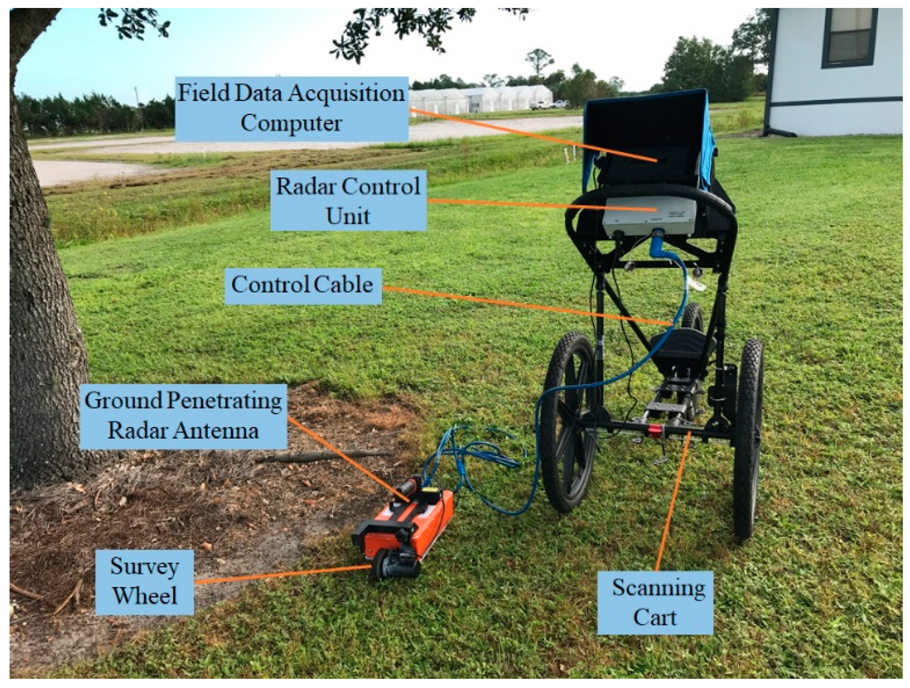
The experiments were conducted at the citrus research grove of the University of Florida Southwest Florida Research and Education Center (SWFREC) in Immokalee, FL, USA. The climate is humid subtropical, with a mean annual temperature of approximately 23 °C, and a mean annual precipitation of 1265 mm [38,39]. The site has very deep and poorly drained soils, which were formed in sandy marine sediments (Immokalee series).

2.2. Equipment

A GPR (TRU™ Model, Tree Radar, Inc., Silver Spring, MA, USA) that was mounted to a mobile scanning cart (Figure 1) and equipped with a 1600 MHz antenna was utilized to generate a 3D map of the root system. The GPR antenna transmits electromagnetic waves (pulses) and the receiver collects the reflectance when an object is detected beneath the soil surface (Figure 2). The relative distance from the starting point was measured with a wheel recorder. Commercial software TreeWin Roots and TRU Tree Radar Unit V1.2.5) was used to generate the root morphology maps. 3D images were created to present the root layout by location and depth.
The GPR principle is based on the phenomenon in which electromagnetic waves differently reflect when they interfere with materials of different dielectric constants. The GPR sends a small pulse of energy and it analyzes the strength as well as the time that is required for the reflected signal to return. The size and the distance of the detected material are calculated on the basis of the strength and time. Figure 2 presents a “scan” (series of detected reflected signals) during the detection of a tree root. The dielectric constant(s) and conductivity of the material(s) determines the strength of the reflected signal. For example, when a pulse moves from an area of sandy soil (e.g., with a dielectric constant of 4) to a fresh root (e.g., with a dielectric constant of 13.8), it produces a very strong reflection. As the antenna moves over an object, the vertical distance (time of the reflected signal to arrive at the antenna) decreases until the antenna is above the object, and it increases as the antenna moves past the object; therefore, a single object will appear in the GPR output data as a hyperbola (Figure 2). The target is located at the peak of the hyperbola (Figure 2).

2.3. Experimental Design

The roots that were removed from excavated citrus trees were used for one subset of experiments. Tree branches were used as root proxies for another subset of experiments. The roots and root proxies had diameters of 0.5 to 3 cm.

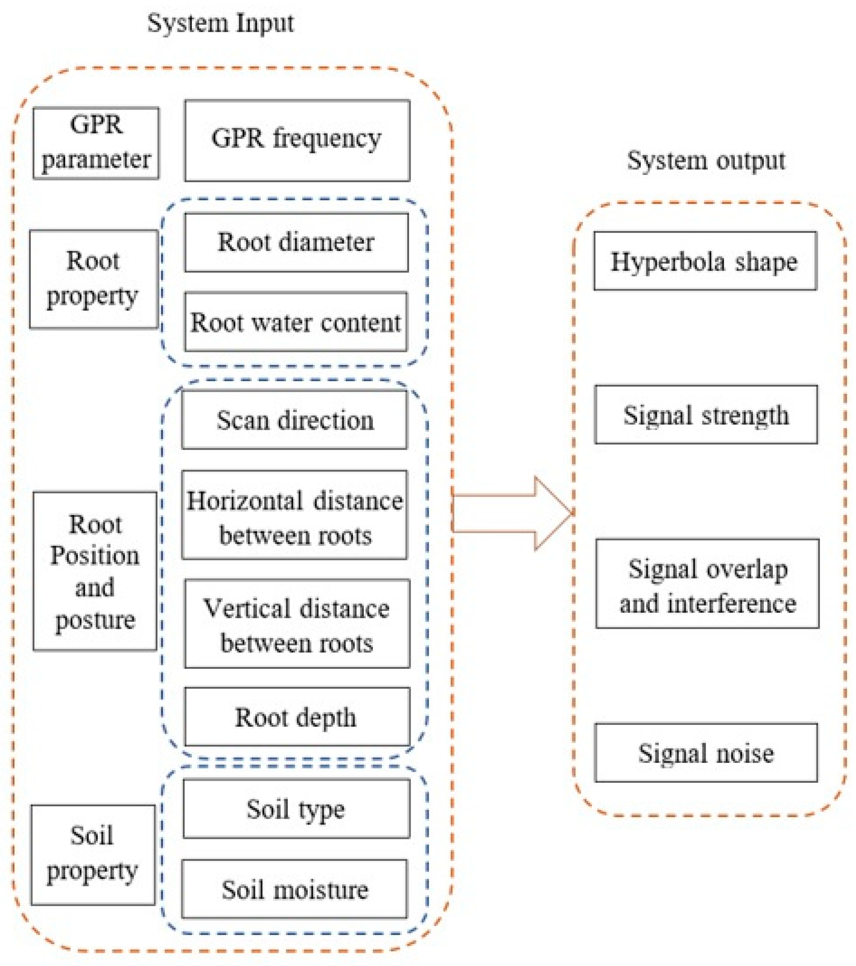
2.3.1. Experimental Factors

According to the GPR work principle, three subsystems must be investigated at the outset for accurate root detection: (I) the tree root system; (II) the soil system; and, (III) the GPR system [22] (Figure 3). In this study, three types of limiting factors were studied: (1) root properties (root diameter and root water content); (2) root position (root depth, horizontal, and vertical distance between roots) and scan direction; and, (3) soil properties (soil type and moisture). Four “output” parameters were evaluated (Figure 3): (i) the shape of the hyperbola; (ii) the signal strength; (iii) the signal overlap and interference; and, (iv) the signal noise.

2.3.2. Experiments

Different single-factor experiments (I–VII) and multi-factor experiments (VIII and IX) were conducted (Table S1). The single-factor experiments studied the effects of an individual factor on GPR performance, while controlling for all other factors. The two multi-factor experiments (validation experiments) were designed to analyze the detection accuracy of the GPR by comparing the produced maps with the actual tree root structure (by excavating the roots).

Experiments I–VII: Single-Factor Experiments

For experiments I–VII, a modified protocol that was based on the methods in references [25] and [40] was used; citrus tree branches were used as root proxies. The experimental site was scanned with the 1600 MHz GPR before experimentation to ensure that no interfering objects were present in the soil. Narrow ditches were dug instead of the holes that were described in reference [40]. In each experiment, the start line, end line, and survey lines were traced on the ground (Figure 4); the experiments were repeated three times each.
In experiment I, the effect of root diameter on the GPR detection accuracy was investigated, and eight root diameters were studied (Table S1). Live and dead root proxies were used to evaluate the effect of root water content on the GPR root detection accuracy in experiment II. The GPR detects objects through reflection; it sends electromagnetic waves and receives the reflection from the interface of two materials with different dielectric constants (e.g., soil and root). Larger differences between the dielectric constants of objects, such as between roots and soil, result in stronger reflected signals. The dielectric constant increases as the water content increases. The reflective intensity depends on the reflective coefficient, which can be obtained by calculating the relative dielectric constants of the two mediums at the interface (Equation (1)):
R = ε 1 ε 2 ε 1 + ε 2
where R is the reflection coefficient, ε 1 is the dielectric constant of medium 1, and ε 2 is the relative dielectric constant of medium 2. In this study, ε 1 and ε 2 are the relative dielectric constants of the soil and the root, respectively. In experiment II, the soil type was sandy; the average soil moisture was 6%. The dielectric constant was 4 for soil, 13.8 for fresh roots, and 5 for dead roots [39].
In experiment III, the effect of the scan angle (survey scan direction), relative to root orientation, on detection accuracy was investigated. The survey angles that were assessed were 0°, 15°, 30°, 45°, 60°, 75°, and 90° (Figure 4).
The horizontal and vertical resolutions of the GPR were evaluated for experiments IV and V. The horizontal resolution is defined as the size of the smallest target that can be horizontally detected. The horizontal resolution of a GPR depends on the first Fresnel radius (rf). When the spacing between the transmitting and receiving antennas is much smaller than the distance of the antennas from the target, the first Fresnel radius (rf) can be calculated from Equation (2) [40]:
r f = ( h + λ / 4 ) 2 h 2 = λ h / 2
where h is the depth of the target and λ is the length of the radar subwave. The GPR can only distinguish two targets when the distance between them is greater than the first Fresnel radius. The horizontal resolution decreases with the depth of an object and it depends on the wavelength of an electromagnetic wave.
In experiment IV, two root proxies were buried at the same depth (25 cm), with different distances between them (3, 5, 10, 15, and 20 cm). The minimum theoretical horizontal distance (horizontal resolution) at which roots could be detected and distinguished as separate objects at a depth of 25 cm with the 1600 MHz antennas was calculated to be 10.2 cm with Equation (2). Therefore, two roots at 25 cm depth with a lateral distance of less than 10 cm should appear as one object.
In experiment V, two root proxies were buried in the same horizontal position but at different depths (1, 3, 5, 10, and 15 cm). Five vertical distances (Table S1) between the two roots were studied to evaluate the GPR detection accuracy and the vertical resolution. The vertical resolution of a GPR depends on the ability to distinguish two signals that were emitted at different time intervals. The vertical interval is expressed by Equation (3) [40]:
Δ h = v Δ t 2 v 2 B e f f
where ∆h is the vertical resolution, ∆t is the time interval between two adjacent signals, v is the propagation speed of the electromagnetic wave in the medium, and Beff is the effective radar bandwidth. Generally, the vertical resolution of a GPR can be approximated to half the wavelength of an electromagnetic wave in the medium. The minimum theoretical vertical spacing resolution for the 1600 MHz antennas was calculated as 4 cm with Equation (3).
In experiment VI, a root proxy was buried at different depths that ranged from 10 to 70 cm (Table S1) to evaluate the accuracy of the GPR to detect roots and their locations in the ground.
In experiment VII, different soil moisture levels and their effects on the root detection accuracy were evaluated in a 1 m2 area at the SWFREC citrus grove. The HydroSense II (model CS658) with 20 cm rods was used for measuring the volumetric water content of the soil. A 25 cm deep narrow ditch was dug to bury a root proxy of 41 cm length and 23 mm diameter. The start line, end line, and survey lines were traced on the ground, and the soil was irrigated to the desired moisture level (Table S1) and monitored in 20-minute intervals. The root was scanned three times and the experiment was repeated twice on consecutive days.

Experiment VIII: Simulated Tree Root Experiment

This experiment evaluated the overall effectiveness and accuracy of the GPR for root detection. A flat area (2 × 2 m) at the SWFREC citrus grove was selected. Ten freshly harvested roots with different diameters were arranged in a pattern that simulated a tree root system (Figure 5). Roots 1–5 were buried at a flat surface parallel to the ground and at a depth of 25 cm, and roots 6–10 were buried at a slope with an angle of 15° to the ground surface, and at a depth of 25 cm (Table S2). Six circles with radii of 15, 30, 45, 60, 75, and 90 cm from the center of the arrangement were traced, and the area was scanned three times along each radius with 900 MHz GPR and 1600 MHz GPR. Table S2 lists the length and depth of each root. Table S3 presents the actual relative distances between the roots. The TreeWin Roots and the TRU Tree Radar Unit software programs were used to process data and create the 3D figures.

Experiment IX: Tree Root Field Experiment

We conducted field experiments with a five-year old Hamlin sweet orange (C. sinensis) tree on X-639 (C. reticulata × P. trifoliata) rootstock located in the SWFREC grove and affected by HLB (Figure 6) to further study and evaluate the performance of the GPR technology. The tree was 178 cm tall, with a canopy width of 205 cm and a distance of 30 cm between the soil surface and canopy base. Weeds and other objects were removed from the experimental area before the experiment, and three circles with radii of 30, 60, and 90 cm were traced. The roots were scanned three times with the 1600 MHz GPR. After the assessment, the tree was excavated, and the location and diameter of roots were measured.

2.4. Data Processing

Radar profile normalization and filtration routines were performed with the TreeWin Roots and the TRU Tree Radar Unit software programs for Windows. A background removal filter was applied to eliminate the parallel bands that were observed in the scans. The roots were detected by the GPR on the basis of a higher amplitude reflection waveform as compared with the surrounding area in the radar profiles and the appearance of a hyperbola. The positions of the roots were analyzed by combining software automatic identification with manual observations.

3. Results

3.1. Effects of Root Properties on Detection Accuracy

Experiments I and II were conducted with branches as root proxies that were buried in a narrow ditch at a depth of 25 cm. Table 1 shows the radar profiles that were measured with the 1600 MHz GPR. The shape of the hyperbola of the dead root proxy (30 mm diameter) was not well defined and its signals were weak. However, all live roots generated a well-defined hyperbola and were therefore clearly detected. From the radar profiles, the root diameters were determined by measuring the width of the hyperbolas and the strength of the signals. The hyperbolas became wider as root diameters became larger, and a greater contrast between the white and the black areas (signals) was visible; therefore, the reflected signals became stronger. The hyperbola had apparent upper and lower boundaries. The relationship between the measured diameter and the width of the hyperbola was linear (Figure 7a). The location of each root (with different diameters), which included horizontal distance and depth, was accurately assessed with an error of 1.5 cm (±2.2 cm standard deviation) for horizontal distance and an error of 0.8 cm (±1.5 cm standard deviation) for depth (Table 1). The relative error ranged from −4 to 12% (Figure 7b).

3.2. Effect of Survey Line Direction on Root Detection

In experiment III, one live root with a diameter of 29 mm was buried in a narrow ditch at the depth of 25 cm. In this experiment, the effect of the direction of the survey lines relative to the direction of the root was evaluated. The survey angles assessed were 0°, 15°, 30°, 45°, 60°, 75°, and 90°. Table 2 shows radar profiles.
The survey angle had a large influence on the shape of the hyperbola. At a survey angle of 0° to 15°, it was difficult to detect roots; with an increase in the scan angle to 30° and 45°, hyperbolas appeared but they were not well-defined or were incomplete. At a scan angle of 75°, the hyperbola appeared, but it was asymmetrical and deformed. At a scan angle of 90°, a well-defined and complete hyperbola was detected. Thus, the clearest hyperbolic reflection of the buried root was observed when the GPR survey angle was 90°, whereas it was difficult to identify the hyperbola when the angle was less than 45°.

3.3. Effect of Horizontal Distance between Roots on Detection Accuracy

The results from experiment IV demonstrated that it is difficult to distinguish two roots that were located at a horizontal distance of less than 10 cm from each other with the 1600 MHz GPR (Table 3). The hyperbolas of the two roots overlapped and created a stronger signal than that of a single root. The overlapped hyperbola widened as the distance between roots increased. The two roots were easily detected when the distance was larger than 10 cm.

3.4. Effect of Vertical Distance between Roots on Detection Accuracy

In experiment V, two roots were buried at different vertical distances from each other. The 1600 MHz GPR was used for root detection. Hyperbolas overlapped when the vertical distance of the roots was less than 5 cm, and the roots were not discernible (Table 4), but the strength of the overlapped signals was stronger than that of a single root. When the vertical distance between the two roots was greater than 5 cm, both roots could be distinguished on the basis of their individual hyperbolas. The signal of the root positioned at a shallower depth was stronger than the signal of the root that was positioned at a greater depth.

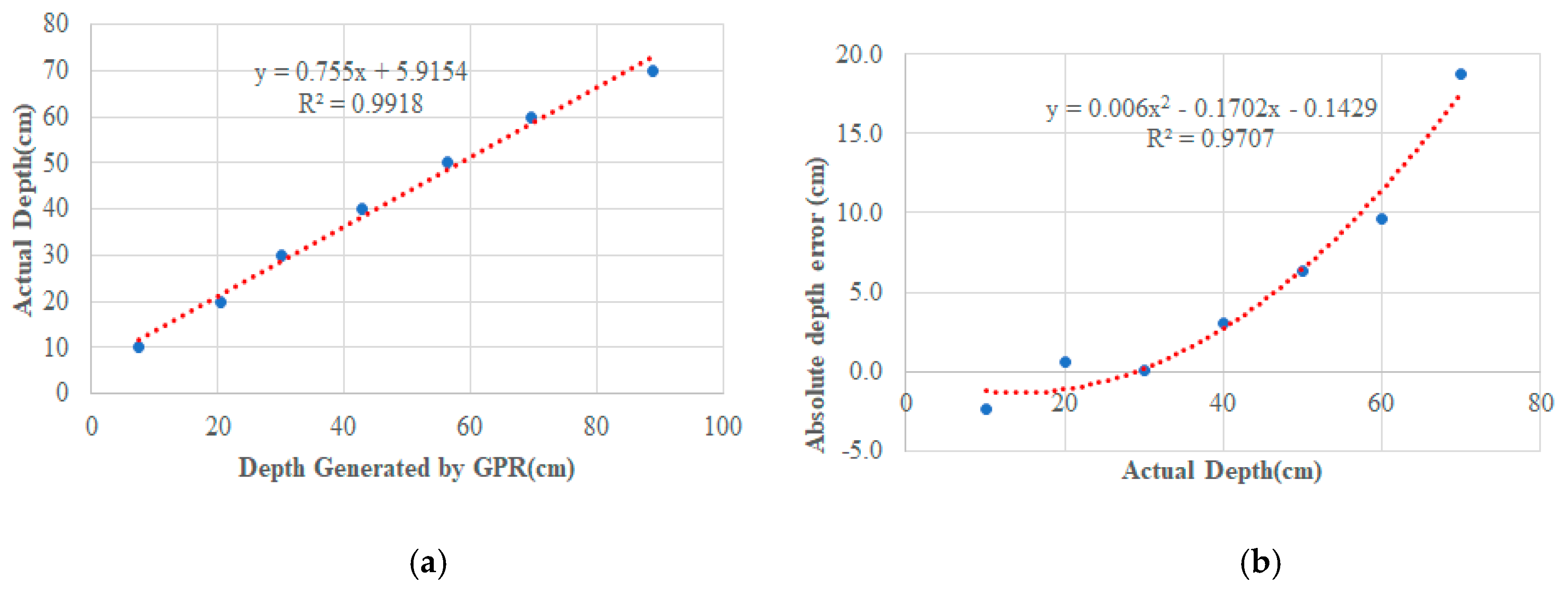
3.5. Effect of Root Depth on Root Detection Accuracy

In experiment VI, a root with a diameter of 24 mm was buried at different depths. When the depth was less than 40 cm, the upper and lower edges of the hyperbola were well-defined (Table 5). The signal began to weaken at a depth of more than 40 cm, thus resulting in the poor definition of the lower edge of the hyperbola. The reflection became even weaker at a depth of more than 60 cm, and the upper and lower edges of the hyperbola were poorly defined. The width of the hyperbola also increased with depth. The depths were measured with the radar profiles. The error of accurately determining root depth increased at increasing depths (Figure 8).

3.6. Effect of Soil Moisture on Root Detection Accuracy

Experiment VII showed that water quickly infiltrated the soil after rainfall or irrigation, and this was followed by a rapid decrease in soil moisture content from 16% to 10%. The soil moisture content remained at 10% for one hour before decreasing to 8% within the following two hours. Table 6 presents the radar profiles of root proxies buried at a depth of 25 cm and measured at different soil moisture levels. Root reflections were clear, regardless of the GPR settings and soil moisture content.

3.7. Simulated Tree Root Experiment

In experiment VIII, the live tree branches were buried as root proxies and were scanned by a 900 MHz and a 1600 MHz GPR. The TreeWin Roots and the TRU Tree Radar Unit software programs were used to create the radar profiles (Table 7). In Table 7, the vertical lines represent the actual locations of the roots (as measured in the field), and the number in the last row represents the number of the roots that are labeled before burial. The red arrow represents the detection of an actual root (true positive), the yellow arrow represents the detection of a false root (false positive), and the blue arrow represents the missed (undetected) root (false negative). Three performance metrics—accuracy, precision, and recall—were calculated (Table 8) on the basis of the signals that were generated by the GPR and described in Table 7. Precision indicates how many roots were detected correctly, and the recall measures how many roots were correctly detected.
The radar profiles that were generated by the 900 MHz GPR were less well-defined than those that were generated by the 1600 MHz GPR, thus resulting in more false positive signals (noise). The accuracy, precision, and recall averaged over the six circles was 79%, 81%, and 98% for the 900 MHz GPR and 86%, 88%, and 98% for the 1600 MHz GPR, respectively. The high recall rate indicated that our target points (roots) were accurately detected. However, other objects in the soil (e.g., stones or debris) or soil clutter can produce similar reflections and create hyperbolas, resulting in noise; therefore, lower accuracy and precision were calculated.
Figure 9 presents 3D morphology maps that were generated from TreeWin Roots and the TRU Tree Radar Unit software programs. Numbers 1–10 represent the actual buried roots (Figure 5 presents the actual locations of these roots), the black line represents the start/end line, the brown labeled lines represent the actual roots and their number, the brown non-labeled lines represent the fault roots that are created (detected) by the software, and the green dash line represents the missed root (Root #2). Both of the antennas correcly detected all roots, except root #2 (Figure 9). The 900 MHz GPR falsely detected ten more roots, in contrast to the 1600 MHz GPR, which only falsely detected four small roots. Table 9 presents the number of correcly detected roots, numbers of false positive root, accuracy, precision, and recall of the generated 3D maps. The accuracy, precision, and recall were 45%, 47%, and 90% for 900 MHz GPR and 64%, 69%, and 90% for the 1600 MHz GPR, respectively. The higher accuracy, precision, and recall of the 1600 MHz GPR than the 900 MHz indicated that the 1600 MHz GPR is more suitable for detecting citrus roots in shallow soil layers.
The angle between root #2 and the survey lines, which was less than 60° (53° in the third and about 60° in the fourth circle), may be the reason why root #2 was not detected by both of the antennas. As can be seen from Table 2, when the angle between a root and the survey line was less than 60°, the radar profile and hyperbola are not well defined. When the angle was 60°, the radar profile and hyperbola were better defined but not symmetrical. In this simulated experiment, the other nine roots were arranged in a radial direction and the survey line was nearly perpendicular to the roots, which represented the optimal situation.

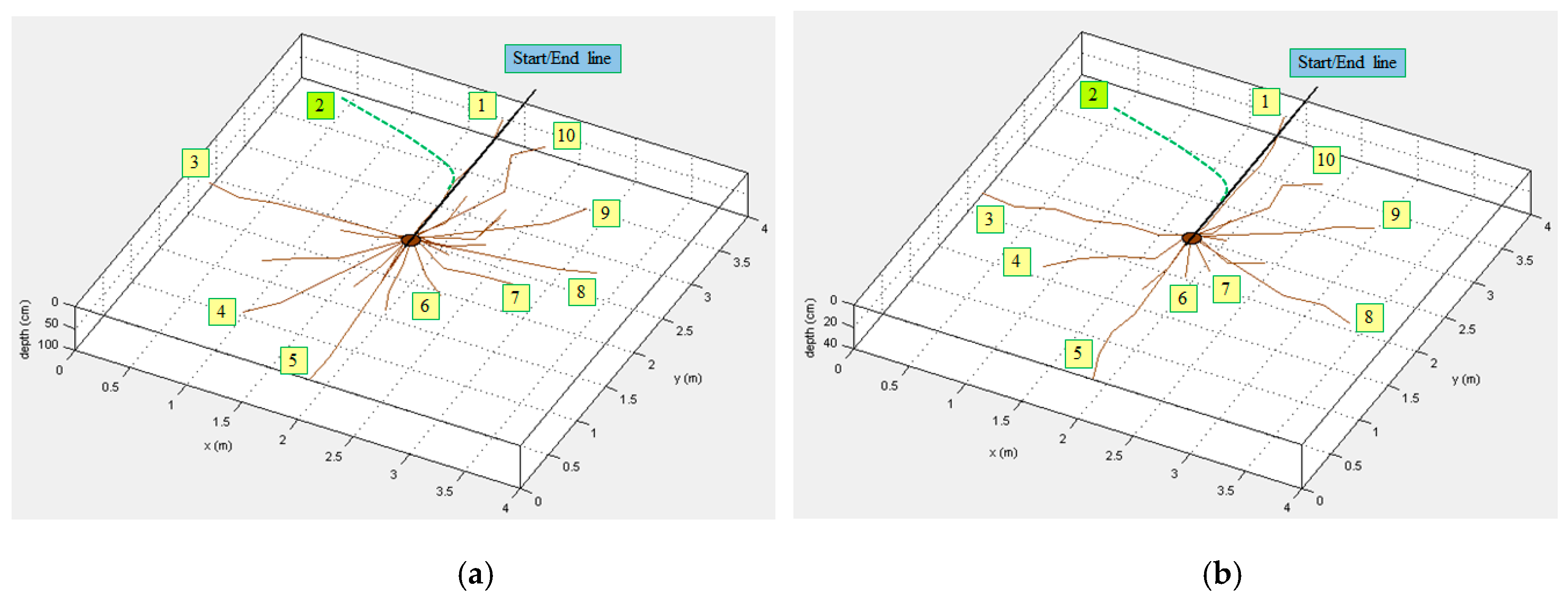
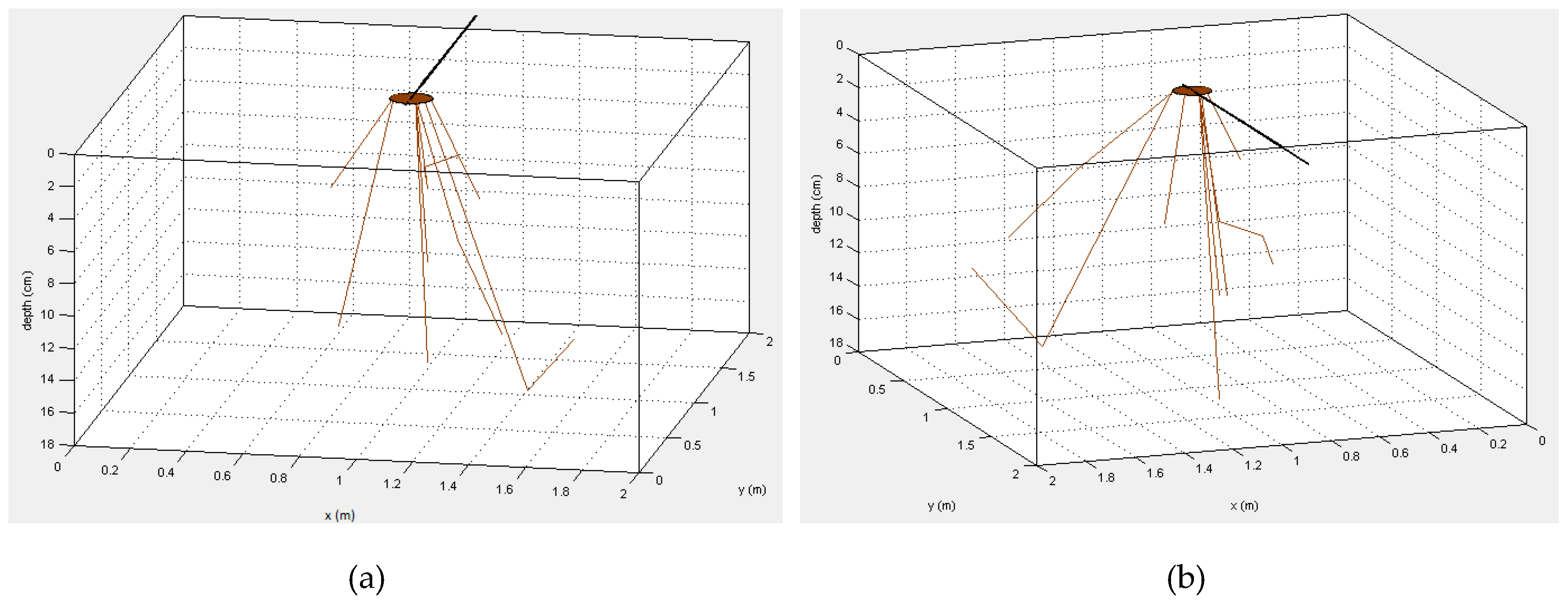
3.8. Tree Root Field Experiment with an HLB-Infected Citrus Tree

In experiment IX, the maps of the roots of an HLB-infected citrus tree were developed by using the 1600 MHz GPR (Figure 10). We measured seven long and thick roots after uprooting the tree. Most of the roots that were excavated from the site were parallel to the ground and they were located at depths of 15–25 cm. In total, we counted 46 roots, of which seven were larger than 1 cm in diameter and 39 had a diameter of less than 1 cm. In addition, numerous fibrous roots (less than 1 mm in diameter) were observed. The number and orientation of the roots that were detected by the GPR with diameter of more than 1 cm corresponded well with the actual tree root system, but roots with a diameter of less than 1 cm were not detected.
Comparison of Figure 10a,b and Figure 6b,c indicated that the 1600 MHz GPR in combination with the TreeWin Roots software program detected seven roots with a diameter lager than 1 cm with 87.5% accuracy, 87.5% precision, and 100% recall (Table 10).

4. Discussion

4.1. Effect of Water Content on Root Detection

In these experiments, the soil was sandy and the average soil moisture was 6%. The dielectric constant was 4 for the soil, 13.8 for the live roots, and 5 for the dead roots. The reflection coefficient of roots with a lower water content (representing dead roots) was less than that of roots with a higher water content (representing live roots), thus resulting in a non-well developed hyperbola of the dead roots when compared with the live roots. This method enabled the accurate determination of the water content of a root, and therefore an assessment of whether a root was alive or dead; it may be valuable for detecting the effects of diseases and new citrus management strategies on tree root architecture.
When the influence of soil moisture on GPR detection was evaluated, the results indicated that the soil water content did not affect the root reflections, thus resulting in well-defined hyperbolas. The soil dielectric constant can lower the radar’s travel speed and influence the shape of the hyperbola. As the soil dielectric constant increases, the radar wave slowly moves through the soil and the width of the hyperbola widens. The soil moisture levels at the experimental site ranged from 6% to 16%, and the corresponding relative dielectric constant was 4 to 8, which had little effect on the radar profiles.

4.2. Effect of Root Diameter on Root Detection

Root diameter affected the GPR detection accuracy and it was determined by measuring the width of the hyperbola. Previous studies have found that the accurate measurement of root diameters is difficult, especially when the diameter is less than 5 cm [41,42,43]. In our experiments, when the root diameters were less than 5 cm (but more than 0.5–1 cm), the hyperbolas had noticeable upper and lower boundaries, but it was difficult to correlate the width of the hyperbola with the diameter of the root. The signal density was higher when the tree root diameter was larger, and therefore the signal intensity was larger. Additionally, roots with a larger diameter produced brighter reflections.
Root diameter affected the relative dielectric constants of the roots. As the roots mature, they have larger root diameters, and their root porosity significantly increases. Both root diameter and root density affect the ability of the GPR to identify roots. Our results showed that the GPR with the 1600 MHz antenna detected citrus roots with diameters of more than 6 mm in sandy soil at a depth of 25 cm.

4.3. Effect of Survey Line Direction on Root Detection

Previous studies [25,26] have demonstrated that the direction of the survey line affects root detection. We recorded the highest signal intensity when the radar wave orthogonally intersected with the object. In contrast, the signal is weak if the wave front is radiated parallel to the object [28]. Under natural conditions, tree roots grow in different directions from the tree trunk center. Therefore, it would be more effective to combine circular survey lines with a grid of straight lines to improve the detection accuracy of the GPR technology. However, developing software to combine circular and straight-line measurements is very challenging.

4.4. Effect of GPR Resolution on Root Detection

The minimum theoretical horizontal distances (horizontal resolutions) at which the 1600 MHz antenna was able to distinguish roots at a depth of 25 cm was 10.2 cm (on the basis of Equation (1)). The minimum theoretical vertical spacing resolutions at which the 1600 MHz antenna could accurately detect roots was 4 cm (on the basis of Equation (2)).
The vertical resolution only depends on the wavelength of the radar and it is theoretically independent of the depth of the target. However, as the depth increases, the radar signal intensity is attenuated, so that the detection depth is limited, which thus results in a decrease in the vertical resolution. Table 5 shows that root depth affects the width of the hyperbola. With increasing the root depth, the hyperbolic width gradually increases, thus indicating that the electromagnetic wave velocity of the GPR decreases. The reflected signal intensity of roots placed at a greater depth was weaker than that of roots that were placed at a lower depth because of the weakening of the radar wave energy. Blockage of the radar signal of roots that were located deep in the soil by roots located above may also have contributed to the decreased signal intensity.
The results showed that it is difficult to detect and distinguish roots at a horizontal resolution of less than 10 cm and a vertical resolution of less than 5 cm. Further interpretation and quantitative analysis are required for overlapping or intersecting roots where the distance between roots is less than the resolution of the GPR. The 1600 MHz GPR was more suitable for the detection of shallow roots at depths less than 50 cm, and therefore provides a suitable technology for the analysis of citrus tree root systems under Florida’s growing conditions, because most of the roots are located within the upper soil horizon.

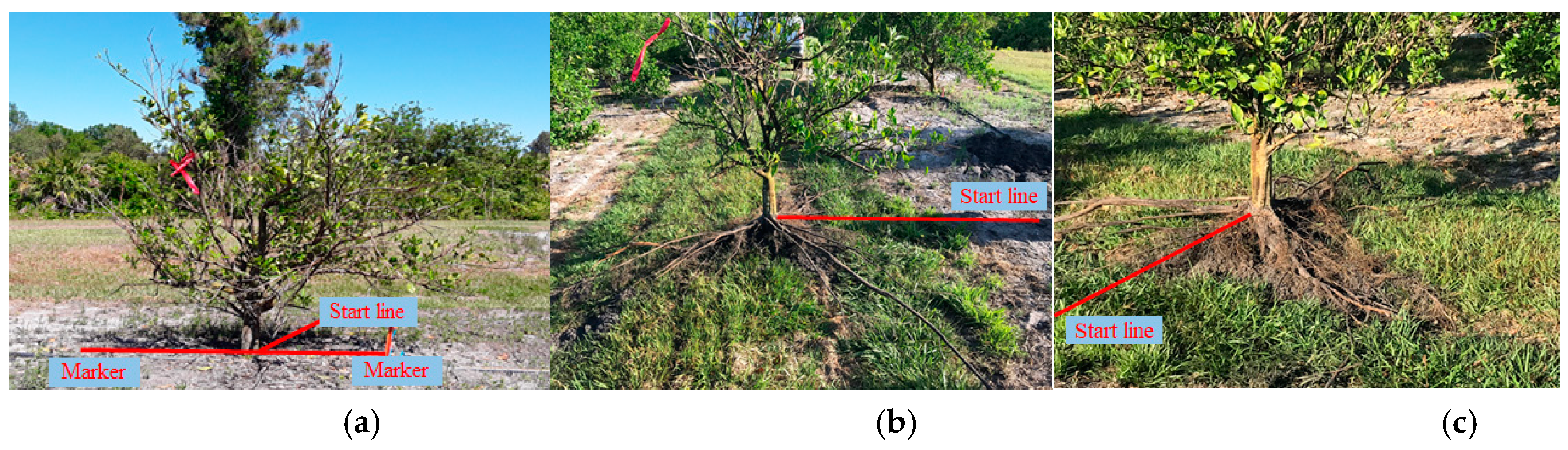
4.5. Field Tree Root Experiments

The results of the simulated tree root system experiments were consistent with the results from single-factor experiments, although some noise was detected because of irregularities in the soil environment. The angle between the location of one of the ten roots measured and the survey line was less than 60°, and the radar profile was not very clear for this root in the simulated tree root system experiment; the commercial software did not generate a root signal (root #2 in Figure 9). All other roots were mostly perpendicular to the survey line, and therefore were in the most optimal orientation for accurate detection with the 1600 MHz GPR system.
Other considerations when using a GPR for the detection of tree roots in an agricultural setting are soil moisture and soil homogeneity. Soil moisture varies depending on the rainfall and irrigation program; therefore, the GPR measurements should be scheduled in a way that minimizes these variations. In our experiments, burying root proxies resulted in mixing of different depth soils. It is recommended to assess soil horizon formation before experimentation to avoid inconsistencies in detection when using GPR for root system analysis in an agricultural setting.
Finally, it is suggested to remove all weeds around the tree trunk before collecting the data. The main challenges and limitations of the current “manual” GPR data collection procedure are: (i) maneuvering around the trees is problematic due to the lack of adequate space in the scanning area; (ii) the scanning procedure is time-consuming; (iii) often, the ground surfaces are uneven, which causes measurement errors. Hence, an automated and mobile platform for the GPR is needed to collect accurate data and reduce the operation time.

5. Conclusions

Single-factor and multi-factor field experiments were conducted to evaluate the suitability of a GPR to analyze the citrus tree root systems in an agricultural field setting. Single-factor experiments evaluated the effects of root diameter, root depth, horizontal and vertical spacing (resolution), scan detection direction, root water content, and soil moisture levels on detection accuracy. Multi-factor experiments, simulated tree root system experiments, and non-simulated (real) field experiments were designed to evaluate GPR performance and to compare the results with those of the single-factor experiments. The results demonstrated that GPR is useful for studying citrus tree root systems under southwest Florida’s growing conditions. The specific conclusions and suggestions are as follows:
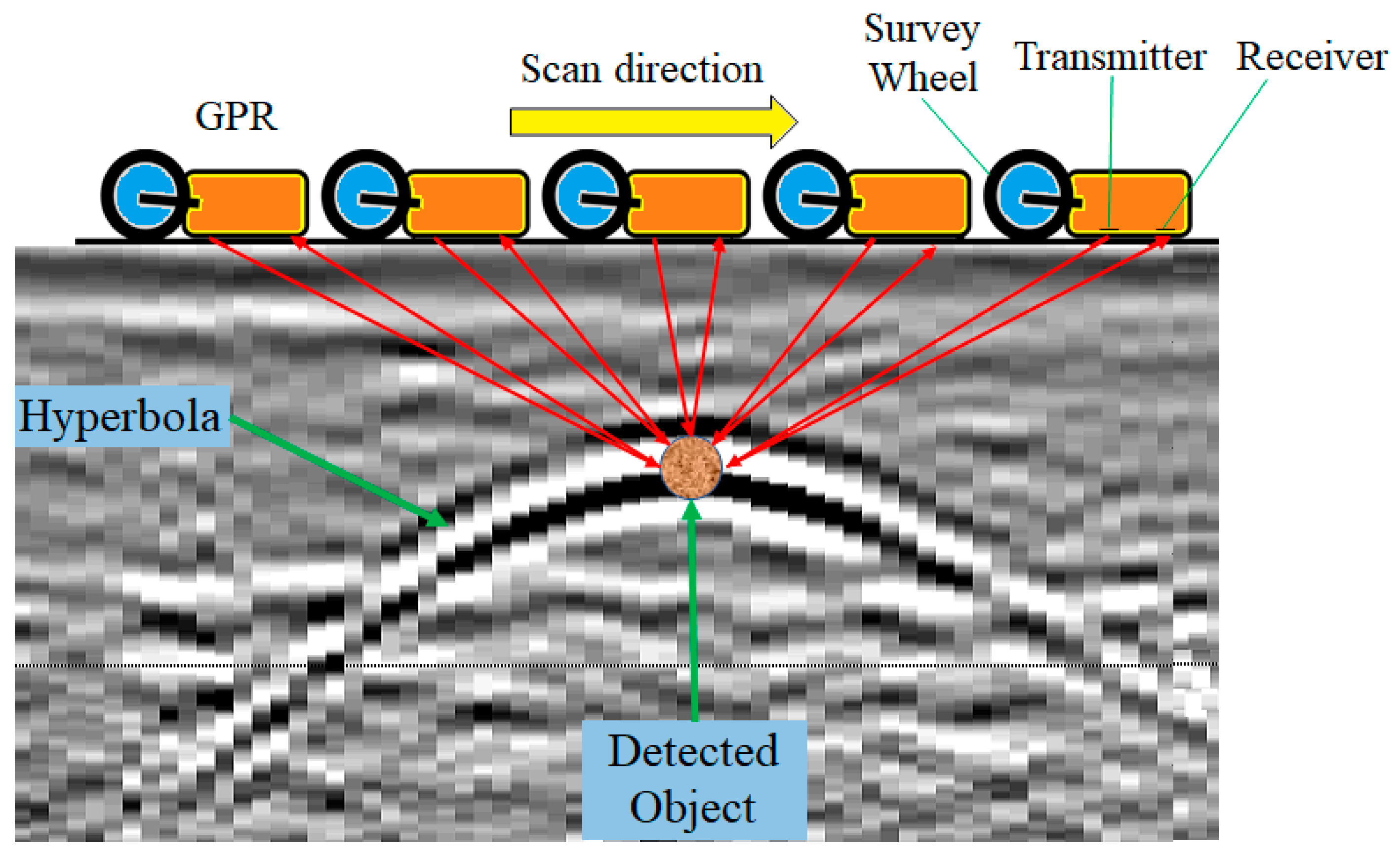
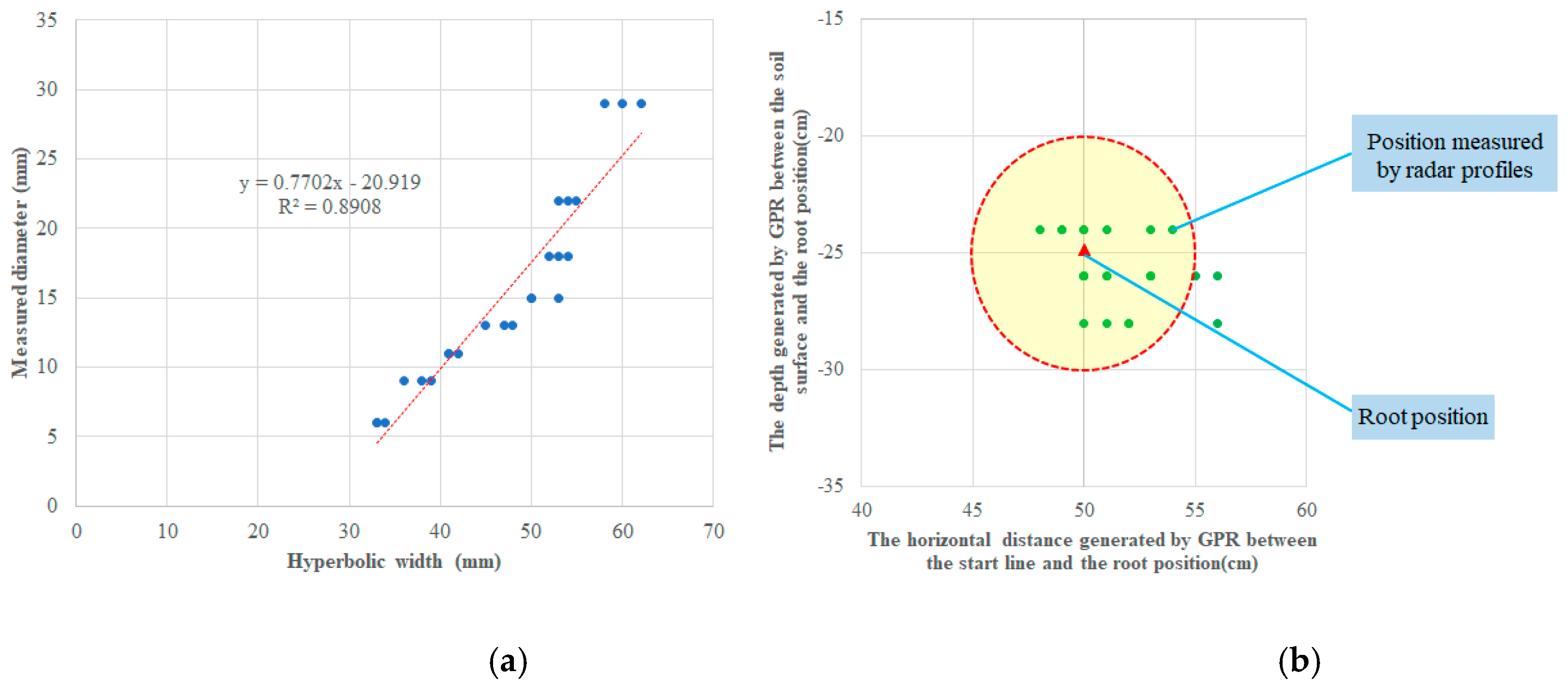
  • In a controlled environment, GPR is suitable for monitoring the roots distributed in shallow soil layers with a diameter that is larger than 6 mm. The diameter of the root influences the width of the hyperbola and the intensity (strength) of the signal. As the root diameter increases, the hyperbola widens, and consequently the reflected signal is strong. The relationship between diameter and hyperbolic widths was linear under the conditions of this study for roots with a diameter of 0.5 to 5 cm.
  • The live and dead roots were clearly distinguished in the radar profiles. The ability of the GPR system to distinguish between the live and dead roots is valuable for studying the effects of diseases, such as HLB or soil-borne pests and pathogens, on tree root growth.
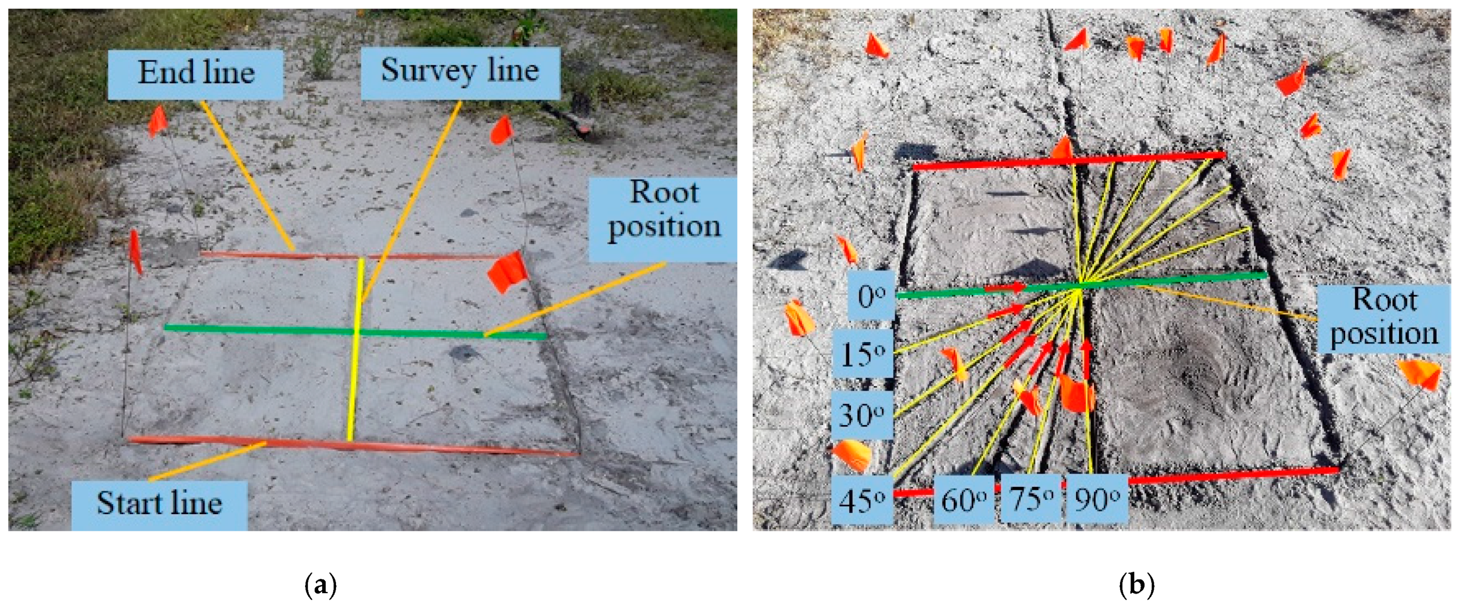
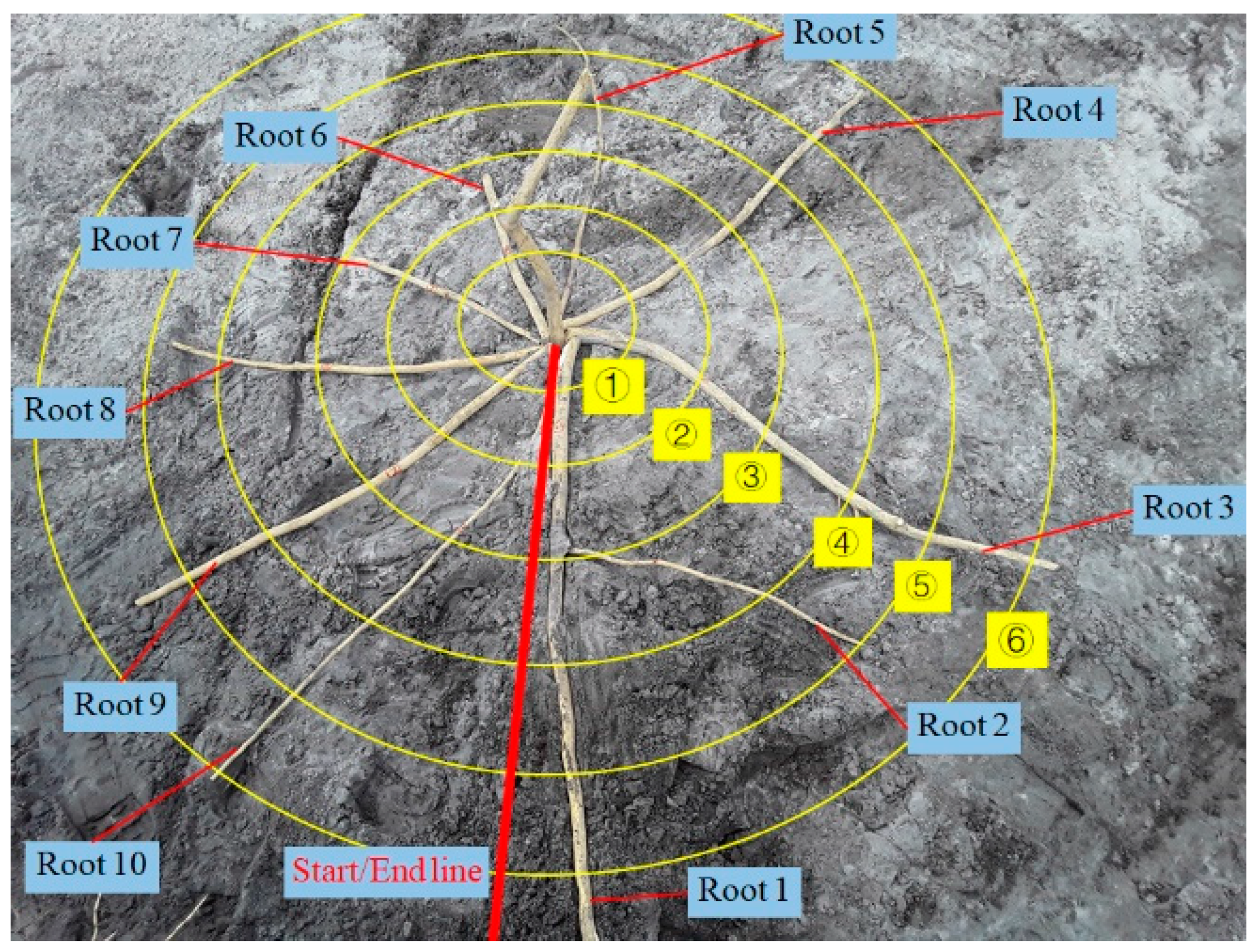
  • The direction of the survey (scan) lines strongly affects detection accuracy; keeping the survey lines perpendicular to the roots can significantly increase the GPR detection accuracy. It was difficult to identify the hyperbolas when the angle between the survey line and the direction of the root was less than 45°. Combining concentric circles with orthogonal grids would greatly improve the detection accuracy of the GPR because roots grow in various directions.
  • Two roots that were located in proximity cannot be clearly detected by 1600 MHz GPR when their horizontal distance is less than 10 cm and their vertical distance is less than 5 cm.
  • Soil water content determines the dielectric constant, which affects GPR signal generation and root detection accuracy. Sandy soil (typical of southwest Florida citrus groves) has a rapid and high water infiltration rate, which may affect GPR performance.
  • Artificial intelligence and machine learning have been utilized to correctly identify and classify objects, such as crops [44], crop pests [45,46,47], and diseases [48,49,50,51,52]. A similar approach could be adopted to automate the root detection procedure by analyzing and identify “root” hyperbolas that are produced by GPR, by utilizing artificial intelligence and machine learning.

Supplementary Materials

The following are available online at https://www.mdpi.com/2073-4395/9/7/354/s1, Table S1: Experiments and factors that were analyzed in this study, Table S2: Diameter, length, and depth of ten tree roots arranged for experiment VIII. Values were measured at six different distances (radiuses) from the center of a simulated tree root system. Radius 1 = 15 cm, radius 2 = 30 cm, radius 3 = 45 cm, radius 4 = 60, radius 5 = 75 cm, radius 6 = 90 cm, Table S3: Distance between roots arranged for experiment VIII at six different distances (radii) from the center of a simulated tree root system. Radius 1 = 15 cm, radius 2 = 30 cm, radius 3 = 45 cm, radius 4 = 60, radius 5 = 75 cm, radius 6 = 90 cm.

Author Contributions

Conceptualization, X.Z., U.A. and Y.A.; methodology, X.Z. and Y.A; validation, X.Z., M.D. and Y.A.; formal analysis, X.Z. and M.D.; investigation, X.Z., M.D. and Y.A.; resources, U.A. and Y.A.; data curation, X.Z. and M.D.; writing—original draft preparation, X.Z. and M.D.; writing—review and editing, U.A. and Y.A.; visualization, X.Z. and M.D.; supervision, U.A. and Y.A.; project administration, U.A. and Y.A.; funding acquisition, U.A. and Y.A.

Funding

This research was funded by the University of Florida Citrus Initiative and the Citrus Research and Development Foundation.

Acknowledgments

The author would like to thank Jaafar Abdulridha, Daniel Escobedo, Jorge Escobedo, Shirin Ghatrehsamani, Sri-Charan Kakarla, and Victor Henrique Meirelles-Partel for assistance with field experiments.

Conflicts of Interest

The authors declare no conflict of interest.

References

  1. Alvarez, S.; Rohrig, E.; Solis, D.; Thomas, M.H. Citrus Greening Disease (Huanglongbing) in Florida: Economic Impact, Management and the Potential for Biological Control. Agric. Res. 2016, 5, 109–118. [Google Scholar] [CrossRef]
  2. Cheng, C.Z.; Zeng, J.W.; Zhong, Y.; Yan, H.X.; Jiang, B.; Zhong, G.Y. Research progress on citrus huanglongbing disease. Acta Hortic. Sin. 2013, 40, 1656–1668. [Google Scholar]
  3. Gottwald, T.R.; da Graça, J.V.; Bassanezi, R.B. Citrus Huanglongbing: The pathogen and its impact. Plant Health Prog. 2007, 8, 31. [Google Scholar] [CrossRef]
  4. Court, C.D.; Hodges, A.W.; Rahmani, M.; Spreen, T.H. Economic Contributions of the Florida Citrus Industry in 2015–2016. Available online: https://fred.ifas.ufl.edu/pdf/economic-impact-analysis/Economic_Impacts_of_the_Florida_Citrus_Industry_2015_16.pdf (accessed on 9 May 2018).
  5. Stansly, P.A.; Arevalo, H.A.; Qureshi, J.A.; Jones, M.M.; Hendricks, K.; Roberts, P.D.; Roka, F.M. Vector control and foliar nutrition to maintain economic sustainability of bearing citrus in Florida groves affected by huanglongbing. Pest Manag. Sci. 2014, 70, 415–426. [Google Scholar] [CrossRef] [PubMed]
  6. Bowman, K.D.; Faulkner, L.; Kesinger, M. New Citrus Rootstocks Released by USDA 2001–2010: Field Performance and Nursery Characteristics. HortScience 2016, 51, 1208–1214. [Google Scholar] [CrossRef]
  7. Ghatrehsamani, S.; Abdulridha, J.; Balafoutis, A.; Zhang, X.; Ehsani, R.; Ampatzidis, Y. Development and evaluation of a mobile thermotherapy technology for in-field treatment of Huanglongbing (HLB) affected trees. Biosyst. Eng. 2019, 182, 1–15. [Google Scholar] [CrossRef] [Green Version]
  8. Jia, Z.; Ehsani, R.; Zheng, J.; Xu, L.; Zhou, H.; Ding, R. Heating characteristics and field control effect of rapid citrus huanglongbing steam heat treatment. Trans. CSAE 2017, 33, 219–225. [Google Scholar]
  9. Pertiwi, C.; Leavitt, S.; Ehsani, R.; Pelletier, W. Heat Transfer Model Development for Thermal Treatment of Huanglongbing-infected Citrus Trees. In Proceedings of the 2014 ASABE and CSBE/SCGAB Annual International Meeting, Montreal, QC, Canada, 13–16 July 2014; ASABE: St. Joseph, MI, USA, 2014. [Google Scholar]
  10. Johnson, E.; Graham, J. Roots Health in the Age of HLB. 2015. Available online: https://crec.ifas.ufl.edu/extension/trade_journals/2015/2015_August_root.pdf (accessed on 2 February 2019).
  11. Aritua, V.; Achor, D.; Gmitter, G.F.; Albrigo, G.; Wang, N. Transcriptional and Microscopic Analyses of Citrus Stem and Root Responses to Candidatus Liberibacter asiaticus Infection. PLoS ONE 2013, 8, e73742. [Google Scholar] [CrossRef]
  12. Day, S.D.; Wiseman, P.E.; Dickinson, S.B.; Harris, J.R. Contemporary Concepts of Root System Architecture of Urban Trees. Arboric. Urban For. 2010, 36, 149–159. [Google Scholar]
  13. Nadezhdina, N.; Čermák, J. Instrumental methods for studies of structure and function of root systems of large trees. J. Exp. Bot. 2003, 54, 1511–1521. [Google Scholar] [CrossRef]
  14. Judd, L.A.; Jackson, B.E.; Fonteno, W.C. Advancements in Root Growth Measurement Technologies and Observation Capabilities for Container-Grown Plants. Plants 2015, 4, 369–392. [Google Scholar] [CrossRef] [PubMed]
  15. Malamy, J. Intrinsic and environmental response pathways that regulate root system architecture. Plant Cell Environ. 2005, 28, 67–77. [Google Scholar] [CrossRef] [PubMed]
  16. Pierret, A.; Moran, C.; Doussan, C. Conventional detection methodology is limiting our ability to understand the roles and functions of fine roots. New Phytol. 2005, 166, 967–980. [Google Scholar] [CrossRef] [PubMed]
  17. Amato, M.; Basso, B.; Celano, G.; Bitella, G.; Morelli, G.; Rossi, R. In situ detection of tree root distribution and biomass by multi-electrode resistivity imaging. Tree Physiol. 2008, 28, 1441–1448. [Google Scholar] [CrossRef] [PubMed]
  18. Danjon, F.; Reubens, B. Assessing and analyzing 3D architecture of woody root systems, a review of methods and applications in tree and soil stability, resource acquisition and allocation. Plant Soil 2008, 303, 1–34. [Google Scholar] [CrossRef]
  19. Tracy, S.; Black, C.; Roberts, J.; Sturrock, C.; Mairhofer, S.; Craigon, J.; Mooney, S. Quantifying the impact of soil compaction on root system architecture in tomato (Solanum lycopersicum) by X-ray micro-computed tomography. Ann. Bot. 2012, 110, 511–519. [Google Scholar] [CrossRef] [PubMed] [Green Version]
  20. Alani, A.M.; Bianchini, C.L.; Lantini, L.; Tosti, F.; Benedetto, A. Mapping the root system of matured trees using ground penetrating radar. In Proceedings of the 17th International Conference on Ground Penetrating Radar (GPR), Rapperswil, Switzerland, 18–21 June 2018. [Google Scholar]
  21. Jol, H.M. Ground Penetrating Radar: Theory and Application; Elsevier Science: Oxford, UK, 2009. [Google Scholar]
  22. Guo, L.; Chen, J.; Cui, X.; Fan, B.; Lin, H. Application of ground penetrating radar for coarse root detection and quantification: A review. Plant Soil 2013, 362, 1–23. [Google Scholar] [CrossRef]
  23. Molon, M.; Boyce, J.; Arain, M. Quantitative, nondestructive estimates of coarse root biomass in a temperate pine forest using 3-D ground-penetrating radar (GPR). J. Geophys. Res. Biogeosci. 2017, 122, 80–102. [Google Scholar] [CrossRef]
  24. Bain, J.; Day, F.; Butnor, J. Experimental Evaluation of Several Key Factors Affecting Root Biomass Estimation by 1500 MHz Ground-Penetrating Radar. Remote Sens. 2017, 9, 1337. [Google Scholar] [CrossRef]
  25. Tanikawa, T.; Hirano, Y.; Dannoura, M.; Yamase, K.; Aono, K.; Ishii, M.; Igarashi, T.; Ikeno, H.; Kanazawa, Y. Root orientation can affect detection accuracy of ground-penetrating radar. Plant Soil 2013, 373, 317–327. [Google Scholar] [CrossRef]
  26. Tanikawa, T.; Dannoura, M.; Yamase, K.; Ikeno, H.; Hirano, Y. Reply to: “Comment on root orientation can affect detection accuracy of ground-penetrating radar”. Plant Soil 2014, 380, 445–450. [Google Scholar] [CrossRef]
  27. Guo, L.; Wu, Y.; Chen, J.; Hirano, Y.; Tanikawa, T.; Li, W.; Cui, X. Calibrating the impact of root orientation on root quantification using ground-penetrating radar. Plant Soil 2015, 395, 289–305. [Google Scholar] [CrossRef]
  28. Liu, Q.; Cui, X.; Liu, X.; Chen, J.; Chen, X.; Cao, X. Detection of Root Orientation Using Ground-Penetrating Radar. IEEE Trans. Geosci. Remote Sens. 2018, 56, 93–104. [Google Scholar] [CrossRef]
  29. Pasolli, E.; Melgani, F.; Donelli, M. Automatic Analysis of GPR Images: A Pattern-Recognition Approach. IEEE Trans. Geosci. Remote Sens. 2009, 47, 2206–2217. [Google Scholar] [CrossRef]
  30. Janning, R.; Busche, A.; Horvath, T.; Schmidt-Thieme, T. Buried pipe localization using an iterative geometric clustering on GPR data. Artif. Intell. Rev. 2014, 42, 403–425. [Google Scholar] [CrossRef]
  31. Birkenfeld, S. Automatic detection of reflexion hyperbolas in GPR data with neural networks. In Proceedings of the 2010 World Automation Congress, Kobe, Japan, 19–23 September 2010; pp. 1189–1194. [Google Scholar]
  32. Li, W.; Cui, X.; Guo, L.; Chen, J.; Chen, X.; Cao, X. Tree Root Automatic Recognition in Ground Penetrating Radar Profiles Based on Randomized Hough Transform. Remote Sens. 2016, 8, 430. [Google Scholar] [CrossRef]
  33. Freeland, R.S. Imaging the lateral roots of the orange tree using three-dimensional GPR. J. Environ. Eng. Geophys. 2015, 20, 235–244. [Google Scholar] [CrossRef]
  34. Freeland, R.S. Surveying the Near-Surface Fibrous Citrus Root System of the Orange Tree With 3-D GPR. Appl. Eng. Agric. 2016, 32, 145–153. [Google Scholar]
  35. Tan, P.Y.; Jim, C.Y. Greening Cities: Forms and Functions; Springer: Singapore, 2017; p. 295. [Google Scholar]
  36. Peterson, C.; Soares, T.; Torbert, E.; Herrera, I.; Scow, K.; Gaudin, A.C.M. Drip Irrigation Effect on Soil Function, Root Systems and Productivity in Organic Tomato and Corn. In Proceedings of the Organic Agriculture Research Symposium, Pacific Grove, CA, USA, 20 January 2016; pp. 1–7. [Google Scholar]
  37. Morgan, K.T.; Obreza, T.A.; Scholberg, J.M.S. Orange tree fibrous root length distribution in space and time. J. Am. Soc. Hortic. Sci. 2007, 132, 262–269. [Google Scholar] [CrossRef]
  38. United States Climate Data—Version 2.3—Programming and Design by Your Weather Service-World Climate-Weernetwerk. 2018. Available online: https://www.usclimatedata.com/climate/immokalee/florida/united-states/usfl0216 (accessed on 5 February 2019).
  39. United States of Agriculture—Natural Resources Conservation Service—Official Soil Series Descriptions. 2018. Available online: https://soilseries.sc.egov.usda.gov/OSD_Docs/I/IMMOKALEE.html/ (accessed on 5 February 2019).
  40. Guo, L.; Cui, X.; Chen, J. Sensitive factors analysis in using GPR for detecting plant roots based on forward modeling. Prog. Geophys 2012, 27, 1745–1763. [Google Scholar]
  41. Barton, C.; Montagu, K. Detection of tree roots and determination of root diameters by ground penetrating radar under optimal conditions. Tree Physiol. 2004, 24, 1323–1331. [Google Scholar] [CrossRef] [PubMed] [Green Version]
  42. Cui, X.; Chen, J.; Shen, J.; Cao, X.; Chen, X.; Zhu, X. Modeling tree root diameter and biomass by ground-penetrating radar. Sci. China-Earth Sci. 2011, 54, 711–719. [Google Scholar] [CrossRef]
  43. Mucciardi, T. Tree Radar (Radar Imaging for Non-Invasive Assessment of Tree and Root Health). 2004. Available online: http://treeradar.com/TRUSystem.htm (accessed on 5 January 2019).
  44. Ampatzidis, Y.; Partel, V. UAV-based High Throughput Phenotyping in Citrus Utilizing Multispectral Imaging and Artificial Intelligence. Remote Sens. 2019, 11, 410. [Google Scholar] [CrossRef]
  45. Partel, V.; Kakarla, S.C.; Ampatzidis, Y. Development and Evaluation of a Low-Cost and Smart Technology for Precision Weed Management Utilizing Artificial Intelligence. Comput. Electron. Agric. 2019, 157, 339–350. [Google Scholar] [CrossRef]
  46. Partel, V.; Nunes, L.; Stansley, P.; Ampatzidis, Y. Automated Vision-based System for Monitoring Asian Citrus Psyllid in Orchards Utilizing Artificial Intelligence. Comput. Electron. Agric. 2019, 162, 328–336. [Google Scholar] [CrossRef]
  47. Luvisi, A.; Ampatzidis, Y.; De Bellis, L. Plant pathology and information technology: Opportunity and uncertainty in pest management. Sustainability 2016, 8, 831. [Google Scholar] [CrossRef]
  48. Abdulridha, J.; Ampatzidis, Y.; Ehsani, R.; de Castro, A. Evaluating the Performance of Spectral Features and Multivariate Analysis Tools to Detect Laurel Wilt Disease and Nutritional Deficiency in Avocado. Comput. Electron. Agric. 2018, 155, 203–2011. [Google Scholar] [CrossRef]
  49. Abdulridha, J.; Ehsani, R.; Abd-Elrahman, A.; Ampatzidis, Y. A Remote Sensing technique for detecting laurel wilt disease in avocado in presence of other biotic and abiotic stresses. Comput. Electron. Agric. 2019, 156, 549–557. [Google Scholar] [CrossRef]
  50. Cruz, A.C.; Luvisi, A.; De Bellis, L.; Ampatzidis, Y. X-FIDO: An Effective Application for Detecting Olive Quick Decline Syndrome with Novel Deep Learning Methods. Front. Plant Sci. 2017, 8, 1741. [Google Scholar] [CrossRef]
  51. Cruz, A.; Ampatzidis, Y.; Pierro, R.; Materazzi, A.; Panattoni, A.; De Bellis, L.; Luvisi, A. Detection of Grapevine Yellows Symptoms in Vitis vinifera L. with Artificial Intelligence. Comput. Electron. Agric. 2019, 157, 63–76. [Google Scholar] [CrossRef]
  52. Abdulridha, J.; Batuman, O.; Ampatzidis, Y. UAV-based Remote Sensing Technique to Detect Citrus Canker Disease Utilizing Hyperspectral Imaging and Machine Learning. Remote Sens. 2019, 11, 1373. [Google Scholar] [CrossRef]
Figure 1. A ground-penetrating radar (GPR) mounted to a scanning cart.
Agronomy 09 00354 g001
Figure 2. A GPR generates a hyperbola when an object is detected.
Agronomy 09 00354 g002
Figure 3. Input factors and output parameters of the experimental design.
Agronomy 09 00354 g003
Figure 4. Single-factor root detection experiments: (a) Start line, end line and survey line; (b) Survey line direction experiment.
Agronomy 09 00354 g004
Figure 5. Simulated tree root experiment. This figure presents the root distribution, root location, root number, and the “scan” lines (circles).
Agronomy 09 00354 g005
Figure 6. Hamlin/X-639 tree and its root system: (a) Front view of tree; (b) Front view of tree roots; and, (c) Back view of tree roots.
Agronomy 09 00354 g006
Figure 7. Evaluation of root diameter and root position. (a) Relationship between measured root diameter and width of the hyperbola. (b) Root locations measured by the GPR (the actual root position is indicated by the red triangle).
Agronomy 09 00354 g007
Figure 8. Evaluation of root depth: (a) Relationship between the actual depth and the depth measured from the GPR profiles. (b) Error of detection with increasing depth.
Agronomy 09 00354 g008
Figure 9. Three-dimensional (3D) root morphology maps generated by: (a) 900 MHz; and, (b) 1600 MHz GPR (experiment VIII). The black line represents the start/end line; the brown labeled lines represent the actual roots and their number; the brown non-labeled lines represent the fault roots created by the software; and, the green dash line represents the missed root (Root #2).
Agronomy 09 00354 g009
Figure 10. Tree root field experiment X: (a) Front view of the 3D root morphology map. (b) Back view of the 3D root morphology map. The black line represents the start/end line; the brown lines represent the roots created by the TreeWin Roots software program; and, the pink lines represent markers in the field to calibrate distances during data collection.
Agronomy 09 00354 g010
Table 1. Radar profiles of roots with different diameters and water content.
Root No.Live or DeadDiameter
(mm)
Radar
Profile
Width of Hyperbola
(mm)
Actual Distance
(cm)
Distance Generated by GPR (cm)Relative Error of Distance (%)Actual Depth
(cm)
Depth Generated by GPR (cm)Relative Error of Depth (%)
Root
1
Live6 Agronomy 09 00354 i00133505612−25−2812
33505510−25−264
34505612−25−264
Root
2
Live9 Agronomy 09 00354 i0023850536−25−264
3950536−25−264
3650548−25−24−4
Root
3
Live11 Agronomy 09 00354 i0034150500−25−264
4250500−25−264
4150500−25−2812
Root
4
Live13 Agronomy 09 00354 i0044750500−25−264
485048−4−25−24−4
4550500−25−264
Root
5
Live15 Agronomy 09 00354 i0055350500−25−24−4
5050536−25−24−4
5050512−25−24−4
Root
6
Live18 Agronomy 09 00354 i0065350524−25−2812
5450524−25−2812
5250512−25−264
Root
7
Live22 Agronomy 09 00354 i0075550512−25−2812
5450536−25−264
5350512−25−264
Root
8
Live29 Agronomy 09 00354 i0085850500−25−24−4
625049−2−25−24−4
605049−2−25−24−4
Root
9
Dead30 Agronomy 09 00354 i009 50- −25
Mean value51.5 −25.8
Standard deviation2.2 1.5
Table 2. Radar profiles of different survey line directions.
Scan Angle15°30°45°60°75°90°
Radar profile Agronomy 09 00354 i010 Agronomy 09 00354 i011 Agronomy 09 00354 i012 Agronomy 09 00354 i013 Agronomy 09 00354 i014 Agronomy 09 00354 i015 Agronomy 09 00354 i016
Detection effectNo hyperbolaNo hyperbolaNot well-defined hyperbolaNot well-defined hyperbolaIncomplete hyperbolaIncomplete hyperbolaWell-defined hyperbola
Table 3. Radar profiles of two roots buried at different horizontal distances from one another.
Actual Horizontal Distance 3 cm5 cm10 cm15 cm20 cm
Radar profile Agronomy 09 00354 i017 Agronomy 09 00354 i018 Agronomy 09 00354 i019 Agronomy 09 00354 i020 Agronomy 09 00354 i021
Detection effect1 root detected1 root detected2 roots detected2 roots detected2 roots detected
Table 4. Radar profiles of roots buried at different vertical distances from one another.
Actual Vertical Distance 1 cm3 cm5 cm10 cm15 cm
Radar profile Agronomy 09 00354 i022 Agronomy 09 00354 i023 Agronomy 09 00354 i024 Agronomy 09 00354 i025 Agronomy 09 00354 i026
Detection effect1 root detected1 root detected2 roots detected2 roots detected2 roots detected
Table 5. Radar profiles of a root buried at different depths.
Actual Depth10 cm20 cm30 cm40 cm50 cm60 cm70 cm
Radar profile Agronomy 09 00354 i027 Agronomy 09 00354 i028 Agronomy 09 00354 i029 Agronomy 09 00354 i030 Agronomy 09 00354 i031 Agronomy 09 00354 i032 Agronomy 09 00354 i033
Effect on hyperbola detectionUpper and lower edges well-definedUpper and lower edges well-definedUpper and lower edges well-definedLower edge
not well-defined
Lower edge
not well-defined
Upper and lower edges not well-definedUpper and lower edges not well-defined
Detected distance8 cm20 cm30 cm43 cm56 cm70 cm89 cm
Table 6. Radar profiles of root proxies at different soil moisture levels. GPR settings were adjusted on the basis of soil type and dielectric constant.
Actual Soil Moisture (%)Radar Profile Using Different Soil Type and Dielectric Constant
Soil Moisture Content 20%Soil Moisture Content 13%Soil Moisture Content 9%
16 Agronomy 09 00354 i034 Agronomy 09 00354 i035 Agronomy 09 00354 i036
11 Agronomy 09 00354 i037 Agronomy 09 00354 i038 Agronomy 09 00354 i039
6 Agronomy 09 00354 i040 Agronomy 09 00354 i041 Agronomy 09 00354 i042
Table 7. Radar profiles of the simulated tree root experiment.
Survey CirclesRadar profile
900 MHz1600 MHz
Circle 1 Agronomy 09 00354 i043
Circle 2
Circle 3
Circle 4
Circle 5
Circle 6
Root NO. 10 9 8 7 6 5 4 3 2 1 10 9 8 7 6 5 4 3 2 1
The red arrow represents the detection of an actual root (true positive). The yellow arrow represents the detection of a false root (false positive). The blue arrow represents the missed (undetcted) root (false negative).
Table 8. Detection accuracy, precision, and recall of the simulated experiment.
900 MHz
Survey circlesTOTPFNFPAccuracyPrecisionRecall
Circle 1990375%75%100%
Circle 2990282%82%100%
Circle 3871270%78%88%
Circle 4880189%89%100%
Circle 5880189%89%100%
Circle 6330260%60%100%
SUM454411179%81%98%
1600 MHz
Survey circlesTOTPFNFPAccuracyPrecisionRecall
Circle 1990282%82%100%
Circle 2990190%90%100%
Circle 3871178%88%88%
Circle 4880189%89%100%
Circle 5880189%89%100%
Circle 63300100%100%100%
SUM45441686%88%98%
TO, number of total actual points; TP, number of target points detected (true positives); FN, number of target points missed (false negatives); FP, number of non-targets points detected (false positives). Accuracy was calculated as TP/(TP+FP+FN); precision was calculated as TP/(TP+FP); recall was calculated as TP/(TP+FN).
Table 9. Accuracy, precision, and recall of the generated 3D maps for experiment IX.
FrequencyRTORTPRFNRFPAccuracyPrecisionRecall
900 MHz10911045%47%90%
1600 MHz1091464%69%90%
RTO, number of total actual roots; RTP, number of target roots created (true positive); RFN, number of target roots missed (false negative); RFP, number of non-target roots created (false positive). Accuracy was calculated as RTP/(RTP+ RFP+ RFN); precision was calculated as RTP/(RTP+ RFP); and recall was calculated as RTP/(RTP+ RFN).
Table 10. Accuracy, precision, and recall of experiment X for roots more than 1 cm in diameter.
FrequencyRRTORRTPRRFNRRFPAccuracyPrecisionRecall
1600 MHz770187.5%87.5%100%
RRTO, number of total actual roots (> 1 cm); RRTP, number of target roots created (> 1 cm) (true positive); RRFN, number of target roots missed (> 1 cm) (false negative); RRFP, number of non-target roots created (false positive); accuracy was calculated as RRTP/(RRTP+ RRFP+ RRFN); precision was calculated as RRTP/(RRTP+ RRFP); and recall was calculated as RRTP/(RRTP+ RRFN).

