A Case-Based Economic Assessment of Robotics Employment in Precision Arable Farming

 ,
,  ,
, 
 ,
,  ,
, 

Abstract
:1. Introduction
2. Materials and Methods
2.1. Field Efficiency of Agricultural Machinery
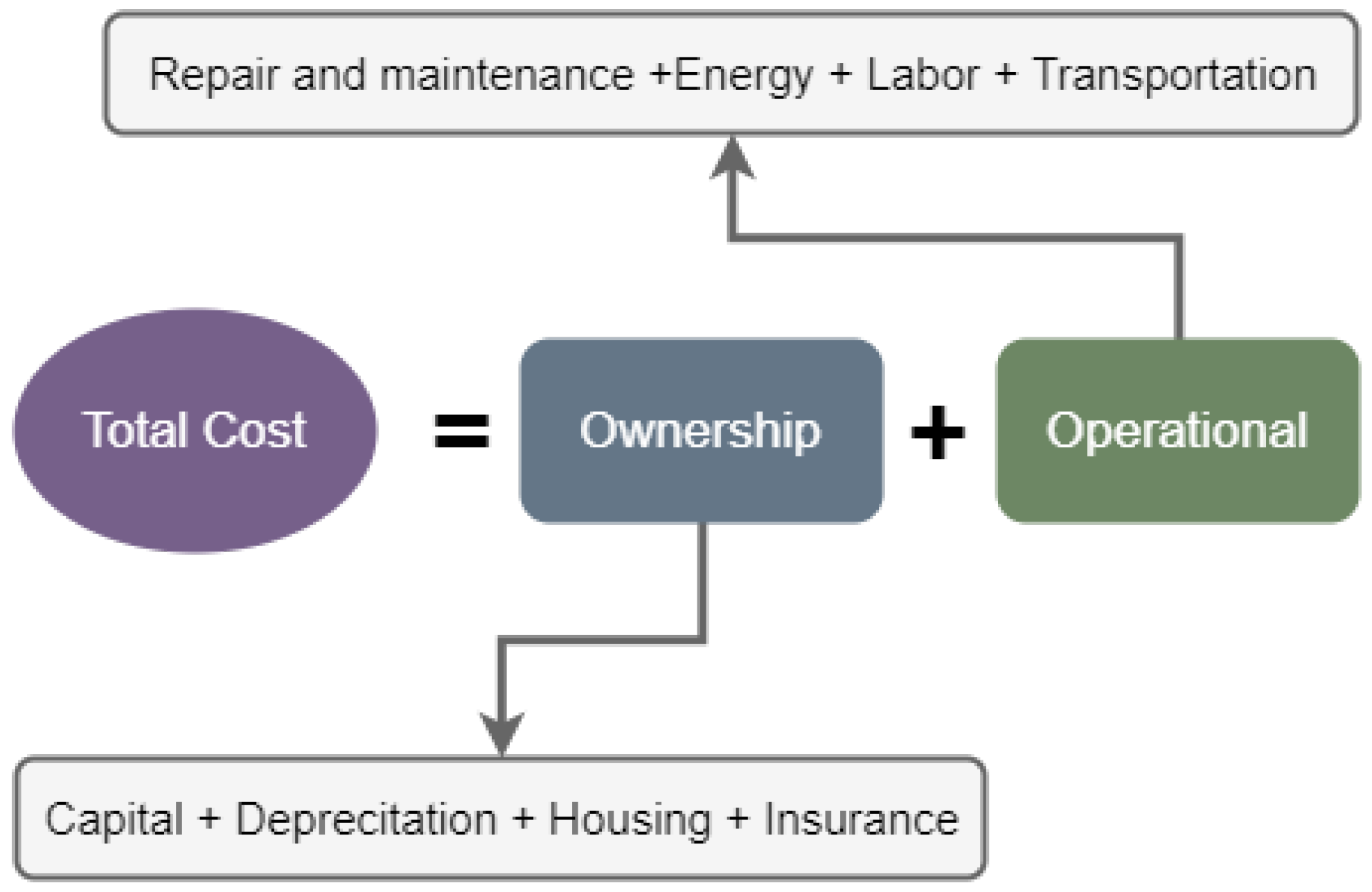
2.2. Costs Estimation Model
2.3. Case Study Description
3. Results and Discussion
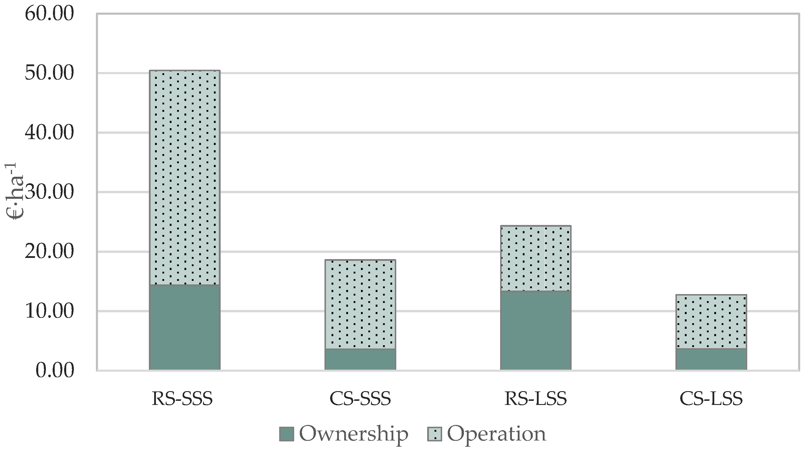
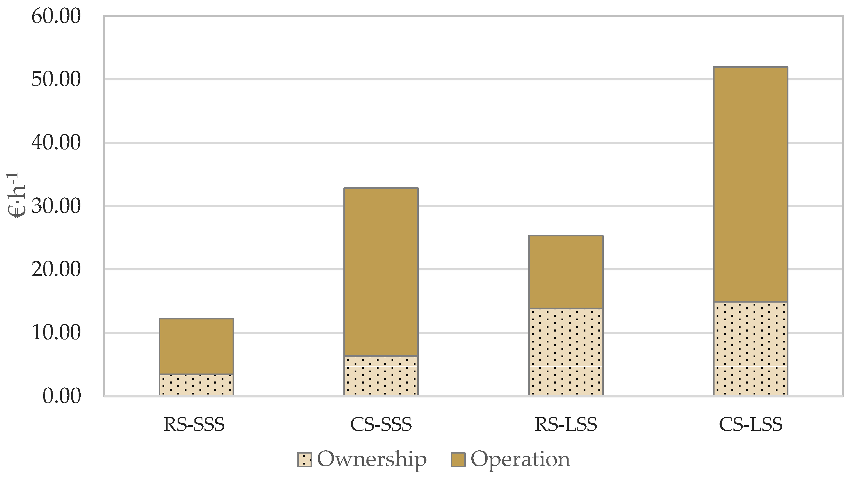
3.1. Total Cost
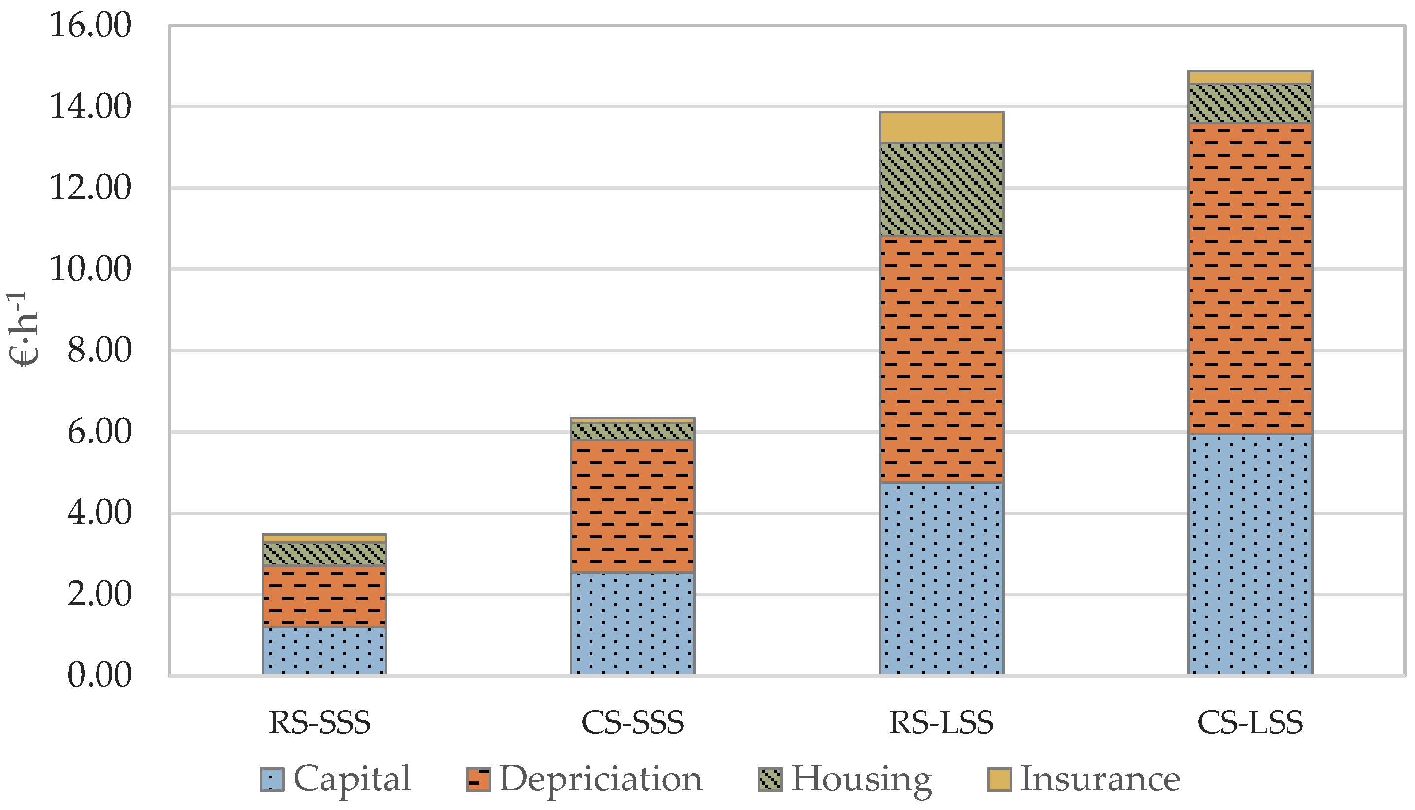
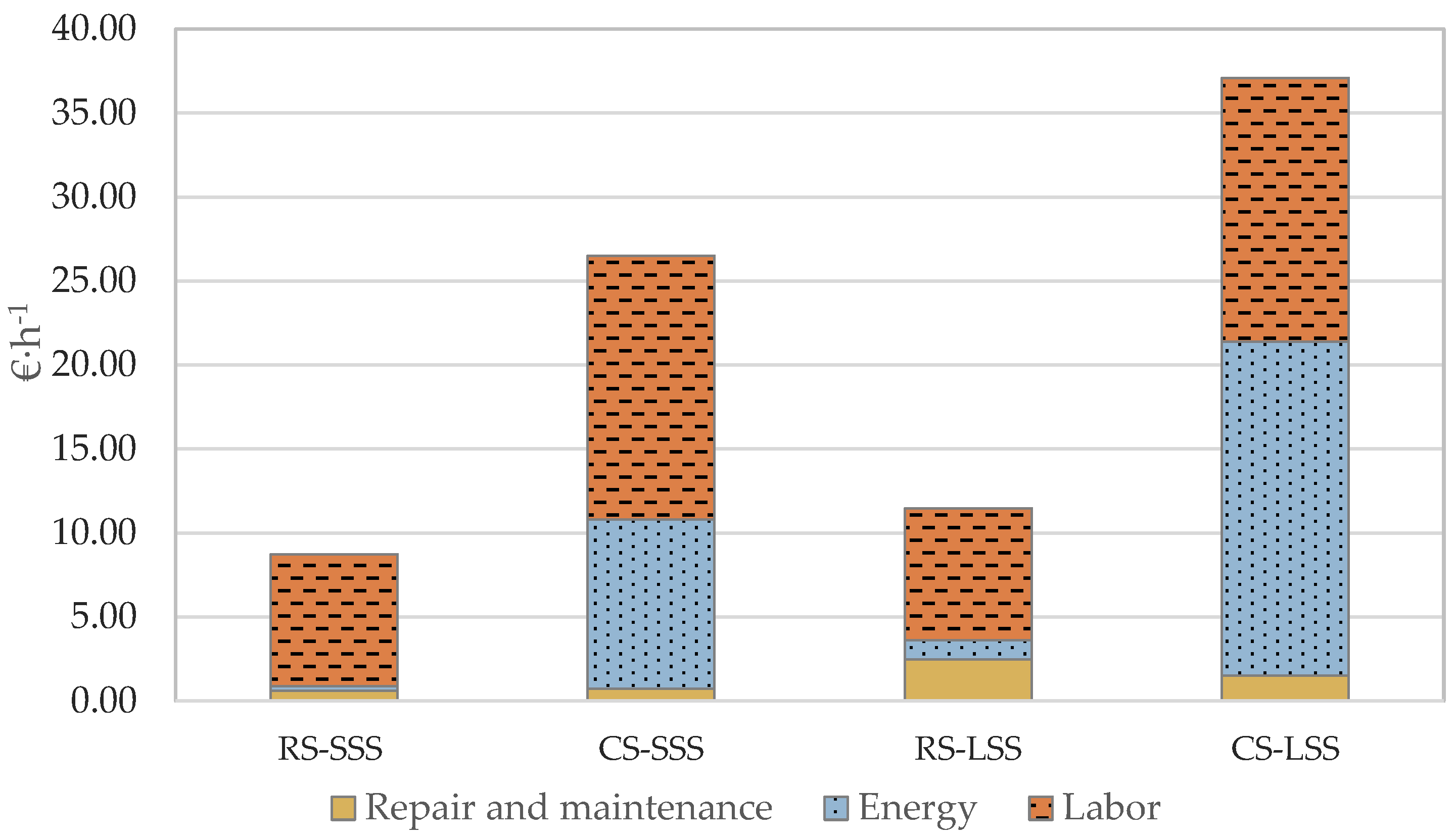
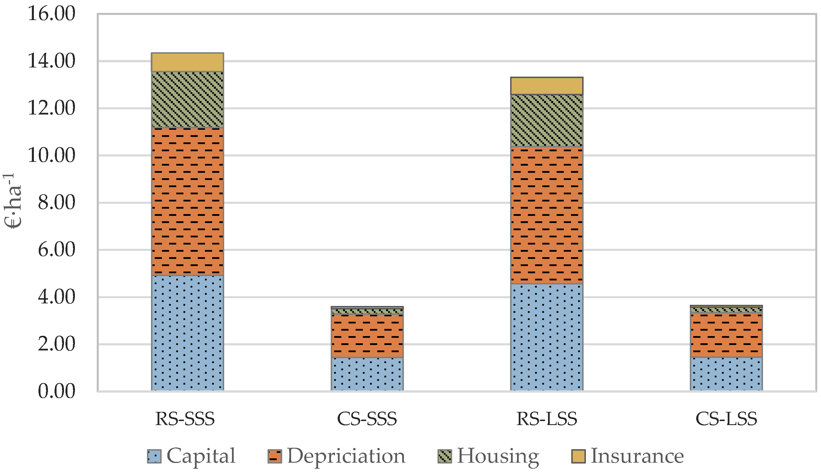
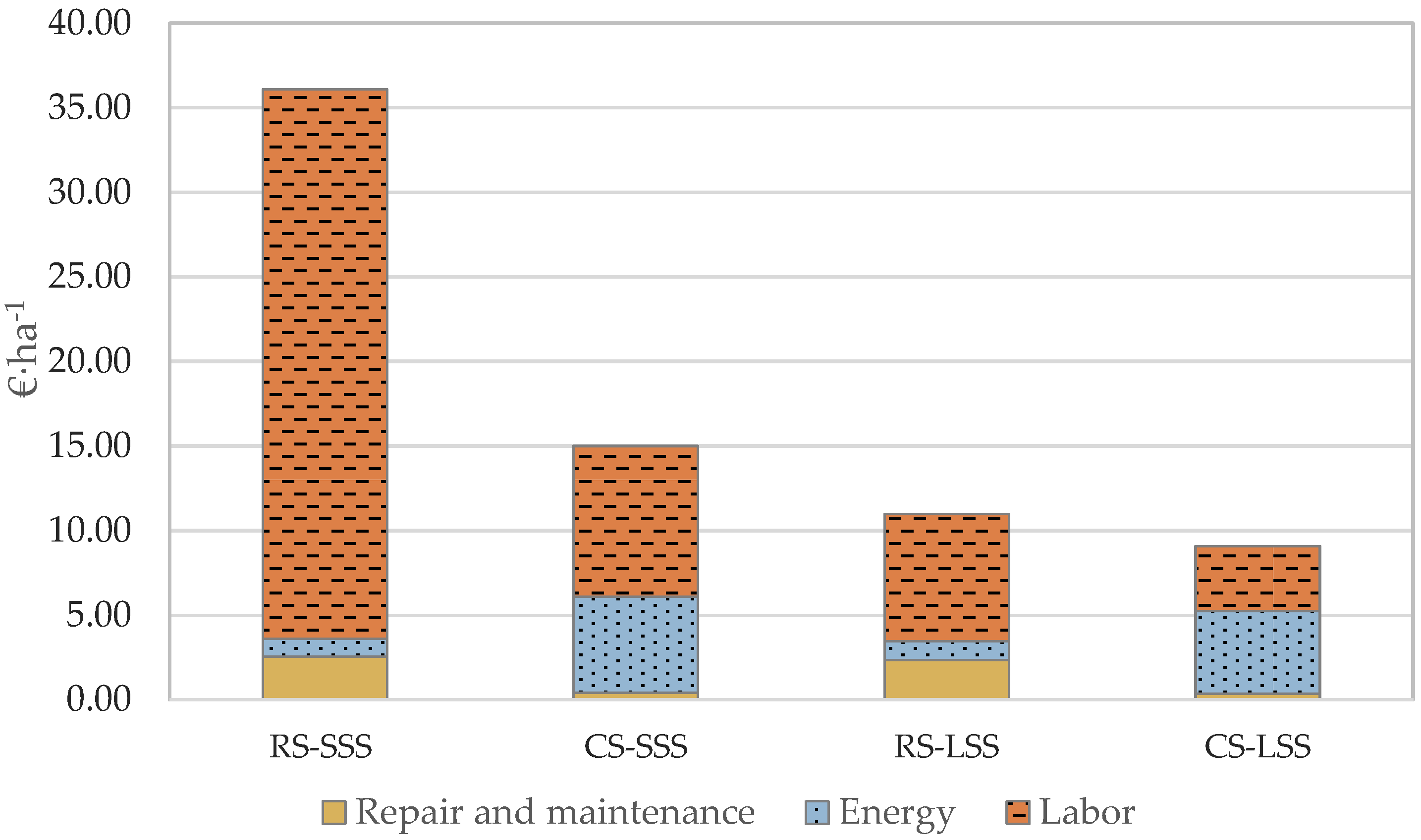
3.2. Cost Analysis
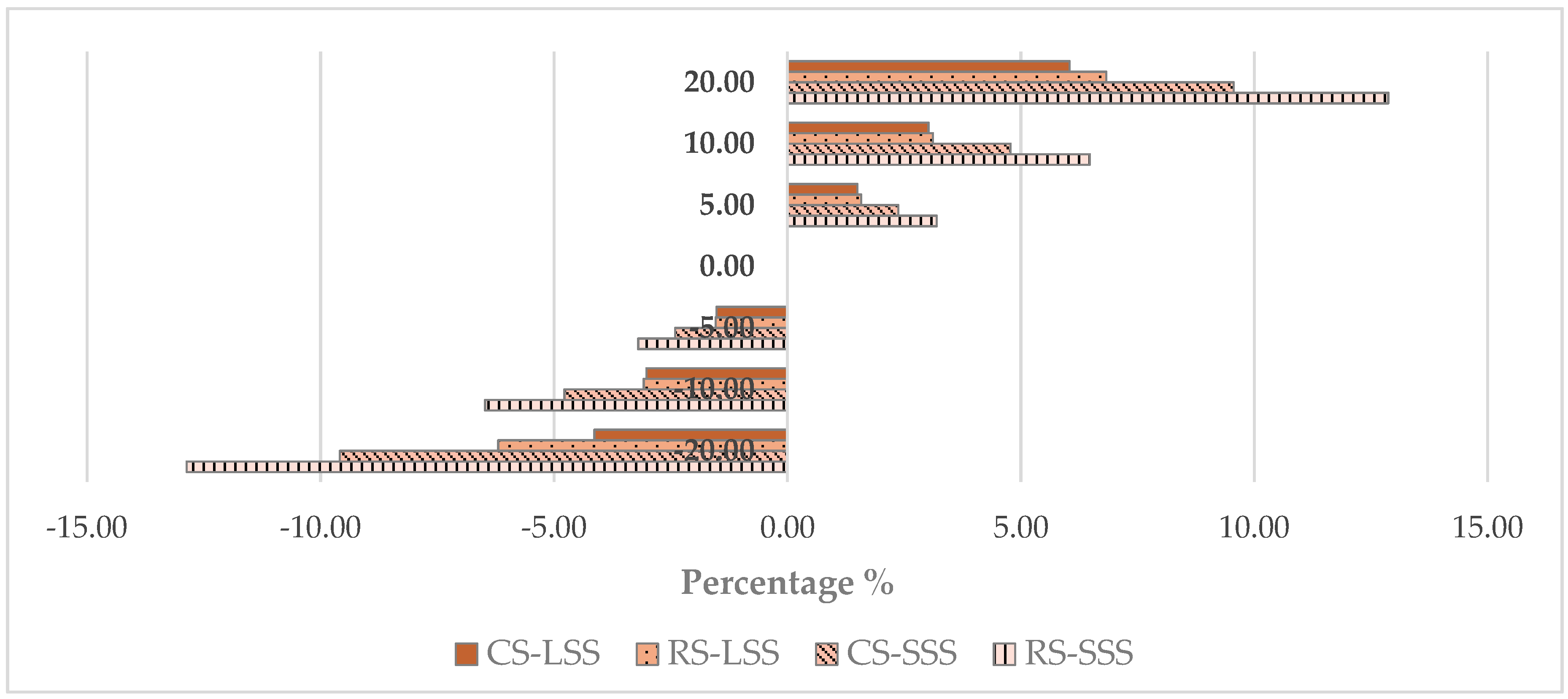
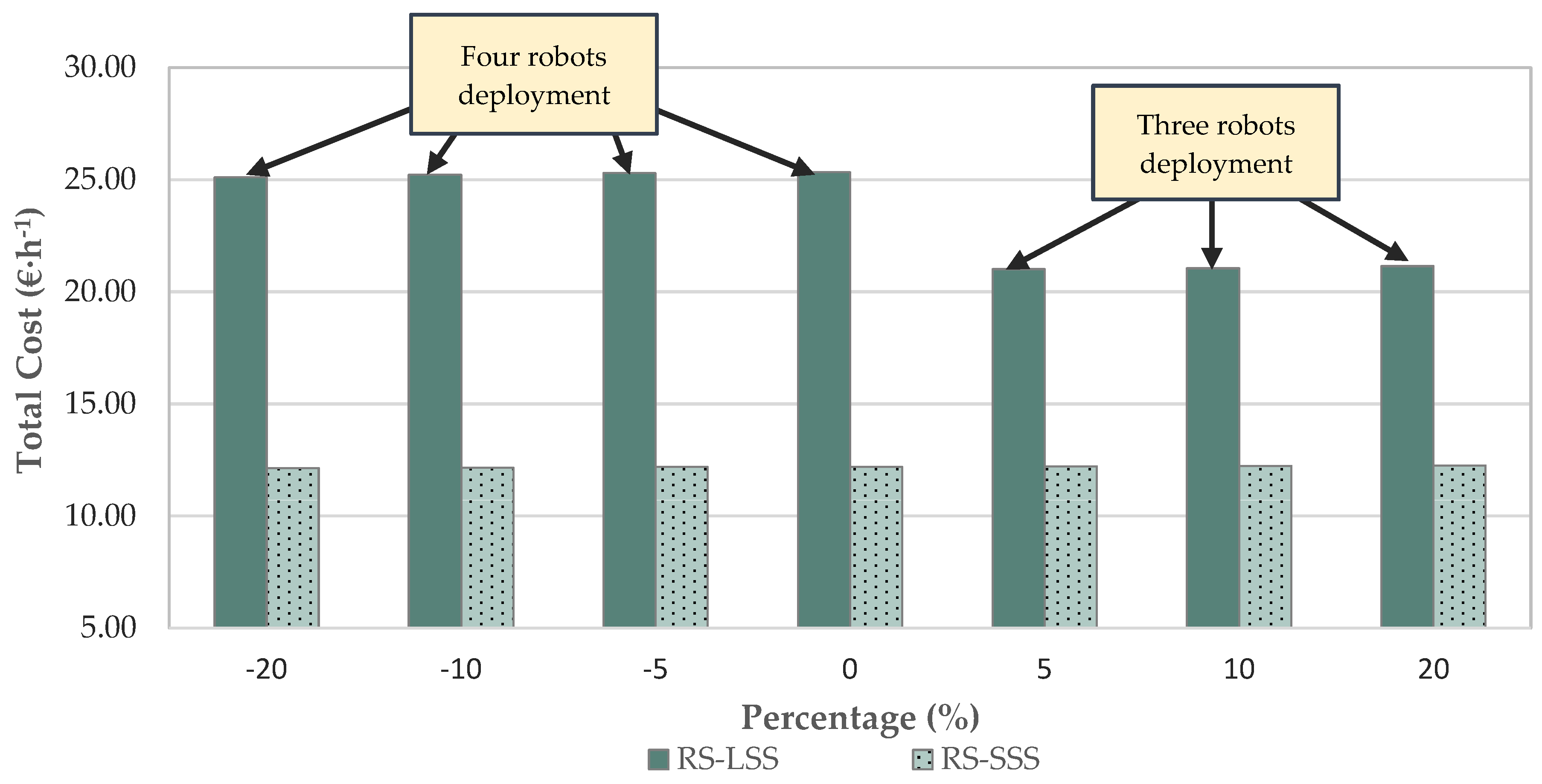
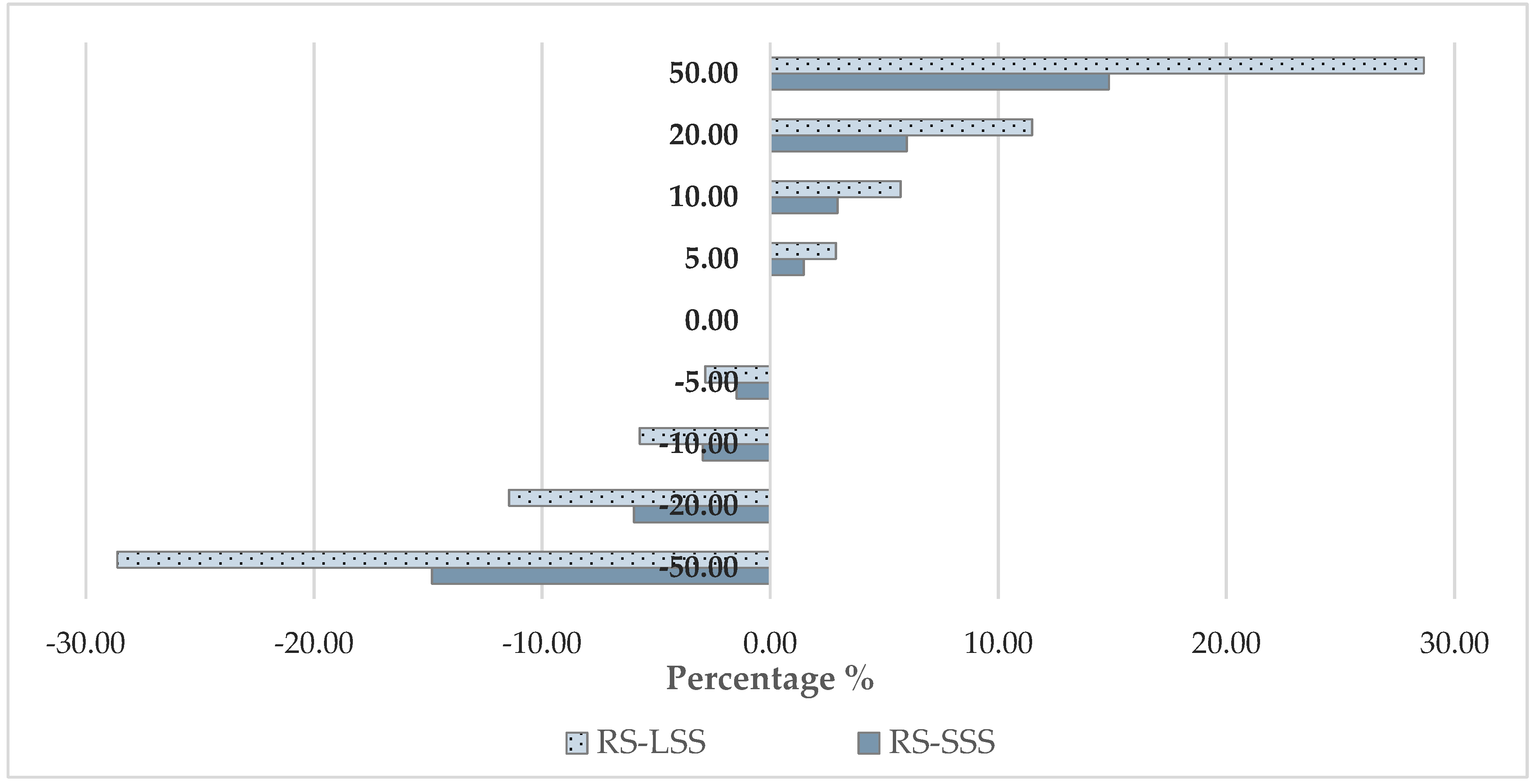
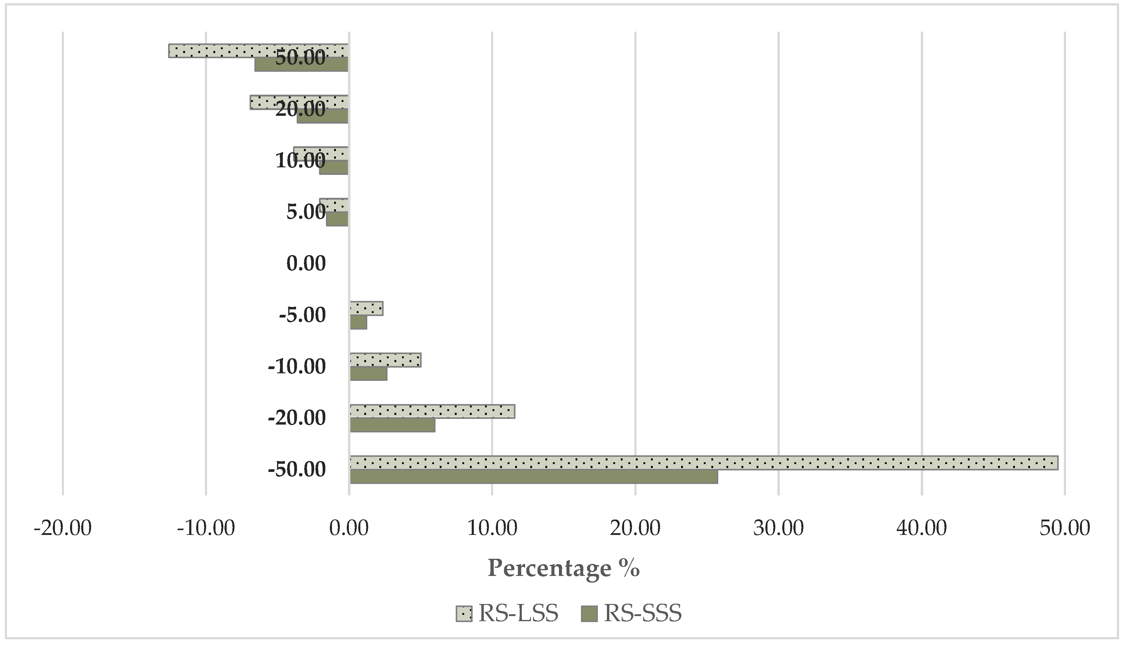
3.3. Sensitivity Analysis
4. Conclusions
Author Contributions
Funding
Conflicts of Interest
References
- Qureshi, M.O.; Syed, R.S. The impact of robotics on employment and motivation of employees in the service sector, with special reference to health care. Saf. Health Work 2014, 5, 198–202. [Google Scholar] [CrossRef] [PubMed]
- Toledo, O.M.; Steward, B.L.; Gai, J.; Tang, L. Techno-economic analysis of future precision field robots. In Proceedings of the American Society of Agricultural and Biological Engineers Annual International Meeting 2014, Montreal, QC, Canada, 13–15 July 2014. [Google Scholar]
- Hyde, J.; Engel, P. Investing in a Robotic Milking System: A Monte Carlo Simulation Analysis. J. Dairy Sci. 2002, 85, 2207–2214. [Google Scholar] [CrossRef]
- Bochtis, D.D.; Sørensen, C.G.C.; Busato, P. Advances in agricultural machinery management: A review. Biosyst. Eng. 2014, 126, 69–81. [Google Scholar] [CrossRef]
- Bongiovanni, R.; Lowenberg-Deboer, J. Precision agriculture and sustainability. Precis. Agric. 2004, 5, 359–387. [Google Scholar] [CrossRef]
- Liakos, K.G.; Busato, P.; Moshou, D.; Pearson, S.; Bochtis, D. Machine learning in agriculture: A review. Sensors 2018, 18, 2674. [Google Scholar] [CrossRef] [PubMed]
- Moradi, M.; Moradi, M.; Bayat, F. On robot acceptance and adoption: A case study. In Proceedings of the 2018 Artificial Intelligence and Robotics (IRANOPEN): the 8th Conference on Artificial Intelligence and Robotics, Qazvin, Iran, 8 April 2018; pp. 21–25. [Google Scholar]
- Mottaleb, K.A. Technology in Society Perception and adoption of a new agricultural technology: Evidence from a developing country. Technol. Soc. 2018, 55, 126–135. [Google Scholar] [CrossRef] [PubMed]
- Sørensen, C.G.; Nielsen, V. Operational analyses and model comparison of machinery systems for reduced tillage. Biosyst. Eng. 2005, 92, 143–155. [Google Scholar] [CrossRef]
- Pedersen, S.M.; Fountas, S.; Have, H.; Blackmore, B.S. Agricultural robots - System analysis and economic feasibility. Precis. Agric. 2006, 7, 295–308. [Google Scholar] [CrossRef]
- Bochtis, D.D.; Sørensen, C.G.; Busato, P.; Berruto, R. Benefits from optimal route planning based on B-patterns. Biosyst. Eng. 2013, 115, 389–395. [Google Scholar] [CrossRef]
- Jensen, M.F.; Bochtis, D.; Sørensen, C.G. Coverage planning for capacitated field operations, part II: Optimisation. Biosyst. Eng. 2015, 39, 149–164. [Google Scholar] [CrossRef]
- Rodias, E.; Berruto, R.; Busato, P.; Bochtis, D.; Sørensen, C.G.; Zhou, K. Energy savings from optimised in-field route planning for agricultural machinery. Sustainability 2017, 9, 1956. [Google Scholar] [CrossRef]
- Busato, P.; Berruto, R. Minimising manpower in rice harvesting and transportation operations. Biosyst. Eng. 2016, 151, 435–445. [Google Scholar] [CrossRef]
- Tsatsarelis, C. Agricultural Machinery Management, 1st ed.; Giachoudi Publications: Thessaloniki, Greece, 2006; ISBN 960-7425-86-3. [Google Scholar]
- Bochtis, D.; Sorensen, C.G.; Kateris, D. Operations Management in Agriculture, 1st ed.; Elsevier: Amsterdam, The Netherlands, 2018; ISBN 9780128097168. [Google Scholar]
- American Society of Agricultural and Biological Engineers (ASABE). Agricultural Machinery Management—ASAE EP496.3 FEB2006 (R2015); ASABE: St. Joseph, MI, USA, 2006. [Google Scholar]
- Bubeck, S.; Tomaschek, J.; Fahl, U. Perspectives of electric mobility: Total cost of ownership of electric vehicles in Germany. Transp. Policy 2016, 50, 63–77. [Google Scholar] [CrossRef]
- American Society of Agricultural and Biological Engineers (ASABE). Agricultural Machinery Management Data—ASAE D497.5 FEB2006; ASABE: St. Joseph, MI, USA, 2006. [Google Scholar]
- American Society of Agricultural and Biological Engineers (ASABE). Agricultural Machinery Management Data— ASAE D497.7 MAR2011 (R2015); ASABE: St. Joseph, MI, USA, 2015. [Google Scholar]
- Grimstad, L.; From, P. The Thorvald II Agricultural Robotic System. Robotics 2017, 6, 24. [Google Scholar] [CrossRef]
- Propfe, B.; Redelbach, M.; Santini, D.J.; Friedrich, H.; Characteristics, V.; Sh, M.; Mercedes, S. Cost Analysis of Plug-in Hybrid Electric Vehicles including Maintenance & Repair Costs and Resale Values Implementing Agreement on Hybrid and Electric Vehicles. Proc. 26th Int. Batter. Hybrid Fuel Cell Electr. Veh. Symp. 2012, 5, 6862. [Google Scholar]
- Ministry of Development and Competitiveness Liqid Fuel Prices Observatory. Available online: http://www.fuelprices.gr/PriceStats?prodclass=1&nofdays=7&order_by=9 (accessed on 17 December 2018).


| RS | CS-SCS Small-Scale | CS-LSC Large-Scale | ||
|---|---|---|---|---|
| Field operation parameters | Working width (m) | 1.2 | 2.6 | 6.0 |
| Speed (km h−1) | 4 | 8 | 8 | |
| Working period (day) | 12 | 12 | 12 | |
| Workability coefficient | 0.6 | 0.6 | 0.6 | |
| Working hours (h day−1) | 17 | 17 | 17 | |
| Investment and ownership parameters | Interest rate (%) | 9 | 9 | 9 |
| Inflation (%) | 4 | 4 | 4 | |
| Economic life (y) | 15 | 15 | 15 | |
| Purchase price (€) | 50,000 | 40,000 | 130,000 | |
| Implement purchase price (€) | 1000 | 3000 | 6000 | |
| Salvage value (%) | 10.9 | 10 | 10 | |
| Housing coefficient | 2.25 | 0.75 | 0.75 | |
| Insurance coefficient | 0.75 | 0.25 | 0.25 | |
| Machinery parameters | R&M * factors | - | 0.003 | 0.003 |
| - | 2 | 2 | ||
| Implement R&M factors | 0.17 | 0.17 | 0.17 | |
| 2.2 | 2.2 | 2.2 | ||
| Machine power (KW) | 3.4 | 40 | 80 | |
| Energy cost (€ KWh−1) | 0.145 | 0.496 | 0.496 | |
| Labor Cost (€ h−1) | 7.5 | 15 | 15 |
| RS-SCS Small-Scale | CS-SCS | RS-LCS | CS-LSC | |
|---|---|---|---|---|
| Field Area (ha) | 10 | 10 | 100 | 100 |
| Operation Duration (h) | 41.35 | 5.66 | 95.94 | 24.50 |
| Idle Time (h) | 20.52 | 0.86 | 175.41 | 3.68 |
| Efficiency (%) | 50.38 | 85.00 * | 54.29 | 85.00 * |
| Min requested capacity (ha h−1) | 0.082 | 0.082 | 0.82 | 0.82 |
| Actual capacity (ha h−1) | 0.24 | 1.77 | 0.26 | 4.08 |
| Number of Units | 1 | 1 | 4 | 1 |
| Capital Cost (€) | 49.19 | 14.35 | 456.48 | 145.82 |
| Depreciation Cost (€∙year−1) | 62.63 | 18.46 | 581.25 | 187.62 |
| Insurance Cost (€) | 7.91 | 0.77 | 73.39 | 7.81 |
| Housing Cost (€) | 23.72 | 2.31 | 220.17 | 23.45 |
| Repair and Maintenance Cost (€) | 25.45 | 4.11 | 236.22 | 37.18 |
| Energy Cost (€) | 10.53 | 56.93 | 109.81 | 486.73 |
| Labor Cost (€) | 325.03 | 88.92 | 754.11 | 385.32 |
| Ownership Cost (€) | 143.45 | 35.86 | 1331.30 | 364.71 |
| Operation Cost (€) | 361.01 | 149.96 | 1100.13 | 909.24 |
| Total Cost (€) | 504.47 | 185.85 | 2431.43 | 1273.95 |
© 2019 by the authors. Licensee MDPI, Basel, Switzerland. This article is an open access article distributed under the terms and conditions of the Creative Commons Attribution (CC BY) license (http://creativecommons.org/licenses/by/4.0/).
Share and Cite
Lampridi, M.G.; Kateris, D.; Vasileiadis, G.; Marinoudi, V.; Pearson, S.; Sørensen, C.G.; Balafoutis, A.; Bochtis, D. A Case-Based Economic Assessment of Robotics Employment in Precision Arable Farming. Agronomy 2019, 9, 175. https://doi.org/10.3390/agronomy9040175
Lampridi MG, Kateris D, Vasileiadis G, Marinoudi V, Pearson S, Sørensen CG, Balafoutis A, Bochtis D. A Case-Based Economic Assessment of Robotics Employment in Precision Arable Farming. Agronomy. 2019; 9(4):175. https://doi.org/10.3390/agronomy9040175
Chicago/Turabian StyleLampridi, Maria G., Dimitrios Kateris, Giorgos Vasileiadis, Vasso Marinoudi, Simon Pearson, Claus G. Sørensen, Athanasios Balafoutis, and Dionysis Bochtis. 2019. "A Case-Based Economic Assessment of Robotics Employment in Precision Arable Farming" Agronomy 9, no. 4: 175. https://doi.org/10.3390/agronomy9040175
APA StyleLampridi, M. G., Kateris, D., Vasileiadis, G., Marinoudi, V., Pearson, S., Sørensen, C. G., Balafoutis, A., & Bochtis, D. (2019). A Case-Based Economic Assessment of Robotics Employment in Precision Arable Farming. Agronomy, 9(4), 175. https://doi.org/10.3390/agronomy9040175