Article

An Integrated Yield Prediction Model for Greenhouse Tomato

College of Electronics and Information Engineering, Tongji University, Shanghai 201804, China
*
Author to whom correspondence should be addressed.
These authors contributed equally to this work.
Agronomy 2019, 9(12), 873; https://doi.org/10.3390/agronomy9120873
Submission received: 8 November 2019 / Revised: 2 December 2019 / Accepted: 5 December 2019 / Published: 11 December 2019
(This article belongs to the Special Issue Greenhouse Technology)

Abstract

:
The commonly used greenhouse crop yield prediction models today have their specific application scenarios, which may not ensure the accuracy of the results if the greenhouse environment changes. This greatly restricts their use in the greenhouse environment. To solve this problem, two widely used tomato growth models were compared in the study: TOMGRO and Vanthoor, and then an integrated model was obtained. Through the extended Fourier amplitude sensitivity test (EFAST), the model parameters were divided into three categories: optimized, fixed and ignored. In addition, Bayesian optimization was used as an optimization algorithm, through which the parameters applicable to the greenhouse can be optimized based on the greenhouse data. Compared with TOMGRO and Vanthoor, the output of the integrated model was more reasonable and universal, and the RMSE in the integrated model was 2.5974 while that in TOMGRO and Vanthoor both were over 17, reflecting the fact that the model output was closer to the actual value. According to the verification results of four-year greenhouse data, the model had high performance in predicting yield.

1. Introduction

Crop growth model is an essential part for the optimization of the cultivation management. Besides, it can also benefit the environment control. As we all know, the greenhouse environment is a complex system with multi-variables, nonlinearity, strong coupling and large inertia. The crop growth greatly affects the environment factors with the transpiration and photosynthesis. However, due to the complex mechanism and numerous parameters, the growth model has few applications in the greenhouse and the several widely used growth models are based on specific application scenarios, which is not applicable if the environment changes. The lack of growth models has led to insignificant increases in crop yields and unsatisfactory control effects in greenhouses microclimate. Therefore, there is an urgent need for a more versatile and applicable crop yield model.
Growth models mainly consist of two categories according to the principle: descriptive model and explanatory model [1,2]. The descriptive model based on the existing theoretical knowledge and practical experience, determines the correlation between the research factors through statistical regression analysis of mass crop data [3]. Based on the dynamics principle, the explanatory model describes the relationship between environmental factors, cultivation management and crop growth, morphological development and yield forming process [3].
The two types of model above have their own advantages and disadvantages, but the explanatory model is more practical to reflect the actual growth process of crops. Moreover, with the deep research on crop physiological mechanisms and the development of computer technology, the explanatory model will be a trend for crop model development. For many years, scholars have conducted extensive researches on the explanatory model of crop growth. Jones et al. [4] proposed the TOMGRO model for the growth and development of tomato, parameters of which were mainly based on crop stems. Heuvelink [5] proposed the TOMSIM model, which focused on the study of crop canopy light interception and referenced the SUSROS87 model for the accumulation of dry matter. Israel and other countries [6] developed the common-use growth model HORTISIM, which provided the effective strategies for greenhouse environmental control and management. Van Keulen [7,8] proposed the SUCROS model, which simulated the weight of dry matter in various organs of wheat using solar radiation as the main factor affecting crop growth. Ritchie et al. [9,10,11,12] proposed the CERES model, which simulated the process of crop growth, soil and water balance, as well as energy balance. This study selected two representative tomato explanatory models that can be used for yield prediction for comparison: TOMGRO and Vanthoor.
TOMGRO is a tomato growth model proposed by Jones et al., which focuses on the study of the relationship between the growth of tomato and greenhouse environmental factors such as solar radiation, temperature and C O 2 to scientifically manage and predict the whole growth process of tomato. TOMGRO describes the entire model by using seven basic crop physiological factors (leaves number, nodes number, fruit number, leaves dry weight, nodes dry weight, fruit dry weight and leaf area index), and it is the most representative model in current greenhouse tomato growth and development simulation research [13,14,15]. The principle of TOMGRO is based on the source-sink theory. The biggest weakness of TOMGRO is that it is difficult to obtain some key parameters such as the potential growth rate in the real greenhouse environment, which has restricted the scope of its application [16].
Vanthoor is a well-structured explanatory model and its simulation performance has been extensively validated in European and North American greenhouses [17]. Vanthoor is actually a greenhouse environmental system model which includes a greenhouse microclimate model and a greenhouse crop growth model. Its crop growth model uses the buffer theory and basically obtains two crop growth status results (leaf area index and dry matter) [18,19,20]. The buffer theory is more abstract than the source-sink theory, because the former is an artificially added concept. Notably, many of its variables are more affected by microclimate parameters such as temperature or average temperature rather than by crop parameters. This makes it difficult to intuitively reflect some of the physiological characteristics of crops, but relatively, the value of its variables is easy to be obtained in the greenhouse.
It can be seen from the above comparison that TOMGRO is more suitable for cultivation management of crops and Vanthoor is more suitable for environmental regulation of greenhouses. In order to get a greenhouse tomato growth model with a wider applicable scope, the above two model was compared and obtained an integrated model in this study.The model combined the strength of TOMGRO and Vanthoor, that is, it retained a large number of crop physiological parameters, and ensured the capturing of key parameters in the greenhouse as well, greatly improving the practicality of the model. However, the model alone cannot dynamically adjusted parameters according to different greenhouse environments, so combination with the sensitivity analysis and optimization algorithm should be a good way for the repeating use of the model in various greenhouses.

2. Materials and Methods

The greenhouse data was collected from the Experimental Station (318500 N, 1218330 E), of the National Facility Agricultural Engineering Technology Center of China, in Chongming County, Shanghai City, China. Tomato plants, Gorioso, were grown in a 680 m 2 , 5 m high Venlo-type glass greenhouse with numerous actuators such as the ventilation equipment (roof-windows, side-windows and fans), heating equipment (heating pumps), curtains (shading screens and energy screens), lighting equipment (high voltage sodium lamps and light-emitting diodes) and irrigation equipment. The greenhouse contains eighteen rows of tomato crop. Crop planting density was 2.5 plants/m 2 .
The data collection began on September 20 and ended on December 28 each year (2014–2018). During the period, the side branches of tomatoes were cut off regularly, only the main stem were kept. The harvested fruit was weighed manually and recorded its weight daily. The crop was grown in the organic substrate (Rice husk charcoal), and sufficient irrigation was performed daily with the nutrient solution through the drip. Greenhouse climate data such as temperature (T, C ), C O 2 concentration ( C O 2 , ppm), photosynthetically active radiation ( P A R , μ mol/m 2 /s), humidity (H, %) and so on were recorded every hour by sensors.

2.1. Integrated Model

The main difference between TOMGRO and Vanthoor is that the division of the growth stages in TOMGRO is mainly based on the number of plant nodes, while that in Vanthoor is based on the temperature. In addition, the main calculation time scale in TOMGRO is days, while that in Vanthoor is seconds. Though based on different growth theories, TOMGRO and Vanthoor are similar in the structure of computing the net dry matter. By comparing the two models, an integrated model was obtained, which can be summarized as the following five steps:
(1)
Dividing crop organs into different age classes.
(2)
Calculating the amount of dry matter provided by the environment: SUPPLY.
(3)
Calculating the amount of dry matter required by crops: DEMAND.
(4)
Comparing SUPPLY and DEMAND to screen out two situations: oversupply and undersupply.
(5)
Obtaining the final change rate of net dry matter, according to different supply and demand situations.
Based on the five steps, the integrated model is described in detail as below:
Step 1: dividing age classes:
Consistent with TOMGRO and Vanthoor, the integrated model divided crop organs into different age classes that crop physiological characteristics in the same age group were considered the same. The physiological age of the crop took reference to the idea of TOMGRO, which is described by the current number of nodes, in other words, the number of crop organs in a certain age class is related to the number of crop nodes. Taking the age group i as an example, the rate of change in the number of stems ( N ˙ S ( i ) ), leaves ( N ˙ L ( i ) ) and fruits ( N ˙ F ( i ) ) was as shown in Equations (1)–(3):
N ˙ S ( i ) = G E N R S · n P l a n t s r L · n F · N S ( 1 ) i = 1 N S ( i 1 ) N S ( i ) · r L · n F 1 < i < n F N S ( i 1 ) · r L · n F i = n F
N ˙ L ( i ) = G E N R L · n P l a n t s r L · n F · N L ( 1 ) i = 1 N L ( i 1 ) N L ( i ) · r L · n F 1 < i < n F N L ( i 1 ) · r L · n F P L i = n F
N ˙ F ( i ) = G E N R F · n P l a n t s · R c r F · n F · N F ( 1 ) i = 1 N F ( i 1 ) N F ( i ) · r F · n F 1 < i < n F N F ( i 1 ) · r F · n F P F i = n F ,
where i represented the i-th age group. The newest crop organs were in the first group and the oldest ones in the last group. G E N R S , G E N R L and G E N R F are the appearance rate of new nodes, leaves and fruits respectively ( n o . / p l a n t / d ), n P l a n t s is the plant density ( n o . / m 2 ), R c is the ratio of supply and demand, r L and r F are the development rate function of leaves ( n o d e s ) and fruit respectively ( 1 / d ), n F is the number of organ age classes, N S ( i ) , N L ( i ) and N F ( i ) are the number of nodes, leaves and fruits in the i-th age class respectively ( n o . / m 2 ), and P L and P F are the leaves and fruit mortality respectively ( n o . / m 2 / d ).
According to Jones et al. (1991), the appearance rate of new nodes was G E N R S = G E N R A T · F N ( T ) · F ( C O 2 ) , in which G E N R A T is a constant depending on tomato varieties. However, Cooman et al. (2006) [21] stated that G E N R A T is a linear function related to the number of stems. Given that the data of nodes in the conditions of specific temperature and humidity cannot be obtained in the actual greenhouse, and relevant studies [22] found that C O 2 inhibition function in TOMGRO had little effect on the appearance rate of the nodes, the integrated model used the calculation equation of the nodes as shown in Equation (4). The appearance rate of fruit in Vanthoor: G E N R F = a + b · T C a n 24 is a linear function related to the daily average temperature. Temperature is a parameter that indirectly reflects crop growth, so it was much more inaccurate than that in TOMGRO. Therefore, the equations of stems appearance rate ( G E N R S ), leaves appearance rate ( G E N R L ) and fruit appearance rate ( G E N R F ) in the integrated model were finally shown in Equations (4)–(6):
G E N R S = a g + b g · N S · F N ( T )
G E N R L = G E N R F 1 + T P L
G E N R F = G E N R S · F P N ,
where a g and b g are function coefficients of organ appearance rate, F N ( T ) is the temperature inhibition function, T P L is the ratio of new trusses to new leaves, and F P N is the ratio of new fruit to new nodes.
A set of experimental results of leaves and fruit development rates at different temperatures were given in TOMGRO, and the development rate in Vanthoor and Cooman was the linear function related to daily average temperature. Therefore, it was concluded that the linear function of daily average temperature was more accurate when characterizing the development rate, so the development rate of leaves ( r L ) and fruit ( r F ) in the integrated model is shown in Equations (7) and (8):
r L = a r L + b r L · T d
r F = a r F + b r F · T d ,
where a r L and b r L are function coefficients of leaf development rate, a r F and b r F are function coefficients of fruit development rate and T d is the daily average temperature ( C ).
When the leaf area index (LAI) exceeded the critical value (XLAIM) in TOMGRO, the mature leaves fell off (the last age class) and the pruning operation (all age groups) was carried out; when LAI exceeded XLAIM in Vanthoor, the extra leaf carbohydrates were totally subtracted. Therefore, a leaf mortality ( P L ) equation of leaves was proposed as shown in Equation (9) by combining the leaf mortality of the above two models. It simulated the leaf death and pruning based on age groups and maximum LAI; and the older leaves fell off and were trimmed more possibly. Although TOMGRO proposed the concept of fruit mortality, no specific equation and description were given, and there was no concept of fruit mortality in Vanthoor. Therefore, the study adopted Cooman’s fruit mortality ( P F ) equation, a linear function of R c , as shown in Equation (10):
P L ( i ) = N L ( i ) · 1 X L A I M L A I · k · i L A I X L A I M k · i 0 L A I < X L A I M k · i
P F = a P F b P F · R c ,
where X L A I M was the critical LAI ( m 2 / m 2 ), a P F and b P F were the function coefficients of fruit mortality, and k was the regulatory factor.
Step 2: calculating supply:
Supply represented the amount of carbohydrates produced by crops after absorbing external energy. Accordingly, this step was mainly used to calculate the photosynthesis rate and respiration rate of crops. Since most of the results from the photosynthesis models were similar, the integrated model here was consistent with TOMGRO. Equations (11)–(13) showed the calculation formula of SUPPLY, photosynthesis rate (A) and respiration rate ( R m ):
S U P P L Y = E · A R m
A = D P max K ln ( 1 m ) P max + ε · K · P P F D ( 1 m ) P max + ε · K · PPFD · e K · L A I
R m = Q 10 0.1 ( T 20 ) R E S P L · W L + W S + R E S P F · W F ,
where E is the conversion efficiency ( g { D M } / g { C H 2 O } ), D was the unit conversion factor ( g { C H 2 O } / u m o l { C O 2 } / 3600 ), P max is the maximum photosynthesis rate ( μ m o l / m 2 / s ), K is the light extinction coefficient, m is the light transmission coefficient, ε is the quantum efficiency ( m o l { C O 2 } / m o l { p h o t o n s } ), P P F D is the photosynthetic photon flux density ( μ m o l / m 2 / s ), Q 10 was the sensitivity to temperature, R E S P L and R E S P F are the relative respiration requirement of leaves and fruit respectively ( g { C H 2 O } / g { D M } / d ), and W L , W S and W F were dry matter of the leaves, nodes and fruit respectively ( g / m 2 ).
Step 3: Calculating demand:
Demand represented the amount of carbohydrates required for the growth of crop organs. TOMGRO was consistent with Vanthoor in the fruit dry matter demand. Because Vanthoor did not set the age groups of leaves and nodes, it had no formula to calculate the required volume of the leaves and nodes. Therefore, the integrated model was consistent with TOMGRO in the calculation of the leaves and nodes. In addition, the C O 2 inhibition function had little effect on the results in the step, and there was no C O 2 inhibition function in Vanthoor, so the function was removed in the integrated model. The dry matter demand of stems ( S d e m ), leaves ( L d e m ) and fruit ( F d e m ) and leaf area change rate ( A ˙ L P ) were as shown in Equations (14)–(17):
S d e m ( i ) = L d e m ( i ) · F R S T M · N S ( i ) N L ( i )
L d e m ( i ) = ( 1 + F R P E T ) · A ˙ L P ( i ) S L A
F d e m ( i ) = P O F ( i ) · F N ( T ) · N S ( i )
A ˙ L P ( i ) = N L ( i ) · P O L ( i ) · F N ( T ) ,
where F R S T M is the ratio of node growth rates to leaf growth rates, F R P E T is the ratio of petiole weight to blade weight, S L A is the average specific leaf area ( m 2 / g { D M } ), P O F ( g { D M } / f r u i t / d ) and P O L ( g { D M } / l e a f / d ) are the potential growth rate of fruit and leaves respectively (Equations (18) and (19)).
The experimental data of the potential growth rate of fruit and leaves at different organ development stages were given in TOMGRO, and the empirical equation at the development stages was used in Vanthoor. They were more precise than the discrete data in TOMGRO, so using a combination of Vanthoor and other related researches [21,23], the potential growth rates of fruit ( P O F ) and leaves ( P O L ) in the integrated model were as shown in Equations (18) and (19):
P O F ( i ) = 0.0458 · a F · e b F S F D c F · b F · e b F S F D c F
P O L ( i ) = 1.248 · a L · e b L S L D c L · b L · e b L S L D c L ,
where a F , b F and c F are the coefficients in the potential growth rate function of fruits, S F D is the fruit development stage, a L , b L and c L are the coefficients in the potential growth rate function of leaves, and S L D is the leaf development stage.
Step 4 Comparing supply and demand:
In TOMGRO, the supply–demand ratio was compared daily to determine the R c , so that the actual organ dry matter growth rate was obtained, while Vanthoor used the idea of the cumulative amount of difference between supply and demand to determine whether to distribute dry matter, that is, it only carried out dry matter distribution when the supply reached a certain level. In comparison, the processing in TOMGRO was finer, so the integrated model used the idea of TOMGRO to handle the relationship of supply and demand. The supply–demand ratio ( R c ) and the actual dry matter growth rate of fruit ( g F ), stems ( g S ) and leaves ( g L ) were shown in Equations (20)–(23):
R c = S U P P L Y D E M A N D
g F ( i ) = F d e m ( i ) R c 1 F d e m ( i ) · R c 0 R c < 1
g S ( i ) = S d e m ( i ) R c 1 S d e m ( i ) · R c 0 R c < 1
g L ( i ) = L d e m ( i ) R c 1 L d e m ( i ) · R c 0 R c < 1
Step 5: Calculating dry matter:
TOMGRO and Vanthoor had similar structure in calculating the rate of change of dry matter: the dry matter change rate in a specific age group = the actual dry matter growth rate in the current age group + the dry matter coming the previous age group − the dry matter entering into the next age group. So the change rate of the dry matter of stems ( W ˙ S ), leaves ( W ˙ L ) and fruit ( W ˙ F ) in the integrated model were shown in the following Equations (24)–(26):
W ˙ S ( i ) = g S ( i ) + W S ( i 1 ) W S ( i ) · r L · n F
W ˙ L ( i ) = g L ( i ) + W L ( i 1 ) W L ( i ) · r L · n F
W ˙ F ( i ) = g F ( i ) + W F ( i 1 ) W F ( i ) · r F · n F .
See from the above description of the integrated model, the model used the shared structure of the source-sink theory and the buffer theory. The idea of dividing the age classes according to the number of nodes in TOMGRO was mainly adopted. With the rapid development of technologies such as computer vision, TOMGRO used the more intuitive data of nodes to reflect the state of crop growth, providing an interface for subsequent application of computer vision in greenhouse control such as fruit picking and pest warning, while the temperature in Vanthoor can only reflect the growth of crops indirectly. In addition, the integrated model provided empirical equations for parameters that were hard to be obtained based on other relevant models and studies such as Vanthoor, and optimized some of the content in the growth model, such as removing the C O 2 inhibition function when calculating the appearance rate of the new nodes and optimizing the leaf area processing function, etc.

2.2. Sensitivity Analysis

The integrated model should first find the parameters that have a great impact on the output and change with the greenhouse environment before optimization in a specific greenhouse environment. The main principle of finding the parameters to be optimized is to obtain these parameters by changing the input parameters, and the analysis of the influence degree of the model parameters on the model output generally depends on sensitivity analysis.
The sensitivity analysis is divided into two major categories: local sensitivity analysis and global sensitivity analysis [24,25]. The local sensitivity analysis is mainly applicable to scenes with no influence between the parameters in the model, while global sensitivity analysis is applicable to scenarios where the parameters in the model affect each other, and the related study [26,27] shows that global sensitivity analysis has better effect on crop model parameters analysis than local sensitivity analysis. Most of the parameters in the integrated model are coupled to each other, so the global sensitivity analysis was used in the study.
The global sensitivity analysis is composed of Morris method, sobol method, FAST method, EFAST method [28,29,30,31], etc. Currently, sobol and EFAST method are more commonly used. Because the EFAST method combines the FAST and sobol methods, it has the advantages of stability, high precision and fast calculation compared with other methods [32,33]. Therefore, the EFAST method is used to analyze the sensitivity of the relevant parameters in the integrated model.
According to the data collection table (see Appendix A) of the integrated model in the study, 13 parameters were selected for sensitivity analysis (because the parameters POL and POF which determine the sink-strength were one-dimensional vectors of the crop age class, it was difficult to conduct sensitivity analysis in the study. However, according to related studies [23] and simulations, POF has a great influence on the yield, so it needs to be optimized by default). The parameter range was set according to the average value of the parameters provided by Cooman [21], and it took reference to the +/−10% principle [34,35,36]. In this range, the parameters were evenly distributed [37,38], as shown in Table 1.

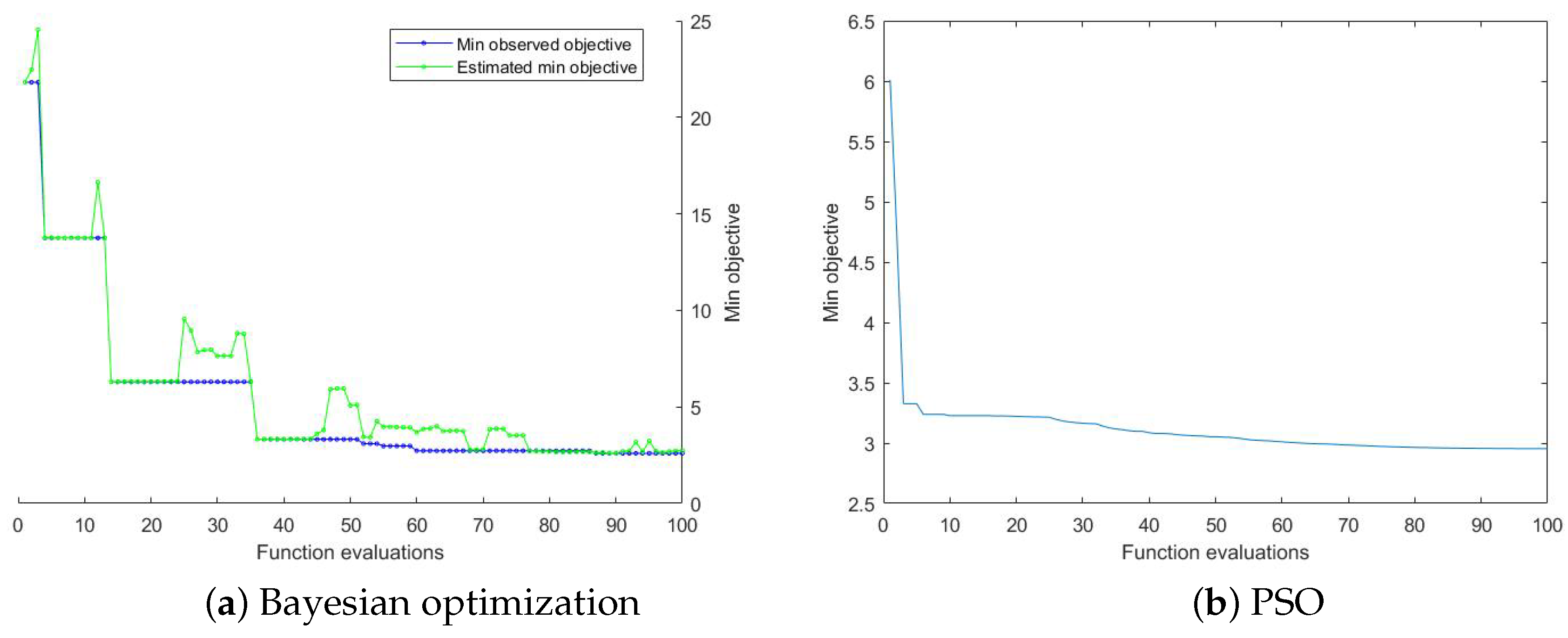
2.3. Optimization Algorithm

After the integrated model was determined and sensitivity analysis was conducted, parameters optimization was carried out. It covered three cases: (1) the input and output data corresponding to the parameters to be optimized can be obtained in reality.In this case, the actual data can be directly used for optimization; (2) the input and output data corresponding to the parameters to be optimized cannot be actually obtained, but can be obtained indirectly from other parameters.In this case, the actual data can also be used for optimization; (3) The input and output data of the parameter to be optimized cannot be actually obtained. This requires optimization by soft measurement, such as state-based estimation. The sensitive parameters in the integrated model were not the first case. Taking the r F parameter as an example, it actually indicated the transfer rate of the number of fruits between the age groups.In TOMGRO, it was obtained in a laboratory environment based on a large number of data such as the fruit dry matter, but it was impossible to obtain them in a real greenhouse. Therefore, the method of indirect parameter optimization was adopted. Take the parameter a r F and other parameters in the equation where r F is located (see below) as an example.
r F = a r F + b r F · T d
N ˙ F ( i ) = G E N R F · n P l a n t s · R C r F · n F · N F ( 1 ) i = 1 N F ( i 1 ) N F ( i ) · r F · n F 1 < i < n F N F ( i 1 ) · r F · n F P F i = n F
Therefore, the above equation was calculated to obtain the relationship between the total number of fruits at the current moment and r F .
At specific time t, the total number of fruits was the sum of the number of fruits in all age groups:
N F t = i = 1 n F N F t ( i ) .
From Equations (28–(30) can be calculated:
N F t = N F t 1 + G E N R F · n p l a n t s · R c .
It was found from Equation (30) that r F disappeared during the calculation, that is, r F was only an intermediate variable, which had no effect on the total number of fruits at a certain moment. In fact, Equation (30) indicated that the current number of fruits was the number of fruits in the previous moment plus the number of new fruits. This physical meaning can also verify the reason why r F disappeared.
What r F really affected was the number of mature fruits.The number of mature fruits was N F (10) (assuming the total age groups are 10), and it was related to the number of fruits in the previous age group, while the number of fruits in the previous age group was actually not available in the real greenhouse. It can be found that it was difficult to optimize the parameters locally in the model, therefore, the study finally selected the model’s microclimate as input and the mature fruit yield as the output, and used the overall growth model for parameter optimization. There were two reasons for this choice: 1. Microclimate and mature fruit yield data can be obtained in the real greenhouse; 2. all the sensitive parameters for yield can be optimized at one time.
Therefore, the optimized objective function was set as the RMSE between the predicted yield and the actual yield in the whole growth cycle, as shown in Equation (31).
f B O = 1 n i = 1 t W M ( i ) W M A ( i ) 2 ,
where W M was the simulated yield, W M A was the actual yield, n was the simulated days.
Take the commonly used optimization algorithm particle swarm optimization (PSO) as an example, it took more than one minute for the integrated model to run once (it simulated crop growth for 100 days on a i7-7700HQ PC with 8 GB RAM), and the time multiplied the iterations and populations quantity to get a very long optimization time. This problem was fundamentally a costly optimization problem, that is, it took a long time to calculate the objective function. Usually, the solution to such problem in the field of evolutionary computing is to use a surrogate model, or Bayesian optimization. Bayesian optimization is often used to calculate the target value that is costly and time-consuming [39]. It is equivalent to introducing domain knowledge during the search process, so the search efficiency is much faster than that of grid and random search.
In this paper, the Bayesian optimization selected the LCB function as acquisition function (Equation (32)) and the iterations were set to 100.
LCB = μ ( x ) + k σ ( x ) ,
where μ ( x ) is the mean value of a certain point, σ ( x ) was the variance of a certain point, and k was the adjustment parameter.
In Equation (32), the mean represented the final expected effect of the point; the smaller the mean value, the better the final index of the model. The variance indicated the uncertainty of this point; the larger the variance was, the more the point should be explored. The algorithm steps for Bayesian optimization were shown in Algorithm 1:
Algorithm 1: Outline. Steps of Bayesian optimization algorithm.
Input: Microclimate data (T, C O 2 , P A R ), mature fruit yield ( W M A ), and the range of variables.
Output: The best vector (solution).
Step 1: Randomly sample n points in the sample space, and calculate the posterior probability distribution of the first n points by Gaussian process regression to obtain the expected mean and variance of each hyperparameter at each value point.
Step 2: Get the next sample point according to the acquisition function (Equation (32)), and calculate the objective function value of the sample point (Equation (32)).
Step 3: Determine whether the accuracy requirement or the number of iterations is reached. If the condition is not met, add the sample points to the sample point set, repeat the above steps; and if the conditions are met, stop the iteration.

3. Results and Discussion

The equipment used in the relevant simulations and experiments is an Intel® C o r e T M i7-7700HQ, armed with a 2.80 GHz processor and 8.00 GB in RAM; the OS of the computer is W i n d o w s T M 10 Professional Edition, and the machine is equipped with the M A T L A B T M R2017a version software.

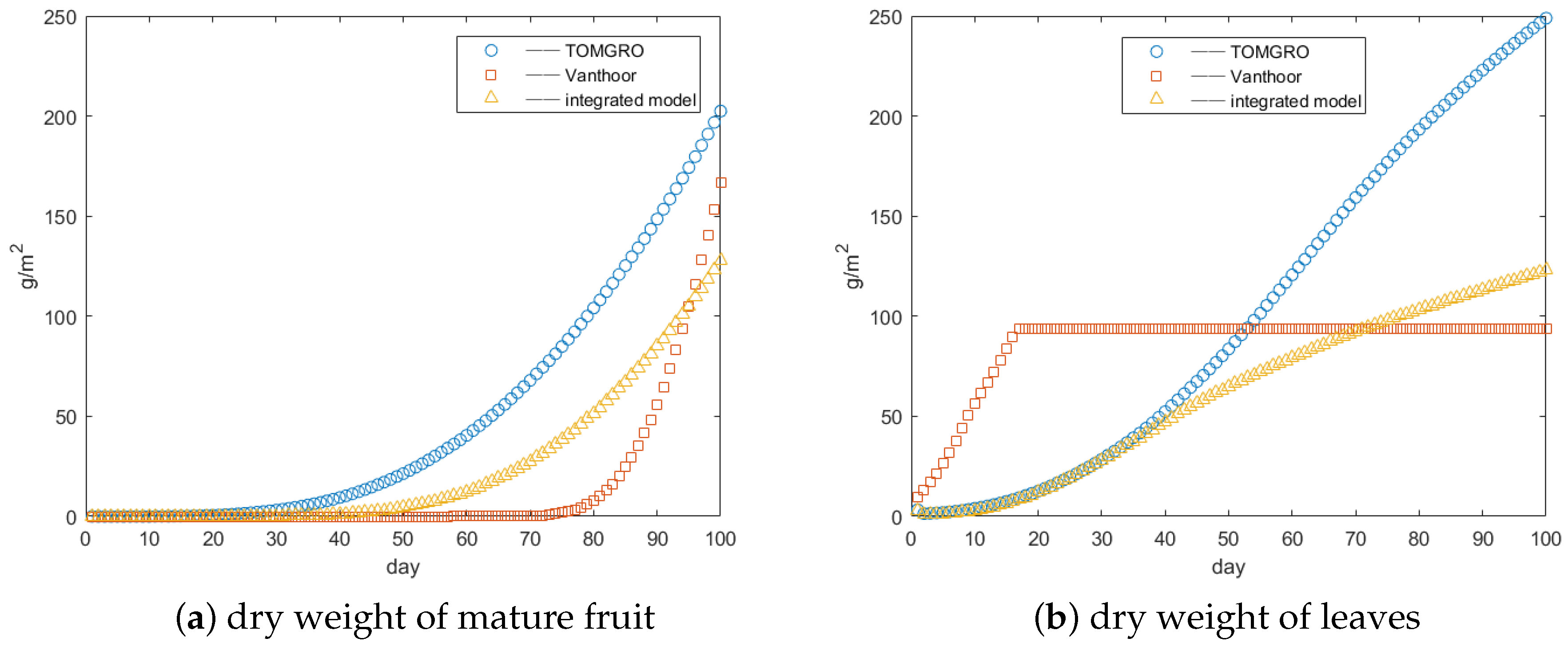
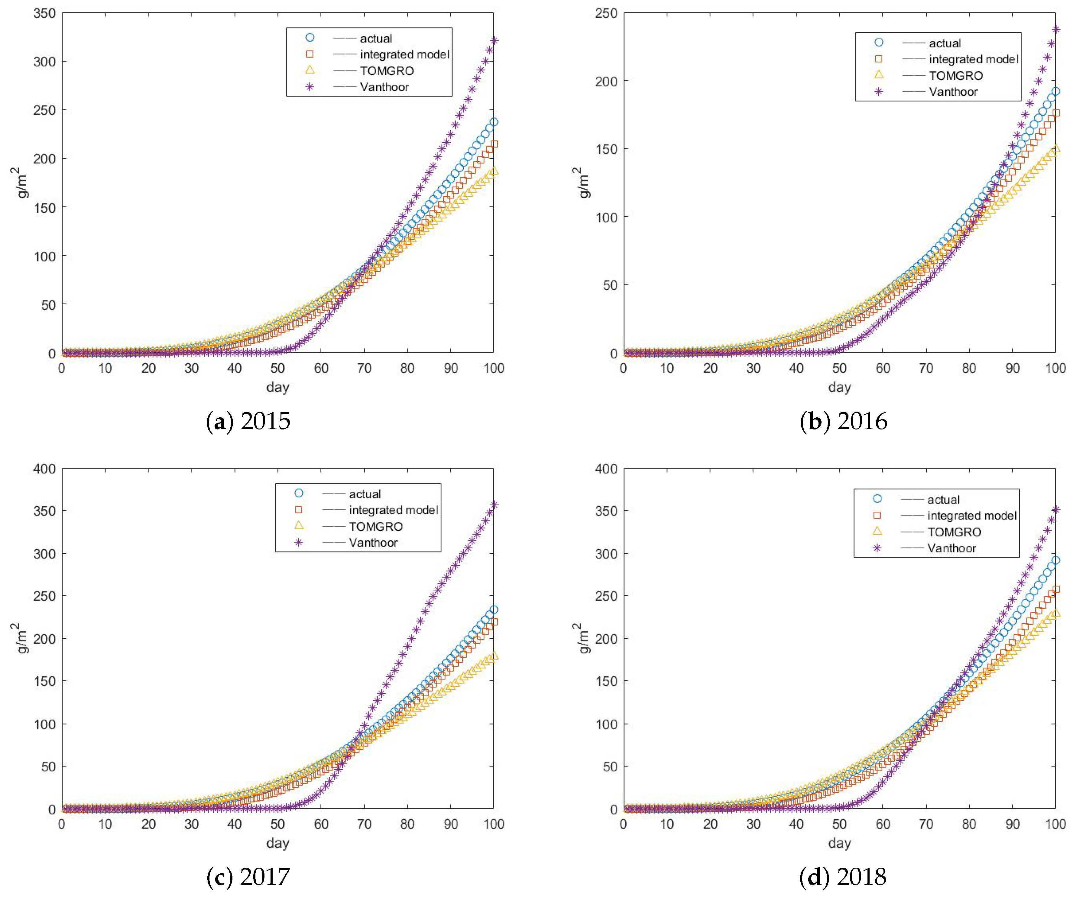
3.1. Integrated Model Validation

For the output of the integrated model, such as the dry weight of mature fruit and leaves, the comparison among the integrated model, TOMGRO and Vanthoor was shown in Figure 1.
According to Figure 1, the dry weight of mature fruits of the integrated model was within the range of the output of TOMGRO and Vanthoor. The dry weight of leaves in the integrated model changed more gently compared to TOMGRO when the leaf area approached the designated maximum (the maximum leaf area index was consistent, both were set to 2 m 2 / m 2 ), while it was different from the dry weight of leaves in Vanthoor which remained completely constant after a certain time, and was closer to the actual situation. Figure 1 indicated the rationality of the results of the integrated model.

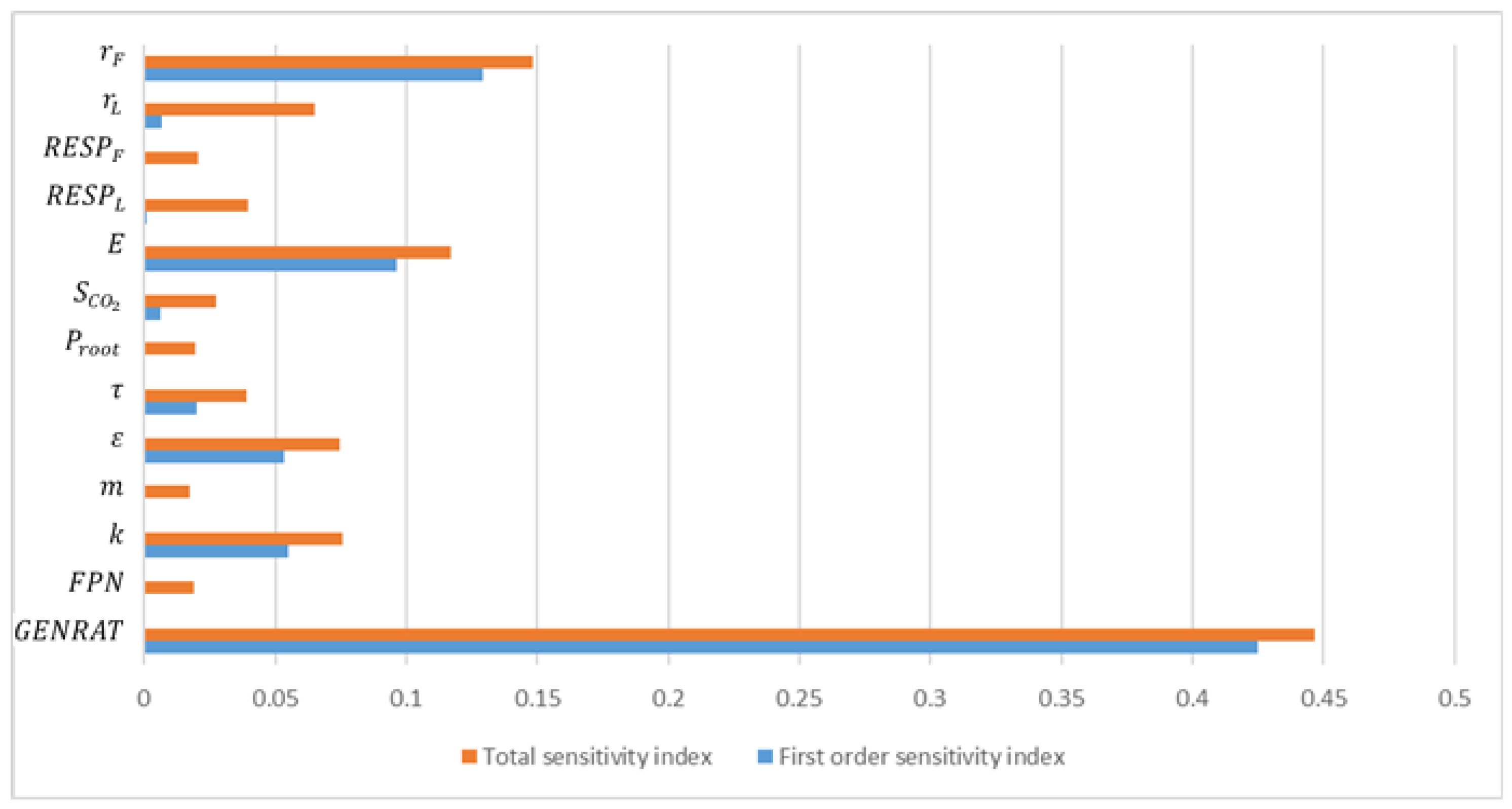
3.2. Parameter Analysis Results

After the integrated model was obtained, the parameters to be optimized were sorted out through sensitivity analysis and then the optimization algorithm was carried out.In this paper, EFAST was selected as the sensitivity analysis algorithm. The table and figure of sensitivity analysis results were shown in Table 2 and Figure 2:
A parameter with sensitivity index exceeding 0.1 is generally considered as the sensitive parameter [40]. The above figure indicated that among the 13 parameters selected, G E N R A T , E and r F had over 0.1 sensitivity index, suggesting these parameters had a significant impact on the growth model. G E N R A T represented the maximum appearance rate of new nodes, which had a direct effect on the number of nodes, and the relevant studies [4] indicated that its value was related to tomato varieties meaning that re-optimization on different tomato varieties should be arranged to improve the accuracy of the model. E represented the conversion coefficient of photosynthesis assimilation rate to dry matter accumulation rate, which had a direct impact on S U P P L Y , but its value was fixed in TOMGRO, so no extra optimization was conducted. r F was the fruit development rate which had a direct impact on the number of fruits. Its value was related to tomato varieties, meaning that re-optimization on different tomato varieties should be arranged to reduce errors of the model like G E N R A T . In order to reduce the model error, the above two sensitive parameters ( G E N R A T and r F ) should be optimized. Among the remaining parameters, it was found that the sensitivity value of some parameters which had been expected to be optimized [4] was very low, such as F P N , m, τ , P r o o t , etc. Although these parameters changed with the greenhouse structure, the type of crops, etc., all these changes had little influence on the final results of the model. Therefore, these parameters can be considered as fixed, and their values are set as recommended values or average values according to some studies [21]. The last remaining value S C O 2 was a fixed value, and its impact on the final results of the model was very small, verifying the idea of ignoring this parameter in the previous section.
Therefore, according to the above results, for the goal of yield, the parameter processing results were obtained as below:
Finally, combining the results in Table 3 and the parameter that need to be optimized by default, there are three parameters should be optimized, namely G E N R A T , r F , and P O F . According to Equations (4), (8) and (18), the following parameters for optimization was obtained, and the default recommended values were attached, as shown in Table 4. The Appendix Data Collection Table showed the information of the remaining parameters in the model.

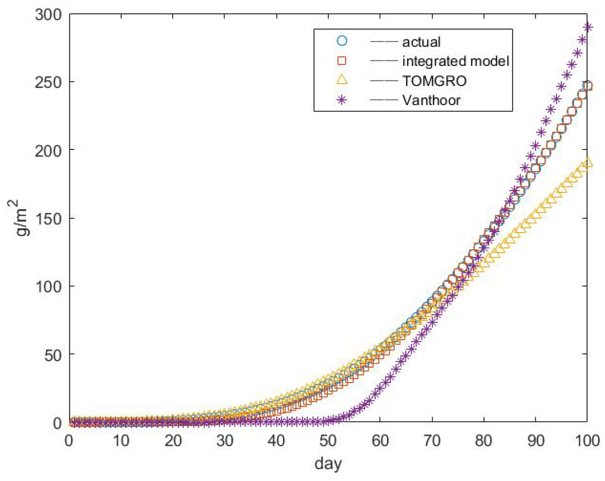
3.3. Results of Yield Prediction

The parameters obtained after the sensitivity analysis of the model can be optimized based on greenhouse data, and the results of the yield prediction can be obtained finally.
The microclimate data was selected from Chongming Greenhouse in 2014 (the data selected from September 20 to December 28, an actual growth cycle of Chongming Greenhouse). The range of parameters to be optimized was +/−20% from the default value (After comparative testing, 20% was a reasonable and better range). The optimization results of the Bayesian optimization algorithm were shown in Table 5.
The RMSE changed in line with the iterations in Bayesian optimization algorithm and PSO were seen as follows:
It can be seen from the results in the Figure 3 that by using Bayesian optimization to identify the growth model parameters, the RMSE of the yield were 2.5217, 2.5974, 2.2309, 2.5974 and 2.5096 (ran five times continuously to reduce the impact of randomness, and the worst result was selected), The RMSE of PSO were 2.9534, 4.0855, 2.0732, 2.7776 and 3.5322. It can be seen that most of the RMSE of PSO were higher than the worst result of Bayesian optimization (except 2.0732), and the results of PSO were not as stable as the results of Bayesian optimization (a large RMSE: 4.0855 appeared in the results). In addition, the runtime of the Bayesian optimization was only about 2 h, 1/10 the time of the PSO. The reason was that the information of all previous iterations was utilized for the next search in the Bayesian optimization algorithm, making it more efficient than the grid and random search.
The optimized parameters were re-substituted into the model to compare with the actual yield, TOMGRO and Vanthoor, as shown in Figure 4:
In Figure 4, the RMSE between the TOMGRO and the actual yield was 17.2154, the RMSE of Vanthoor was 17.6157, and the RMSE of the model proposed in this paper was 2.5974. It was not hard to find that compared with the output of TOMGRO and Vanthoor (both with calibrated parameters), the output of the model proposed in this paper was closer to the actual yield. This proved that the model had higher accuracy in predicting greenhouse crop yield.
The integrated yield prediction model proposed in this paper also had the ability to “memorize”, meaning that after one parameter optimization in a particular greenhouse, the model can run accurately in the greenhouse for a long time without the second-time optimization. After conducting the optimization algorithm with the data of Chongming Greenhouse in 2014, the study used other growth cycle data (Chongming Greenhouse from 2015 to 2018) as a verification set to validate the scheme. The results were shown in Figure 5.
It can be seen from Figure 5 that after using the optimized parameters (tuned with the data of Chongming Greenhouse in 2014),the model output can approximate the actual yield well when different climate data (2015 to 2018) was input. By comparing with TOMGRO and Vanthoor, the RMSE of the integrated model, TOMGRO and Vanthoor was 9.7508, 15.4559 and 27.0760 in 2015, 6.7849, 13.6584 and 14.5267 in 2016, 7.4368, 16.9145 and 49.4001 in 2017, and 14.5421, 18.7890 and 22.0839 in 2018. Therefore, this proved once again that the integrated model combined with the optimization algorithm had a high accuracy in predicting yield. The reason was that the model combined the advantages of TOMGRO and Vanthoor. Compared with Vanthoor, it had a more detailed simulation of the crop mechanism, so the model output will not deviate too much from the actual yield. Compared with TOMGRO, it had more accurate parameters, so its output can be closer to the actual yield after the optimization algorithm.

4. Conclusions

To solve the problem of poor reusability of the existing greenhouse crop yield prediction models, an integrated yield prediction model for greenhouse tomato was proposed in the study, which included an integrated model, sensitivity analysis and an optimization algorithm. The summary of this paper was as follows:
(1) By analyzing the two representative growth theories of source-sinkand buffer on the basis of the research of TOMGRO, Vanthoor and related growth models, an integrated model for greenhouse tomato was proposed. Through the comparison of the model output, it was found that the output of the integrated model is reasonable and compared with TOMGRO and Vanthoor, it was more general.
(2) Then, the sensitive parameters which have a great influence on the model output and vary with the greenhouse environment should be determined by sensitivity analysis, and they were marked as parameters to be optimized. Other parameters were classified into fixed and ignored.
(3) Bayesian optimization was then used as the optimization algorithm. The RMSE of the yield in the whole growth cycle was taken as the objective function, and the actual greenhouse data was used for parameter optimization. The comparison results of the model output showed that the predicted value of the integrated model after parameter optimization was closer to the actual yield than TOMGRO and Vanthoor, indicating that the integrated yield prediction model has good performance in predicting yield.
(4) One-year greenhouse data was input to conduct parameter optimization for the integrated model. The model output can well track the actual yield for the next four years, compared to TOMGRO and Vanthoor, which proved once again that the model had high accuracy in predicting the yield, and indicated that once the greenhouse parameter optimization was carried out, the model can accurately predict the yield in the greenhouse for a long period of time.

Author Contributions

Conceptualization, L.X. and R.W.; methodology, R.W. and D.L.; software, D.L.; resources, L.X.; writing—original draft preparation, D.L.; writing—review and editing, L.X. and R.W.

Acknowledgments

This work was supported in part by National Natural Science Foundation of China (Grant No. 61573258), Shanghai Municipal Science and Technology Commission Innovation Action Plan (Grant No. 17391900900), U.S. National Science Foundation’s BEACON Center for the Study of Evolution in Action (DBI-0939454) and Shanghai Agriculture Applied Technology Development Program, China (Grant No. G2018-3-2).

Conflicts of Interest

The authors declare no conflict of interest.

Appendix A

Table A1. Data collection table.
AccessSymbolPhysical MeaningUnitRemarks
Sensor P A R Indoor photosynthetically active radiation μ m o l / m 2 / s -
C O 2 Indoor C O 2 concentration p p m -
TIndoor temperature C -
variables F P N Fruit initiated per new node--
KLight extinction coefficient-The values of the parameters are related to geography and greenhouse structure
mLeaf light transmission coefficient-
ϵ Leaf quantum efficiency m o l { C O 2 } / m o l { p h o t o n s }
τ Carbon dioxide use efficiency μ { p h o t o n s } / m 2 / s / 10 6 p p m { C O 2 }
Empirical formula F N ( T ) Temperature inhibition function- 0.20776 + 0.02043 T 24 / ( 0.20776 + 28 0.02043 )
P O L ( i ) Potential growth rate of leaves g { D M } / l e a f / d 0.0458 a L e b L S L D c L e b L S L D c L
P O F ( i ) Potential growth rate of fruit g { D M } / f r u i t / d 1.248 a F e b F S F D c F e b F S F D c F
r L Leaves development rate 1 / d a r L + b r L T d
r F Fruit development rate 1 / d a r F + b r F T d
G E N R A T Maximum rate of node initiation n o d e / p l a n t / d a g + b g N S t e m
P L Leaves mortality l e a f / m 2 / d L A I X L A I M i · k : N L ( i ) · 1 X L A I M L A I · i · k ; L A I < X L A I M i · k : 0
P F Fruit mortality f r u i t / m 2 / d a p F b p F · R c
FixedDConversion efficiency g { C H 2 O } / u m o l { C O 2 } / 3600 2.593
EUnit conversion factor g { D M } / g { C H 2 O } 0.75
Q 10 Sensitivity to temperature-1.4
S max Maximum SLA m 2 { l e a f } / g { D M } 0.024
S min Minimum SLA m 2 { l e a f } / g { D M } 0.075
B c Impact factor of C O 2 concentration on SLW g { D M } / m 2 { l e a f } / 10 6 p p m { C O 2 } 0.00085
B T Impact factor of temperature on SLW g { D M } / m 2 { l e a f } / C 0.085
F T R S N Number of stem segments when the first truss is formed n o d e 12
F R L G The number of new stem segments during the new first truss to the new first flower n o d e 6
T P L Ratio of new trusses to new leaves t r u s s / l e a f 0.33
F R P E T Ratio of petiole weight to blade weight-0.49
F R S T M Ratio of stem segment to leaf growth rates-0.33
R E S P L Relative respiration requirement for leaf g { C H 2 O } / g { D M } / d0.015
R E S P F Relative respiration requirement for fruit g { C H 2 O } / g { D M } / d0.01
Artificial n P l a n t s Planting density p l a n t / m 2 According to the actual situation of the greenhouse
L A I 0 Initial leaf area index m 2 / m 2
X L A I M Maximum leaf area index m 2 / m 2
Table A2. Symbols/acronyms table.
Symbols/AcronymsMeaningUnits
N S number of stems n o . / m 2
N L number of leaves n o . / m 2
N F number of fruits n o . / m 2
G E N R S appearance rate of new stems n o . / p l a n t / d
G E N R L appearance rate of new leaves n o . / p l a n t / d
G E N R F appearance rate of new fruit n o . / p l a n t / d
n F number of organ age classes-
R c ratio of supply and demand-
Aphotosynthesis rate μ m o l / m 2 / s
R m respiration rate μ m o l / m 2 / s
P max maximum photosynthesis rate μ m o l / m 2 / s
L A I leaf area index m 2 / m 2
W S dry matter of stems g / m 2
W L dry matter of leaves g / m 2
W F dry matter of fruit g / m 2
S d e m dry matter demand of stems g / m 2 / d
L d e m dry matter demand of leaves g / m 2 / d
F d e m dry matter demand of fruit g / m 2 / d
A L P leaf area change rate m 2 / m 2
g F actual dry matter growth rate of fruit g / m 2 / d
g S actual dry matter growth rate of stems g / m 2 / d
g L actual dry matter growth rate of leaves g / m 2 / d
E F A S T extended Fourier amplitude sensitivity test-
P S O Particle Swarm Optimization-

References

  1. Heuvelink, E.; Marcelis, L.F.M. Model application in horticultural practice: Summary of discussion groups. Acta Hortic. 1998, 456, 142–149. [Google Scholar] [CrossRef] [Green Version]
  2. Lentz, W. Model applications in horticulture: A review. Sci. Hortic. (Amst.) 1998, 74, 151–174. [Google Scholar] [CrossRef]
  3. Gary, C.; Jones, J.W.; Tchamitchian, M. Crop modelling in horticulture: State of the art. Sci. Hortic. 1998, 74, 3–20. [Google Scholar] [CrossRef]
  4. Jones, J.W.; Dayan, E.; Allen, L.H.; VanKeulen, H.; Challa, H. A dynamic tomato growth and yield model (TOMGRO). Trans. ASAE 1998, 34, 663–672. [Google Scholar] [CrossRef]
  5. Heuvelink, E. Evaluation of a dynamic simulation model for tomato crop growth and development. Ann. Bot. (Lond.) 1999, 83, 413–422. [Google Scholar] [CrossRef] [Green Version]
  6. Cohen, S.; Gijzen, H. The implementation of software engineering concepts in the greenhouse crop model hortisim1. Sci. Hortic. 1998, 456, 431–440. [Google Scholar] [CrossRef]
  7. Van Keulen, H.; Seligman, N.G.; Benjamin, R.W. Simulation of water use and herbage growth in arid regions—A re-evaluation and further development of the model ‘arid crop’. Agric. Syst. 1981, 6, 159–193. [Google Scholar] [CrossRef]
  8. Keulen, H.V.; Wolf, J.; Fresco, L.O.; Stroosnijder, L.; Bouma, J. Modelling of agricultural production: weather, soils and crops. Agric. Ecosyst. Environ. 1986, 30, 142–143. [Google Scholar]
  9. Ritchie, J.T.; Jerry, R. An expert system for a rangeland simulation model. Sci. Hortic. 1989, 46, 91–105. [Google Scholar] [CrossRef]
  10. Ritchie, J.T.; Nesmith, D.S. Temperature and crop development. Sci. Hortic. 1991, 74, 341–342. [Google Scholar]
  11. Ritchie, J.T.; Alocilja, E.C.; Singh, U.; Uehara, G. IBSNAT and the CERES-Rice model. Weather and Rice. In Proceedings of the International Workshop on the Impact of Weather Parameters on Growth and Yield of Rice, International Rice Research Institute, Manilla, Philippines, 7–10 April 1986; pp. 271–281. [Google Scholar]
  12. Ritchie, J.T. A User-Orientated Model of the Soil Water Balance in Wheat. In Wheat Growth and Modelling; Day, W., Atkin, R.K., Eds.; NATO ASI Science (Series A: Life Sciences); Springer: Boston, MA, USA, 1985; Volume 86. [Google Scholar]
  13. Bertin, N.; Gary, C. Tomato fruit-set: A case study for validation of the model tomgro. Acta Hortic. 1993, 328, 185–194. [Google Scholar] [CrossRef]
  14. Jones, J.W.; Kenig, A.; Vallejos, C.E. Reduced state–variable tomato growth model. Trans. ASAE 1999, 42, 255–265. [Google Scholar] [CrossRef]
  15. Dayan, E.; Keulen, H.V.; Jones, J.W.; Zipori, I.; Challa, H. Development, calibration and validation of a greenhouse tomato growth model: I. Description of the model. Agric. Syst. 1993, 43, 145–163. [Google Scholar] [CrossRef]
  16. Marcelis, L.F.M. Simulation of biomass allocation in greenhouse crops—A review. Acta Hortic. 1993, 328, 49–67. [Google Scholar] [CrossRef]
  17. Su, Y.; Xu, L. A greenhouse climate model for control design. In Proceedings of the 2015 IEEE 15th International Conference on Environment and Electrical Engineering (EEEIC), Rome, Italy, 10–13 June 2015. [Google Scholar]
  18. Vanthoor, B.H.E.; Stanghellini, C.; Henten, E.J.V.; Visser, P.H.B.D. A methodology for model-based greenhouse design: Part 1, a greenhouse climate model for a broad range of designs and climates. Biosyst. Eng. 2011, 110, 363–377. [Google Scholar] [CrossRef]
  19. Vanthoor, B.H.E.; Visser, P.H.B.D.; Stanghellini, C.; Henten, E.J.V. A methodology for model-based greenhouse design: Part 2, description and validation of a tomato yield model. Biosyst. Eng. 2011, 110, 378–395. [Google Scholar] [CrossRef]
  20. Vanthoor, B.H.E.; Henten, E.J.V.; Stanghellini, C.; Visser, P.H.B.D. A methodology for model-based greenhouse design: Part 3, sensitivity analysis of a combined greenhouse climate-crop yield model. Biosyst. Eng. 2011, 110, 396–412. [Google Scholar] [CrossRef]
  21. Cooman, A.; Schrevens, E. A monte carlo approach for estimating the uncertainty of predictions with the tomato plant growth model, tomgro. Biosyst. Eng. 2006, 94, 517–524. [Google Scholar] [CrossRef]
  22. Koning, A.N.M. Simulation of Biomass Allocation in Greenhouse Crops—A Review. Ph.D. Thesis, Wageningen Agriculture University, Wageningen, The Netherlands, 1993. [Google Scholar]
  23. Heuvelink, E.; Bertin, N. Dry-matter partitioning in a tomato crop: Comparison of two simulation models. J. Pomol. Hortic. Sci. 1994, 69, 19. [Google Scholar] [CrossRef]
  24. Lamboni, M.; Makowski, D.; Lehuger, S.; Gabrielle, B.; Monod, H. Multivariate global sensitivity analysis for dynamic crop models. Field Crops Res. 2009, 113, 312–320. [Google Scholar] [CrossRef]
  25. Confalonieri, R.; Bellocchi, G.; Tarantola, S.; Acutis, M.; Donatelli, M.; Genovese, G. Sensitivity analysis of the rice model warm in europe: Exploring the effects of different locations, climates and methods of analysis on model sensitivity to crop parameters. Environ. Model. Softw. 2010, 25, 479–488. [Google Scholar] [CrossRef]
  26. Lopez-Cruz, I.L.; Rojano-Aguilar, A.; Salazar-Moreno, R.; Ruiz-Garcia, A.; Goddard, J. A comparison of local and global sensitivity analyses for greenhouse crop models. Acta Hortic. 2012, 957, 267–273. [Google Scholar] [CrossRef]
  27. Vazquez-Cruz, M.A.; Guzman-Cruz, R.; Lopez-Cruz, I.L.; Cornejo-Perez, O.; Torres-Pacheco, I.; Guevara-Gonzalez, R.G. Global sensitivity analysis by means of efast and sobol’ methods and calibration of reduced state-variable tomgro model using genetic algorithms. Comput. Electron. Agric. 2014, 100, 1–12. [Google Scholar] [CrossRef]
  28. Morris, M.D. Factorial sampling plans for preliminary computational experiments. Biosyst. Eng. 1991, 33, 161–174. [Google Scholar] [CrossRef]
  29. Sobol, I.M. Estimation of the sensitivity of nonlinear mathematical models. J. Thorac. Cardiovasc. Surg. 2001, 122, 402–403. [Google Scholar]
  30. Cukier, R.I.; Levine, H.B.; Shuler, K.E. Nonlinear sensitivity analysis of multiparameter model systems. J. Comput. Phys. 1978, 26, 1–42. [Google Scholar] [CrossRef]
  31. Saltelli, A. Sensitivity analysis: Could better methods be used? J. Geophys. Res. Atmos. 1999, 104, 3789–3793. [Google Scholar] [CrossRef]
  32. Mulla, D.J. Mathematical models of small watershed hydrology and applications. J. Environ. Qual. 2003, 32, 374. [Google Scholar] [CrossRef]
  33. Marino, S.; Hogue, I.B.; Ray, C.J.; Kirschner, D.E. A methodology for performing global uncertainty and sensitivity analysis in systems biology. J. Theor. Biol. 2008, 254, 178–196. [Google Scholar] [CrossRef] [Green Version]
  34. Mckay, M.D.; Beckman, R.J.; Conover, W.J. A comparison of three methods for selecting values of input variables in the analysis of output from a computer code. Technometrics 2000, 42, 55–61. [Google Scholar] [CrossRef]
  35. Singh, V.P. Computer models of watershed hydrology. Comput. Models Watershed Hydrol. 1997, 25, 443–476. [Google Scholar]
  36. Crosetto, M.; Tarantola, S.; Saltelli, A. Sensitivity and uncertainty analysis in spatial modelling based on gis. Agric. Ecosyst. Environ. 2000, 81, 71–79. [Google Scholar] [CrossRef]
  37. Xu, C.; Gertner, G. Extending a global sensitivity analysis technique to models with correlated parameters. Comput. Stat. Data Anal. 2007, 51, 5579–5590. [Google Scholar] [CrossRef]
  38. Wang, J.; Li, X.; Lu, L.; Fang, F. Parameter sensitivity analysis of crop growth models based on the extended fourier amplitude sensitivity test method (ei). Environ. Model. Softw. 2013, 48, 171–182. [Google Scholar] [CrossRef]
  39. Jones, D.R.; Schonlau, M.; Welch, W.J. Efficient global optimization of expensive black-box functions. J. Glob. Optim. 1998, 13, 455–492. [Google Scholar] [CrossRef]
  40. Jing-Xiao, Z.; Wei, S.U. Sensitivity Analysis of Ceres-Wheat Model Parameters Based on Efast Method. J. China Agric. Univ. 2012, 17, 149–154. [Google Scholar]
Figure 1. Model result comparison. ◯ (blue): TOMGRO; □ (red): Vanthoor; Δ (yellow): integrated model.
Agronomy 09 00873 g001
Figure 2. Sensitivity analysis results.
Agronomy 09 00873 g002
Figure 3. Room mean squared error (RMSE) changed with the iterations in Bayesian optimization (blue line: min observed objective; green line: min estimated objective) and PSO.
Agronomy 09 00873 g003
Figure 4. Model output comparison (yield). ◯ actual yield; □ integrated model (after Bayesian optimization); Δ: TOMGRO (with calibrated parameters); ∗: Vanthoor (with calibrated parameters).
Agronomy 09 00873 g004
Figure 5. Verify the scheme with data from different years (yield). ◯ actual yield; □: integrated model (after Bayesian optimization); Δ: TOMGRO (with calibrated parameters); ∗: Vanthoor (with calibrated parameters).
Agronomy 09 00873 g005
Table 1. Parameters for sensitivity analysis.
ParametersDescriptionRangesDistribution
G E N R A T Maximum rate of node initiation[0.45,0.55]uniform
F P N Fruit initiated per new node[0.45,0.55]uniform
KLight extinction coefficient[0.522,0.638]uniform
mLeaf light transmission coefficient[0.09,0.11]uniform
ϵ Leaf quantum efficiency[0.058,0.071]uniform
τ Carbon dioxide use efficiency[0.062,0.076]uniform
P r o o t Supply of photosynthesis for root growth[0.063,0.077]uniform
S C O 2 Effect of C O 2 on new stems[0.00027,0.00033]uniform
EConversion efficiency[0.675,0.825]uniform
R E S P L Relative respiration requirement for leaf[0.0135,0.0165]uniform
R E S P F Relative respiration requirement for fruit[0.009,0.011]uniform
r L Leaf development rate[0.009,0.011]uniform
r F Fruit development rate[0.018,0.022]uniform
Table 2. Sensitivity analysis results.
ParametersFirst Order Sensitivity IndexTotal Sensitivity Index
G E N R A T 0.42470.446388
F P N 3.98 × 10 5 0.019022
K0.05490.075865
m0.0003660.017531
ϵ 0.05360.074421
τ 0.01990.039272
P r o o t 0.0004360.019621
S C O 2 0.00640.027562
E0.09660.116923
R E S P L 0.00110.039419
R E S P F 0.0005140.020610
r L 0.00670.065230
r F 0.12900.148063
Table 3. Parameter processing result.
TypesParametersApproach
High sensitivity value, parameters to be optimized G E N R A T , r F need to be optimized
High sensitivity value, fixed parametersEfixed
Low sensitivity value, parameters to be optimized F P N ,K,m, ϵ , τ , R E S P L , R E S P F , r L fixed
Low sensitivity, fixed parameters S C O 2 , P r o o t ignored
Table 4. Parameters for optimization.
ParametersDefault Recommended Value
a r F 0.0009389
b r F 0.000756
a g 0.779
b g −0.000458
a F 1.2653
b F 0.04295
c F 46.34
Table 5. Bayesian optimization algorithm results.
ParametersParameter RangeOptimization Result
a r F [0.00075112,0.00112668]0.00079752
b r F [0.0006048,0.0009072]0.00086825
a g [0.6232,0.9348]0.63451
b g [−0.0005496,−0.0003664]−0.00046959
a F [1.01224,1.51836]1.1745
b F [0.03436,0.05154]0.051295
c F [37.072,55.608]37.284

