Article

Future Wheat Yield Variabilities and Water Footprints Based on the Yield Sensitivity to Past Climate Conditions

1
Department of Agricultural Civil Engineering, Kyungpook National University, Daegu 41566, Korea
2
Department of Agricultural Civil Engineering, Institute of Agricultural Sciences & Technology, Kyungpook National University, Daegu 41566, Korea
*
Author to whom correspondence should be addressed.
Agronomy 2019, 9(11), 744; https://doi.org/10.3390/agronomy9110744
Submission received: 23 September 2019 / Revised: 29 October 2019 / Accepted: 6 November 2019 / Published: 11 November 2019
(This article belongs to the Section Water Use and Irrigation)

Abstract

:
This article analyzed the wheat yield variabilities and water footprints under projected future climate based on wheat yield sensitivity to past (1980–2017) trends of maximum temperature (Tmax), minimum temperature (Tmin), solar radiation (Rn) and rainfall (P) for the semi-arid condition of Punjab, Pakistan. The past and projected future trends of the climate variables were identical featuring prominent Tmin rise than Tmax accompanied by Rn and P declines. Based on the past influences and the projected future trends of the climate variables, Tmin was the principal driver of wheat yield decline followed by the Tmax, P and Rn. Wheat evapotranspiration and net irrigation water requirement declined due to the influence of both decrease of growing season length and Rn for the first half of 21st-century, and this trend reversed during the second half of 21st-century. These phenomena were caused by different degree of climate warming between the two-time slices. Due to future wheat yield decline and a gradual rise in green water scarcity the blue and grey water footprints rise consistently particularly during 2nd-time slices. CO2 enrichment showed limited mitigation potential of nullifying the warming-induced threats on future wheat yield and water footprints.

1. Introduction

Multi-sectoral impact assessment and mitigation of climate change had been an inspiration for numerous scientific explorations in the near past and will continue in the future. Among others, the agriculture sector is often regarded as the prime target of adverse climate change impacts due to its undeniably higher climate-reliance for its sustenance [1,2]. A rise is expected in frequencies and intensities of climate-driven natural calamities like floods and droughts, governed by climate warming and rainfall variations, all around the globe [3].
From the standpoint of an agriculture-dependent economy like Pakistan such climate change trends are eminently alarming due to the country’s over-reliance on irrigated agriculture and low adaptive capacity. In 2012, Pakistan ranked 8th among 180 other nations at Germanwatch Global Climate Risk Index; and was placed at 16th position among 170 other nation of the world at Maplecroft Food security Index [4,5]. Ineffective use of scanty water supplies and climate change are the driving factors responsible for low agricultural production and food shortage in the country [6,7]. Wheat is the staple crop; accounting for more than 50% of daily calorific intake and its availability and accessibility dictates the country’s food security conditions [8]. According to the World Food Program, despite having a good wheat harvest in 2014, up to 47% of the country’s population was food insecure led by widespread malnutrition, uneven food distribution and water shortage [9,10]. Thus, understanding the future wheat yield variabilities and water consumption patterns is critical for food security of Pakistan [10,11,12].
Climate change can affect both crop yields and water consumption patterns simultaneously. For instance, climate warming could enhance the crop water requirements/consumptions, while inducing yield declines at the same time [2]. During the last 30 years, Pakistan has witnessed a prominent surge in the annual and wheat seasonal temperatures across most weather stations [13,14]. Regarding the rainwater availability, different climate models showed contrasting tendencies of both reductions and increases in the annual rainfalls across the country [9]. Laghari, et al. [15] suggested that accelerated glacier melting might result in a short-term increase in surface water supplies in Indus river of Pakistan, the water availability would significantly decline by the 2045–2065. Agricultural productivity across various agro-ecological zones of Pakistan in terms of yields of staple crops such as wheat and rice is also projected to decline in the future [9,11,12].
For Pakistan, the future wheat yield decline and water-stress risks are most likely to be accentuated because of already existing wide mismatches between crop water requirements and rain and irrigation water availabilities [9,16,17]. The country relies on irrigated agricultural lands lying under arid to semi-arid conditions for wheat production and climate-related yield decline threats are very severe for such lands [11,12]. Food security of the growing population of Pakistan is counting on sustainable and/or improved wheat yield production from these arid and semi-arid lands facing extreme climate variations [7,9].
Water footprint (WF) concept offers a calculation framework to quantify the volumetric water consumption per unit of a crop yield production as well as the volume of water polluted during the crop production process [18,19]. In the agriculture sector, the total volumetric water consumption per unit of crop yield production (m3ton–1) is categorized as the green water footprint (WFgreen), blue water footprint (WFblue) and grey water footprint (WFgrey). The WFgreen and WFblue represent the rain and irrigation water consumption, respectively; whereas, the WFgrey accounts for the water usage for dissipating the pollutant loads generated from various material inputs such as fertilizers, pesticides and herbicides during the crop production process [20,21,22]. Approximately 98% of Pakistan’s wheat production comes from the Indus basin which has one of the highest WFblue in the world [22,23].
Understanding the source-wise (rain and irrigation) water consumption in crop production plays a vital role in agricultural water management [24,25]. Crop WF could be used as a multidimensional index to capture the climate-driven variations in green-, blue- and grey-water consumptions for future wheat yield production under climate change. Therefore, this study mainly aimed at predicting the future wheat variability and WFs under semi-arid conditions of Punjab which is the largest agricultural province in Pakistan. Specifically, the study objectives include: (1) to identify the most influential climate variable based of wheat yield sensitivity to past climate conditions; (2) to detect the detrimental climate change impacts on wheat yield; and (3) to understand the water consumption patterns associated with future wheat yield production for better management of green and blue water resources under semi-arid conditions of Punjab, Pakistan.

2. Materials and Methods

2.1. Study Area

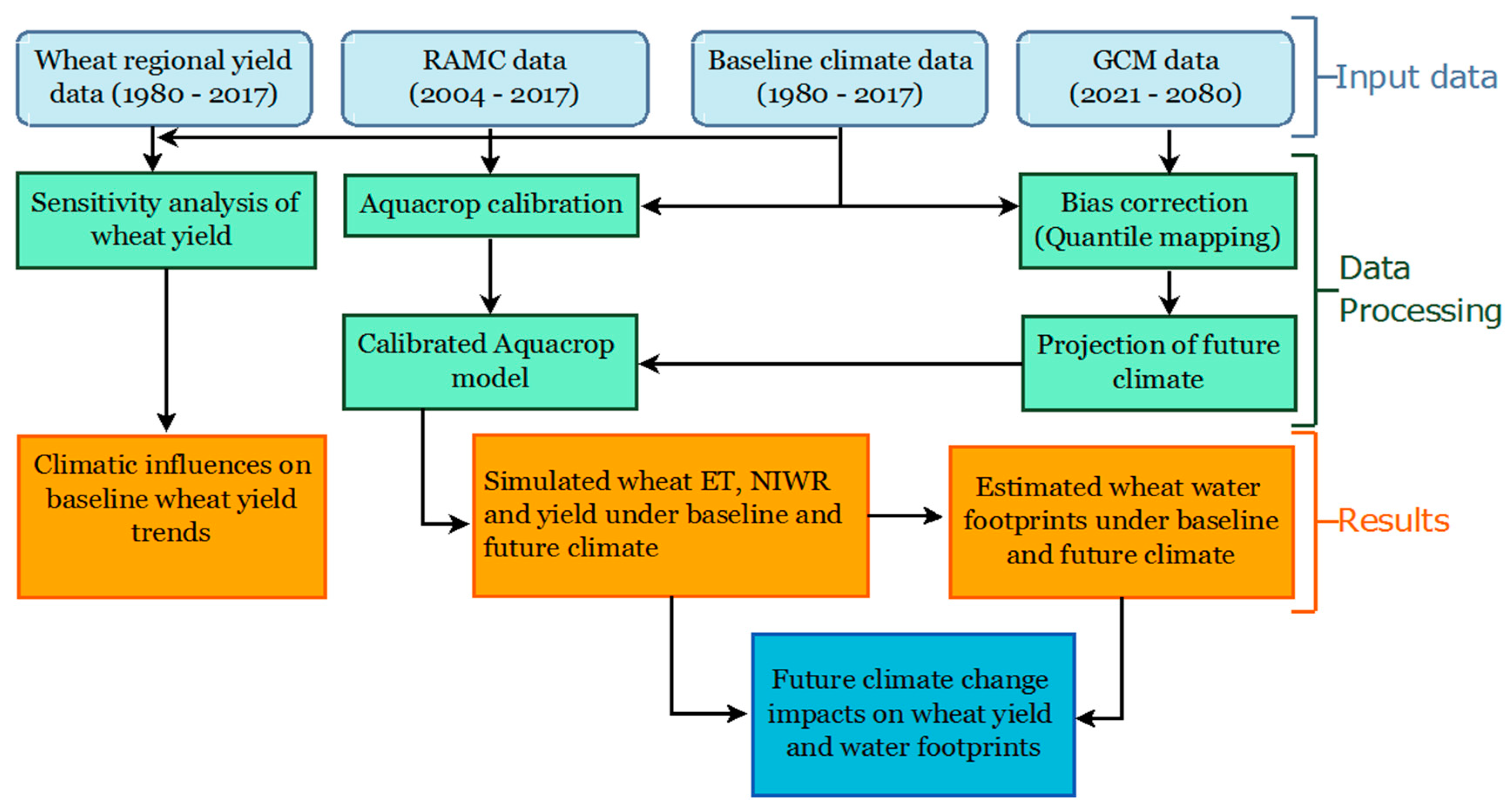
In Pakistan, Punjab province is the largest wheat producer in terms of cultivation area and yield (Figure 1a). This work focused on the district Faisalabad, Punjab, Pakistan. The Pakistan Meteorological Department (PMD) has established a regional agro-meteorological (RAMC) experimental site in this district to monitor the climate-induced influences on wheat yield variations (Figure 1b). The study district was selected due to the data available from the wheat field trials conducted at the RAMC site from 2004–2017 (annual crop reports available at http://namc.pmd.gov.pk/crop-reports.php). Winter and summer are the cropping seasons in the study area lasting from November–April and May–October, respectively. Wheat is the major winter crop and its sowing starts from middle of November to the end of December and harvesting lasts from mid-March to mid-April [14]. In this area, canal water is the primary irrigation water source as the poor-quality groundwater is not suitable for irrigated agriculture [26,27]. Arid to semi-arid climate dominates the agricultural lands and up to 70% of the annual rainfall occurs as monsoon rainfalls during the summer season. Average wheat seasonal maximum and minimum temperatures ranged from 23–27 °C and 3–8 °C, respectively; whereas wheat seasonal cumulative rainfall varied from 85–210 mm. Well-drained, sandy clay loam is the dominant soil texture in this area [28]. The methodology followed to achieve the study objectives is explained in Figure 2.

2.2. Sensitivity Analysis of Wheat Yield to Climate Variables

A sensitivity analysis was conducted to identify the most influential climate variable dictating the past wheat yield trends in the study area. PMD provided a daily climate data set comprising of maximum temperature (Tmax), minimum temperature (Tmin), solar radiation (Rn), relative humidity (RH), wind speed (u2) and rainfall (P) from 1980–2017. For the study district, the wheat production, cultivation area and yield (Y) data from 1980–2017 were also extracted from the Crop Reporting Service database, Government of Punjab, Pakistan (http://www.crs.agripunjab.gov.pk). Wheat seasonal (Nov–Apr) averaged Tmax and Tmin and seasonal cumulative Rn and P were included in the wheat Y sensitivity analysis. Change trends of wheat Y and the climate variable during the 1980–2017 were examined via simple linear regression with the year as an independent variable using the Equation (1):
V x = T x × Year + I x
where Vx represents the climate variable or wheat Y; Tx is the slope of the regression line representing the trend of the climate variable and Ix represents the intercept of the regression model. Statistical significance of the Tx was evaluated at 5% significance level.
Crop yields mostly exhibit increasing trends (TY) due to the improvements which occurred over time in the crop production and management practices and seed quality etc. [29]. The TY (kgha−1/year) comprised of a climate component (TY_Cli) which is only influenced by the climate factors and a management component (TY_Man) which defines the collective influences of crop production and management practices and other random factors (negligible). In order to establish climate-yield relationships, the TY_Cli and TY_Man must be isolated. The TY_Man can be removed from the TY by adopting de-trending techniques in which the inter-annual sensitivity of crop Y to climate variables is considered as a proxy for long-term climate change influences [30]. The first-difference method is a common de-trending approach which describes the absolute difference in Y or climate variables between two consecutive years [31]. We used the first-difference approach to de-trend the wheat TY during the 1980–2017 for the subsequent isolation of TY_Cli and TY_Man. The wheat TY was divided into the two components as follows [32,33]:
T Y = T Y _ Cli + T Y _ Man + e
where TY is actual wheat Y trend (kgha−1/year); TY_Cli, TY_Man and e represent the TY component influenced by the climate change, crop production and management practices and random factors (negligible), respectively. Wheat Y sensitivity to the climate variables was defined using the simple multiple linear regression. A relationship was established between the first-difference values of wheat Y and climate variables as follows [30,31,34]:
Δ Y = S Tmax × Δ T max + S Tmin × Δ T min + S Rn × Δ R n + S P × Δ P + ε
where ΔY, ΔTmax, ΔTmin, ΔTRn and ΔTP represent the first-difference values of the corresponding variables; STmax, STmin, SRn and SP are the coefficients of regression model representing the wheat Y sensitivity to the Tmax (kgha−1/°C), Tmin (kgha−1/°C), Rn (kgha−1/MJm−2) and P (kgha−1/mm), respectively; whereas, the ε is the intercept of the regression model. Finally, the TY_Cli was estimated using the following [31]:
T Y _ Cli = S Tmax × T Tmax + S Tmin × T Tmin + S Rn × T Rn + S P × T P
where the TTmax, TTmin, TRn and TP represent the trends of respective climate variable from the Equation (1) during the 1980–2017; while other parameters are same as defined in the Equation (3). The TY_Man was estimated indirectly using the Equation (2). Different climate variables could have varying relative contribution towards TY_Cli depending on their influences and change trends. For instance, the relative contribution of Tmax (RCTmax) towards wheat TY_Cli from 1980–2017 in the study district was estimated as [31]:
RC Tmax = S Tmax × T Tmax | S Tmax × T Tmax | + | S Tmin × T Tmin | + | S Rn × T Rn | + | S P × T P | × 100 %
where all the parameters in Equation (5) are same as defined in the Equations (1)–(4). Finally, the relative contribution of the four key climate variables was estimated using the Equation (5).

2.3. Future Climate Change Projection

In this study, future climate change projections were also included to predict their influences on wheat Y variations and water footprint. Outputs from nine global circulation models (GCM), listed in Table 1, forced under two representative concentration pathway scenarios (RCP 4.5 and 8.5) were employed to produce the future climate during two time slices: 2030s (2021–2050) and 2060s (2051–2080). The biases in the GCM-simulated and station-observed time series of Tmax, Tmin, Rn, RH, u2 and P during the baseline period of 1980–2010 were corrected through the quantile mapping (QM) approach.
QM approach tailors the cumulative distribution functions (CDF) of the GCM-simulated and station-observed time series of a specific climate variable during the baseline so that both the time series exhibit consistent means, variances and other statistical properties. Same empirical CDFs are then applied to the GCM-simulated future time series. More precisely, the misrepresented values in the GCM-simulated time series are replaced by the station-observed time series values given both the values have identical percentiles. Extensive discussion about the working principals, applications, and extensions of the QM and its performance comparison with other bias-correction approaches can be referenced from the literature [29,35,36,37]. In this work, a daily QM based bias-correction of the six major climate variables was conducted during the baseline and future time slices. CDFs of the daily Tmax, Tmin, Rn and P for the wheat season (Nov–Apr) during the baseline (1980–2010) before and after the application of QM are shown in Supplementary Figure S1. The bias-corrected outcomes of wheat seasonal Tmax, Tmin, Rn and P are also presented in Supplementary Figure S2.

2.4. Wheat Yield, Evapotranspiration and Net Irrigation Water Requirement

The water-driven Aquacrop model v5.0 developed by Food and Agriculture Organization (FAO) was used to simulate the soil water balance, wheat growth and Y process while maintaining robustness, simplicity and accuracy [38,39]. By incorporating the atmospheric evaporative demands via FAO Penman–Monteith reference crop evapotranspiration (ETo) and keeping track of incoming and outgoing water fluxes, the Aquacrop executes a daily water balance to determine actual crop evapotranspiration (ET); which in turn is further subdivided into transpiration (Tr) and evaporation (E) depending on the crop canopy cover and soil moisture status as follows [40,41,42]:
ET = E + Tr
E = K r × K e × ET o
Tr = K S × Kc Tr × ET o
where: Kr is the evaporation reduction coefficient, varying between 0 and 1, with the smaller value being indicative of insufficient water availability in the top 30 cm soil layer relative to the atmospheric evaporative demands; Ke is the soil evaporation coefficient, varying between 0 and 1, with smaller and larger values being proportional to and representatives of the fraction of soil surface covered by the canopy cover and exposed to the open atmosphere (no canopy cover), respectively; Ks is the water stress coefficient being equal to 1 and 0 at the field capacity and permanent wilting point, respectively; and the KcTr is the crop transpiration coefficient (0–1). Aquacrop transforms the seasonal cumulative Tr from the Equation (8) into the above-ground biomass (B) by multiplying it with the water productivity (WP*). The harvestable proportion of the B, which is the final crop yield (Y), is estimated from the product of B and crop-specific harvest index (HI) as follows:
B =   WP ×   Tr
Y = HI   × B
where: B and Y are tonha−1; WP* is kg per m2 per mm of water transpired and normalized for the atmospheric CO2 concentration and ETo, and HI is % [38,39,40,41,42].
In this study calibrated and validated Aquacrop input files, prepared using the experimental data collected from the RAMC Faisalabad site, were used to simulate the wheat ET, net irrigation water requirement (NIWR) and Y under the baseline and projected future climate. Detailed information about the experimental layout, wheat cultivars and soil type data used for Aquacrop calibration and performance evolution can be referenced from Ahmad, et al. [43]. The calibrated Aquacrop model was run in conjunction with bias-corrected climate change projections to simulate the future wheat NIWR, ET and Y. The sowing date was fixed as 20 November and the future NIWR was estimated by generating an automatic irrigation schedule in Aquacrop irrigation module with no water stress. Irrigation was set to trigger automatically when 50% of the total available water in the soil has been depleted to bring the root zone total soil moisture back to field capacity. Two simulation sets were run for modelling the wheat Y responses to atmospheric CO2 concentration: the first accounting for only the climate variations while keeping the CO2 concentrations at the baseline level of 390 ppm; and the second accounting for the combined effect of climate variations and elevated CO2 concentrations according to RCP 4.5 and 8.5 storylines [43].

2.5. Wheat Water Footprint

Frequently used [25,39,44] water footprint concept [18,19] was employed in this study to examine the wheat Y and water-usage (both P and NIWR) responses to projected future climate change. The term “water footprint” refers to the water consumption per unit production of a specific product. In the agriculture sector, total water footprint (WFtotal) designates the volumetric water consumption per unit of crop yield production (m3ton−1); and is further categorized as the WFgreen, WFblue and WFgrey. The WFgreen and WFblue represent the P and irrigation water consumption, respectively; whereas, the WFgrey accounts for the water usage for dissipating the pollutant loads generated from various material inputs such as fertilizer, pesticide and herbicide applications during the crop production process [20,21,22]. The WFblue and WFgreen of future wheat Y production in the study area were estimated as follows [20,21,45]:
WF blue = 10 × ET blue Y = 10 × NIWR Y
WF green = 10 × ET green Y = 10 × ( ET NIWR ) Y
where ETblue and ETgreen represent the P and irrigation water loss via evapotranspiration, respectively; factor 10 transforms the water depth (mm) into the water volume per area (m3ha−1); Y is the Aquacrop-simulated wheat yield (tonha−1) from the Equation (10). The degradative water usage for the wheat production-related pollutants dilution was estimated as follows [20,21,46]:
WF grey = α × AR c max × c nat × 1 Y
where AR is the chemical (fertilizer, pesticide and herbicide etc.) application rate (kg ha−1); α is the leaching-runoff fraction (%); and cmax and cnat are the maximum acceptable and natural concentration (mg L−1) of the considered pollutant in water, respectively.
Most WFgrey-related studies primarily focus on the pollution caused by Nitrogenous fertilizer application; which in turn governs the nitrate (NO3) leaching into the surface and sub-surface water bodies [3,22,23]. In this study, considering the Nitrogen AR for irrigated wheat production in Punjab [47]; the Equation (13) was employed to estimate only the Nitrogen related WFgrey by using the α = 10%; cmax = 10 mgL−1; and cnat = 0 [22,23,46]. Finally, the WFtotal were estimated as follows
W F total = W F green + W F blue + W F grey
The projected future wheat Y, NIWR and ET from the Equations (6)–(10) transformed the WFtotal into WFblue, WFgreen, and WFgrey components by using the Equations (11)–(14). For climate change impact assessment on wheat Y and WFs, baseline period was from 2004–2017 for which the field trial data were available from the RAMC Faisalabad site. For WFgrey estimations, the Nitrogen AR was assumed to remain unchanged in the future. Finally, variations in the 2030s- and 2060s-WFs from the respective baseline-averaged values, with and without the CO2 enrichment, were examined under the moderate (RCP 4.5) and extreme (RCP 8.5) emission scenarios.

3. Results and Discussion

3.1. Wheat Yield Sensitivity to Historic Climate

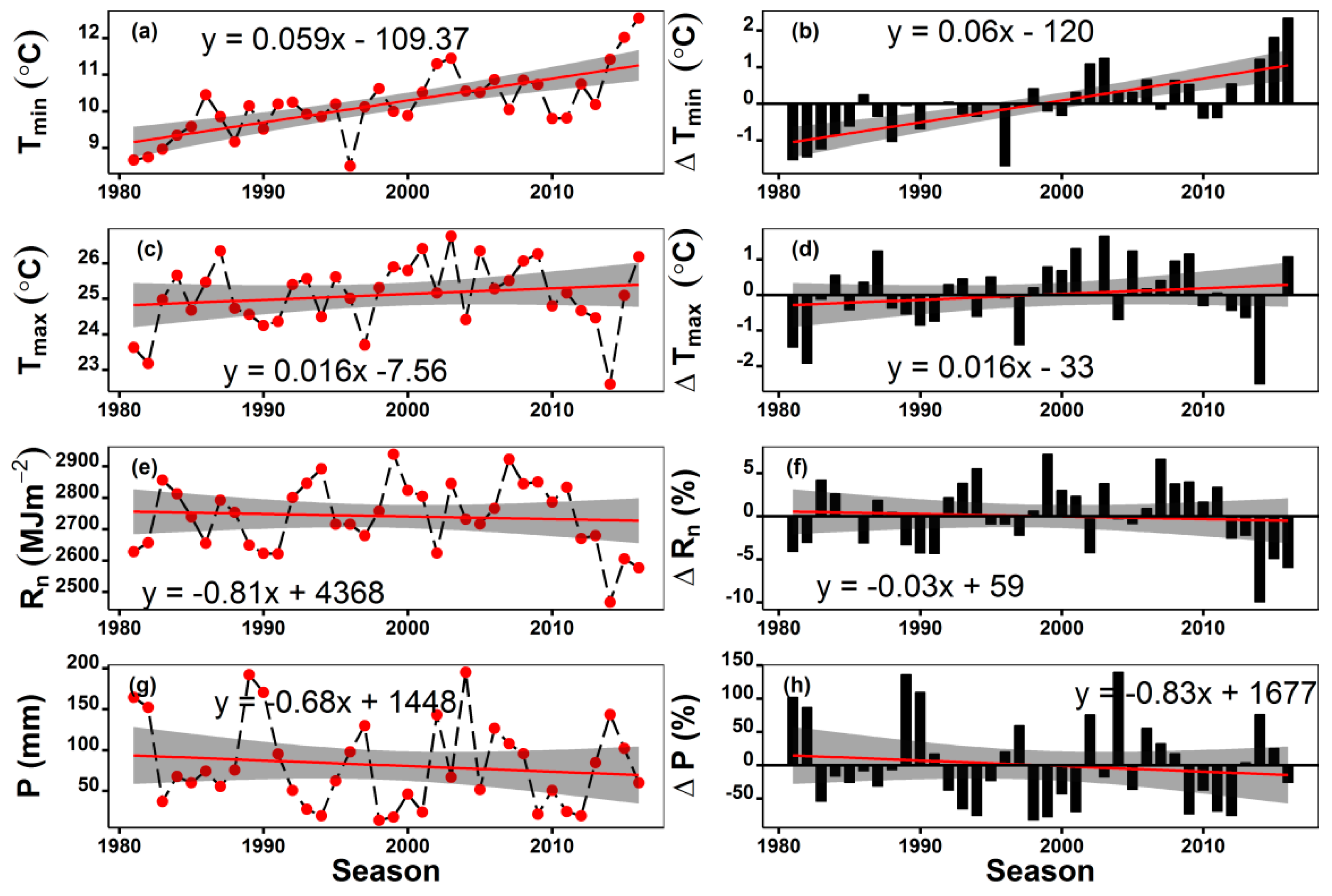
Inter-seasonal TTmax, TTmin, TRn and TP estimated from Equation (1) for the wheat season (Nov–Apr) from 1980–2017 are shown in Figure 3. TTmin was statistically significant and the TTmax, TRn and TP were statistically non-significant during the study period. TTmin and TTmax were increasing; whereas, the TRn and TP were declining over time (1980–2017). Both TTmin and TTmax were greater than anticipated global average temperature change of 0.13 °C decade−1 reported in the Intergovernmental Panel on Climate Change 5th Assessment Report (Figure 3a,c) [25,48]. In terms of magnitude and consistency, the TTmin was distinctly higher and prominent than those of the other climate variables. The respective change trends of Tmin, Tmax and P from their long-term average values were prominent after 2000; whereas, the negative Rn change trends were prominent during the last 5 years of the study period (Figure 3b,d,f,h).
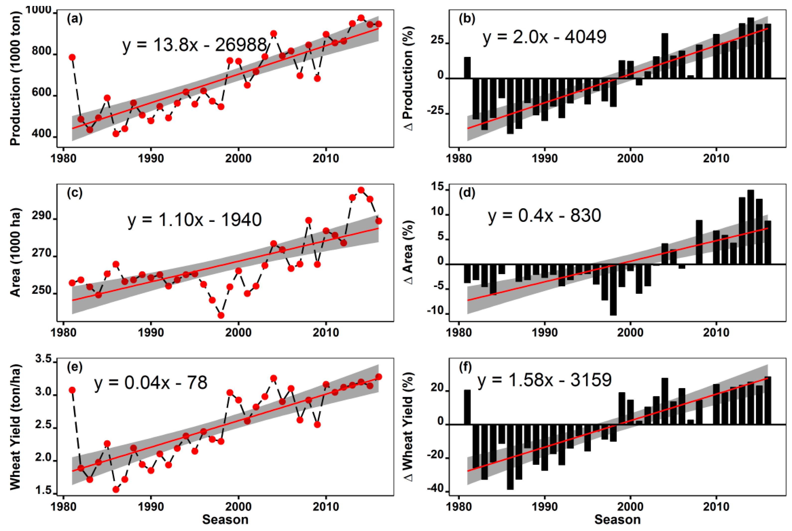
The wheat production, cultivation area and Y trends during the 1980–2017 are shown in Figure 4. Wheat TY was increasing significantly at the rate of 0.04 tonha−1/year or 36 kgha−1/year which seems to contradict the regional and global scale studies [11,12,49,50] constantly highlighting the warming-driven wheat Y decline risks. Generally, the long-term crop TY is positive because of improvements in crop production and management practices and seed quality; thus hiding the negative climate change influences [33].
In our study area, the wheat TY_Clim was estimated to be −7 kgha−1/year representing the wheat Y loss rate solely attributed to climate change in the study area. Despite the clearly evident harmful shifts in the thermal and rainfall regimes over course of the study period, the wheat TY was positive because of a gradual rise in cultivation area (Figure 4c) and improved production technologies. However, from 2010 and onwards the wheat Y change from its long-term average value was almost stagnant while the cultivation area was constantly rising (Figure 4c–f). This implied that TY_Cli has started to surpass the TY_Man and the current wheat cultivation and management practices would lag behind in sustaining the current wheat positive TY under future climate change trends.
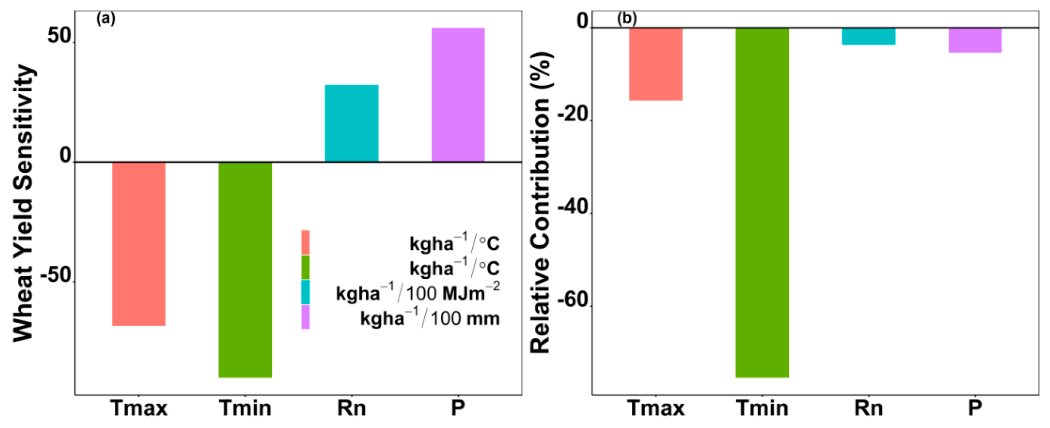
Wheat Y sensitivity to climate variables and their RC, depending on their respective influences and trends were estimated using the Equations (3)–(5) and the results are shown in Figure 5. STmin was highest followed by the STmax, SP and SRn; and wheat Y was negatively related to Tmin and Tmax and positively related to Rn and P, respectively. Compared to STmax and STmin, the SP was noticeably lower as wheat production in this area is primarily irrigated (Figure 5a). Contribution rate analysis showed that all the four climate variables had negative RC in an order according to their respective influences. Tmin was the major contributor because of its highest STmin and TTmin followed by the Tmax, P and Rn. Considering the difference between the STmin and STmax, the RCTmin and RCTmax differ greatly as the Tmax, despite being the second most influential climate variable, had a much lower TTmax than that of Tmin (Figure 5b). RCP and RCRn were also negative regardless of their positive relations with wheat Y as indicated by the SP and SRn in Figure 5a. Regardless of their mode of influence, the past trends of the four key climate variables were changing so as to contribute negatively towards wheat TY in the study area (Figure 5b).

3.2. Projected Future Climate Change

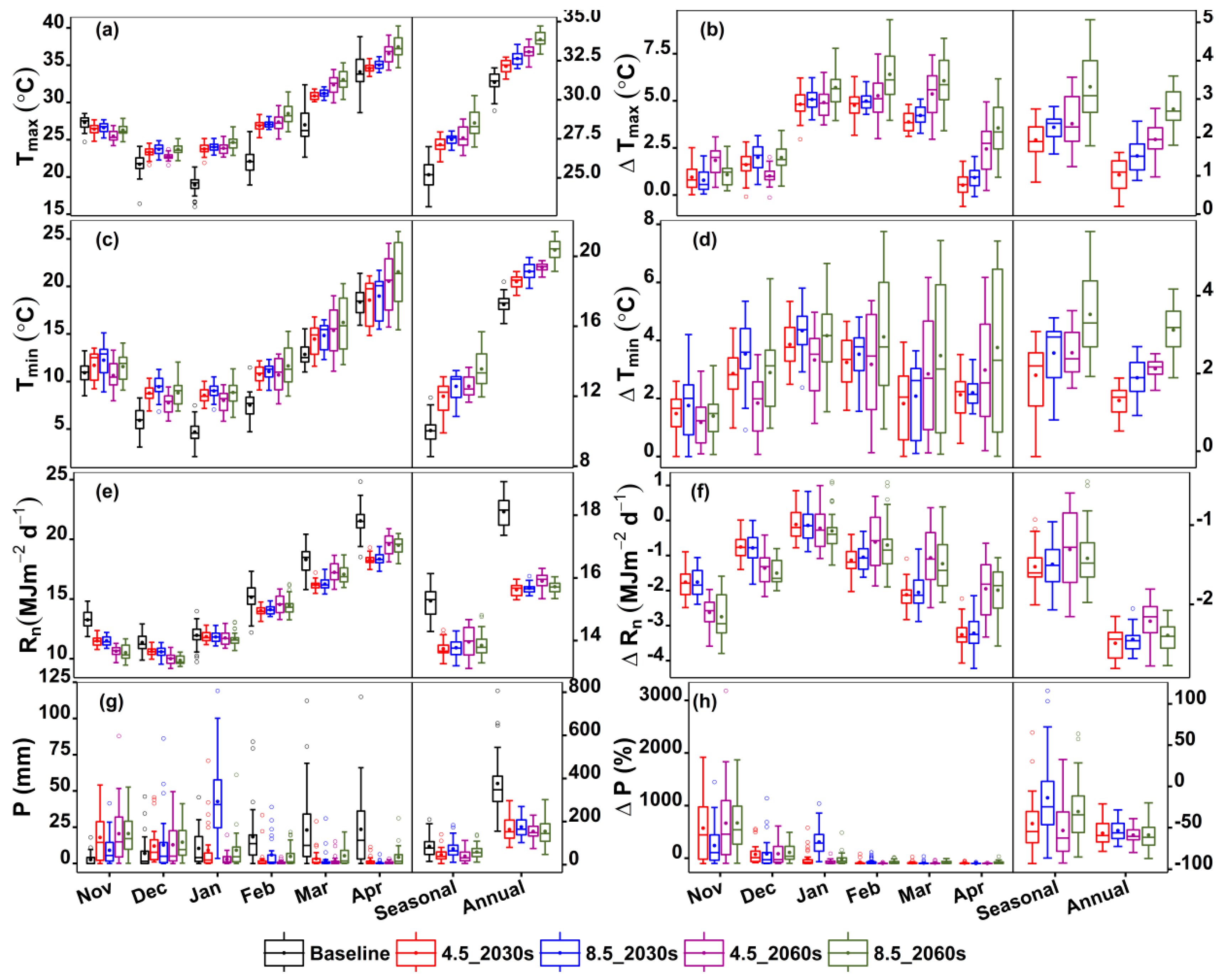
The projected changes in monthly, seasonal and annual Tmax, Tmin, Rn and P, after bias correction and averaged across nine GCMs, forced under RCP 4.5 and 8.5 during the baseline (1980–2010), the 2030s and 2060s are shown in Figure 6. Future climate of the study area in terms of Tmax, Tmin, Rn and P changed according to the past (1980–2017) climate change trends. Hence, the study area would undergo an intense and hotter thermal regime shift featuring prominent Tmin rise than Tmax accompanied by substantial seasonal cumulative Rn and P declines.
Anticipated climate warming (both Tmax and Tmin) was clearly evident at monthly, seasonal and annual scales irrespective of the GCM, RCP scenario (4.5 and 8.5) or future time slice (the 2030s and 2060s) (Figure 6a–d). The monthly Tmax and Tmin increased marginally during the first two months of the wheat season and then increased dramatically during the rest of the growing season. Change magnitude of the projected climate warming featured various noteworthy trends: Tmin > Tmax, wheat season > annual, RCP 8.5 > RCP 4.5 and 2060s > 2030s. The temperature change projections were supported by the last 30-year wheat seasonal average temperature inclines which were detected across most weather stations in Pakistan [13,14,51]. Trends and magnitudes of future climate warming projected in our study were also supported by the previous studies predicting the 21st-century climate of Pakistan [12,28,52].
Future wheat was particularly exposed to climate warming during the middle of the growing season from January to March. This could lead to a shortened grain filling duration but accelerating the gran filling rates which would not compensate for the probable Y reduction induced by shortened grain filling duration. Tmin is often associated with nighttime and prominent nighttime temperature increase could affect the spikelet fertility, grains per spike, grain size, and quality. Generally, wheat is particularly vulnerable to heat stress at anthesis and grain-filling stages [50]; for instance, the wheat Y in Pakistan is very sensitive to the mid-March higher temperature during grain filling stage [12].
Future monthly Rn also followed the temperature change trends but in a downward direction. Compared to the baseline, the future monthly Rn declined slightly during the first half; and greatly during the latter half of wheat season (Figure 6c) regardless of time slice or RCP. Contrary to the temperature, future Rn decline was prominent at the annual scale for both RCPs and time slices. For RCP 4.5, the seasonal- and annual-scale future Rn-decline was higher than its RCP 8.5 counterpart during both the time slices. Overall, the projected Rn decline with respect to baseline was: Annual > wheat season, RCP 4.5 > RCP 8.5 and 2030s > 2060s (Figure 6c,d).
The magnitude and direction of monthly, seasonal and annual P change in future varied greatly across GCMs. The future P declined or remained unchanged for most of the GCMs while rising P tendencies were envisaged by few GCMs. However, the GCM-ensemble wheat seasonal and annual P decreased with respect to the baseline (Figure 6g,h). Future monthly P increased from Nov–Jan; and then it declined drastically during the rest of the wheat season for both RCPs and time slices (Figure 6g,h). Hence, the future wheat would face severe P shortages along with excessive warming and Rn declines during the middle of the growing season which could decelerate the photosynthesis rates, increase the tiller infertility rate at Tmax = 36 °C and reduce the HI at Tmin >14 °C [12,49].
Similar to the Rn decline, future drying was also pronounced at the annual scale. Future wheat seasonal P decline was notably higher under RCP 4.5 than RCP 8.5; while the annual P decline remained almost the same under the two RCPs during both time slices. On average, 45–53% and 13–30% seasonal P decline; whereas 56%–60% and 53%–59% annual P decline was predicted by the end of the 21st century under the RCP 4.5 and 8.5, respectively.

3.3. Future Climate Change Impacts on Wheat ET and NIWR

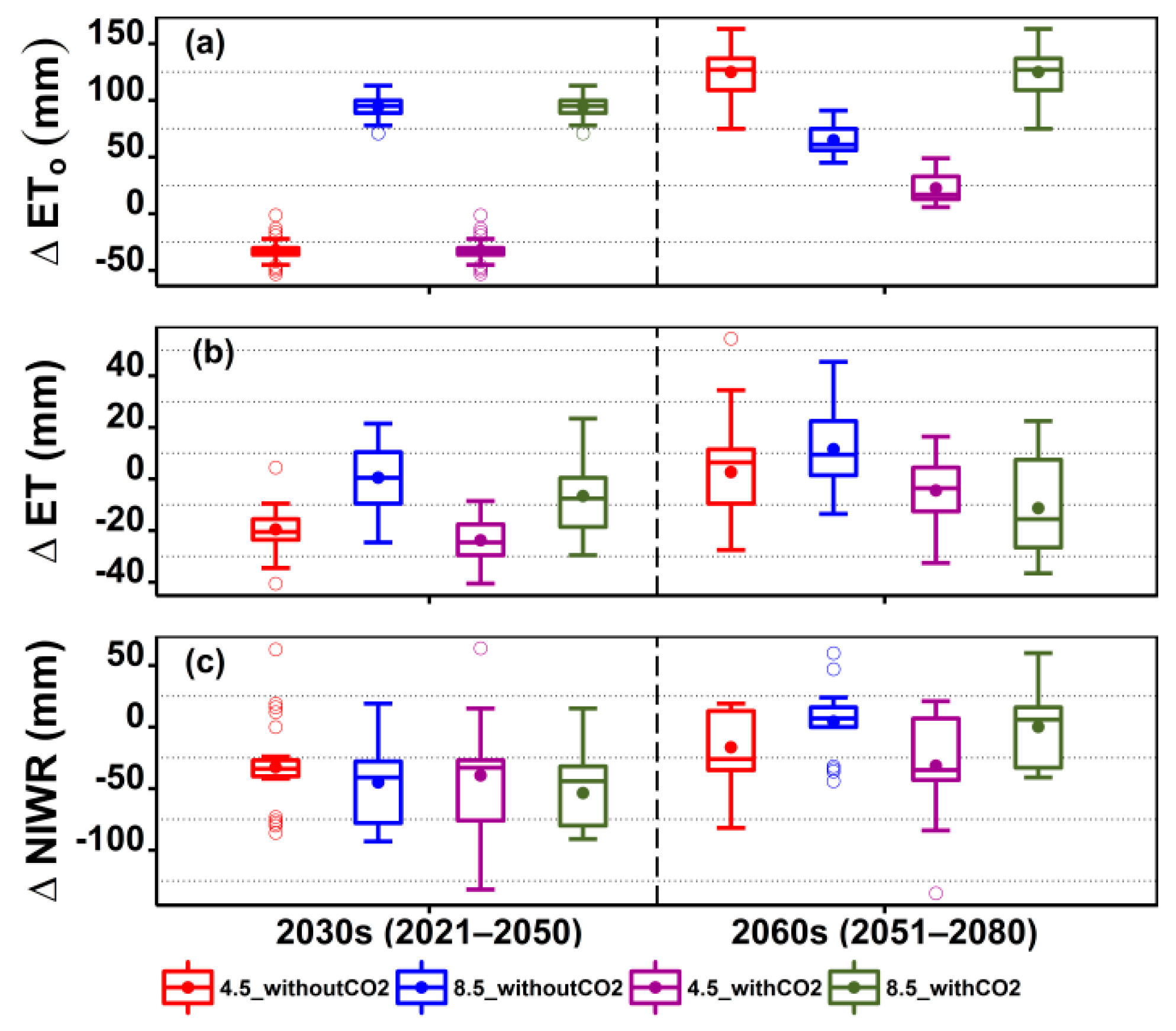
Wheat growing season length (GSL) recorded at the study site from 2004–2017 ranged between 116–145 days with an average of 130 days; while the seasonal cumulative growing degree days during this period ranged between 1545–1841 °C with an average of 1698 °C. From here on the term “baseline” refers to 2004–2017 period for which the wheat experimental data were available. Baseline average wheat seasonal cumulative ETo, ET and NIWR (simulated by Aquacrop) and P received during the GSL were 342, 285, 188, and 98 mm, respectively. Figure 7 presents the Aquacrop simulated GSL, ETo, ET, P and NIWR averaged during the baseline, the 2030s and 2060s. Projected wheat seasonal ETo, ET, and NIWR variations from the baseline during the 2030s and 2060s under the two RCPs with and without the CO2 enrichment are shown in Figure 8. The seasonal cumulative ETo, ET and NIWR for the wheat declined in the future which was odd as climate warming is often associated with accelerated ET rates and consequently higher NIWR [1,25]. The three parameters showed higher declining tendency during the 2030s particularly under RCP 4.5. Overall, the future wheat seasonal ETo, ET and NIWR had the minimum, medium and maximum declining likelihood, respectively, across the time slices or RCPs. Ambient temperature primarily controls the crop phenological progress and its increase often reduces the GSL due to rapid heat unit assimilations during crop growth stages [50]. Sultana, et al. [11] predicted a 12–14-day wheat-GSL shrinkage against future climate warming of up to 5 °C for the arid and semi-arid conditions of Pakistan. Bhatti, et al. [53] identified higher declining probabilities of ET and NIWR for the early maturing wheat in Punjab, Pakistan. In our study, future climate warming reduced the wheat-GSL by 10–12 days for RCP 4.5 and 13–20 days for RCP 8.5 by the end of 2080. This could explain the unexpected decline in the wheat seasonal cumulative ETo, ET and NIWR.
Because of moderate climate warming and the subsequent GSL shortening, the wheat seasonal cumulative ETo and ET declined only under RCP 4.5 during the 2030s; however, for rest of the cases, they increased because of intense climate warming despite a significant GSL shortening. During the 2030s, average ETo change was –32 mm and +95 mm; and during 2060s, it was +65 mm and +125 mm for RCP 4.5 and 8.5, respectively (Figure 8a). Future wheat ET change patterns were comparable with that of ETo but with slightly smaller change magnitudes. Contrary to conspicuously higher ETo change, mildly positive changes in future wheat ET were projected regardless of the RCP or time slice. During the 2030s, average ET change was −20 mm and +1 mm; and during 2060s, it was +3 mm and +12 mm for RCP 4.5 and 8.5, respectively (Figure 8b).
Difference between the crop ET and seasonal P determines the NIRW; which, in our study, showed the maximum declining likelihood compared to the ETo or ET. An average NIWR change of −32 mm and −45 mm during the 2030s; and −17 mm and +5 mm during the 2060s was shown for RCP 4.5 and 8.5, respectively (Figure 8c). The unexpectedly larger decline in 2030s-NIWR under RCP 8.5 was because of a positive seasonal-P change of +28 mm during this duration. The 2030s-P increased by 4% and 30%; and the 2060s-P decreased by 7% and 20% under RCP 4.5 and 8.5, respectively. It should be noted here that the future P-change trends discussed in Section 3.3 and shown as Figure 6h correspond to the general winter cropping season from Nov–Apr (180 days); whereas, the abovementioned future P-change trends correspond specifically to the wheat GSL (baseline average value = 130 days) as simulated by the Aquacrop.
Future wheat seasonal ETo, ET and NIWR were most likely to increase during the 2060s particularly under RCP 8.5. Furthermore, the difference between the 2030s- and 2060s-IQRs of the ETo, ET and NIWR change was larger for RCP 4.5 and smaller for RCP 8.5, respectively. Positive changes in wheat seasonal ETo, ET and NIWR were projected to begin at the start of the 2060s for the RCP 4.5; and during the middle of 2030s for RCP 8.5, respectively. Results suggested that frequent irrigations would be necessary to compensate for the warming-driven ET rates during a shortened growth span in the second half of the 21st century. CO2 enrichment did not induce any noticeable difference in the aforementioned ETo, ET and NIWR change patterns during the 2030s; however, during the 2060s, the CO2 enrichment partially contributed in limiting the warming-driven ETo, ET and NIWR increase tendencies regardless of RCP scenario (Figure 8a–c).
In addition to the probable contraction in wheat-GSL, the Rn decline could also be a leading cause of the drops in future ETo and ET identified in this study. Cloud cover, air pollutants and manmade aerosols affect the sunshine hours and Rn. An increased concentration of manmade aerosols and other air pollutants in the atmosphere can greatly reduce the incident Rn on a specific area [54]. This could explain the Rn decline detected in our study during the baseline and future time slices. Energy availability at the crop surface in the form of Rn plays a critical role in determining the water removal rate as ETo or ET [55]. ETo is highly sensitive to Rn and is directly related to Rn change patterns across various agro-ecological zones in Pakistan [14,56]. Based on a seasonal scale sensitivity analysis, we found that both the wheat ETo and ET were highly sensitive and positively related to Rn followed by Tmax, Tmin and P, respectively (results not shown here). This implied that future Rn decline could also limit the warming-driven ETo and ET increments. Our results showed that a combination of GSL and Rn decline would counteract the warming-driven ETo and ET increments during the 2030s; but it would not withhold these ETo and ET increments during the 2060s, ultimately resulting in higher NIWR during this duration. Similar conclusions were drawn by the recent studies from various parts of the world, in which the observed declines in ET and NIWR of various crops, despite a clear climate warming, were attributed either to GSL shortening and/or Rn declines [1,3,25,57].

3.4. Future Climate Change Impacts on Wheat Y and WFs

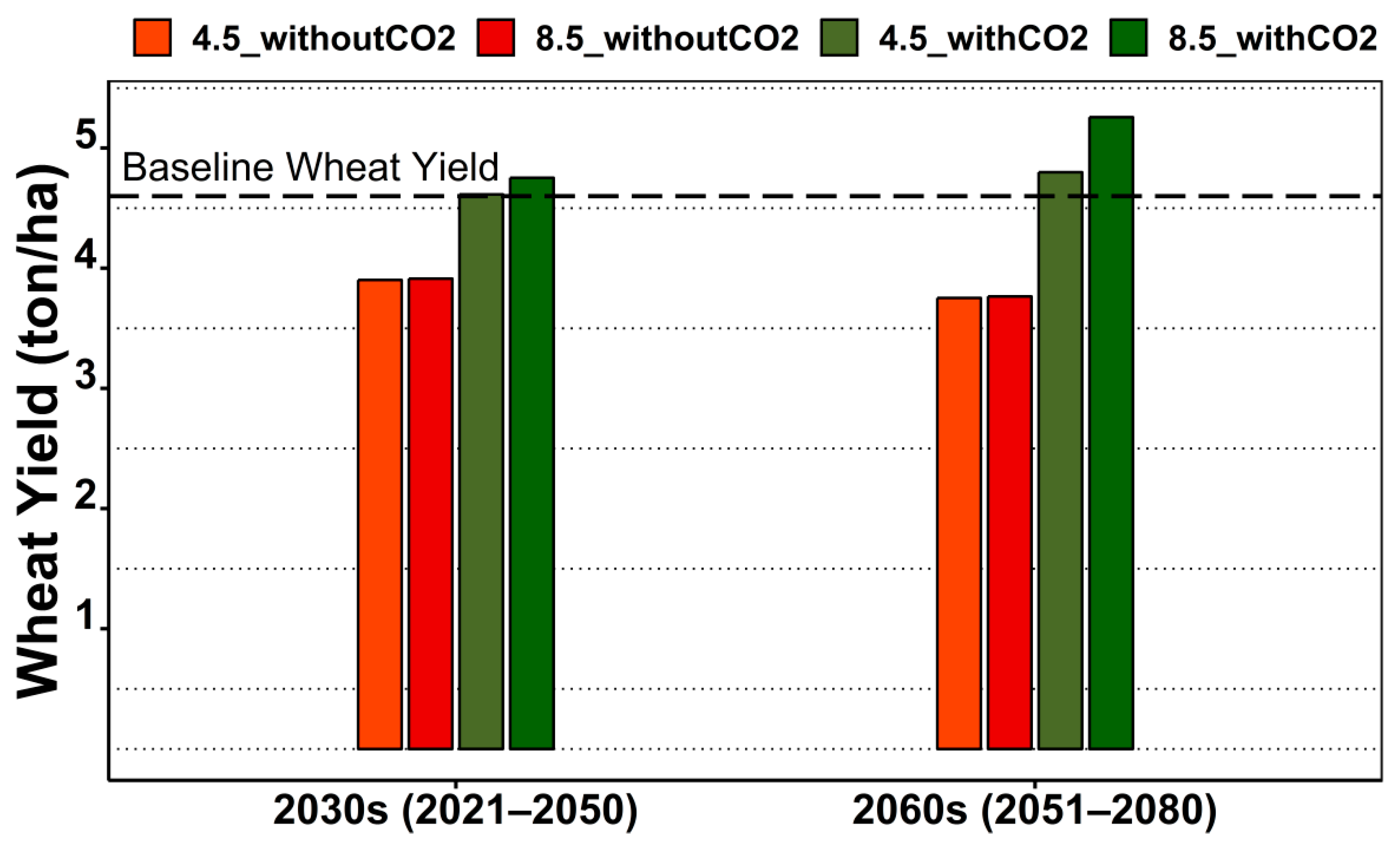
The average baseline wheat Y was 4.6 tonha−1. Comparison between average wheat Y simulated by the Aquacrop during the baseline, the 2030s and 2060s under the two RCPs with and without CO2 enrichment is shown in Figure 9. Moderate to severe wheat Y-declines at the baseline CO2 concentration of 390 ppm were detected during the 2030s and 2060s, respectively, regardless of RCPs. A potential rise in CO2 concentrations from 415–530 ppm (RCP 4.5) and from 420–750 ppm (RCP 8.5) partially and fully mitigated the wheat Y-declines prompted by future climate warming by end of the 2060s. Under RCP 8.5, despite the severe warming, 8–17% increments in future wheat Y were detected during the two time slices. Hence, by doubling the CO2 concentration up to 750 ppm under RCP 8.5, beneficial CO2 enrichment influences surpassed the negative climate warming impacts (Figure 9). These deductions were supported by findings of global-scale studies aimed at examining a composite climate change impact on future wheat Y resulting from the interplay between CO2 enrichment and climate warming [58,59].
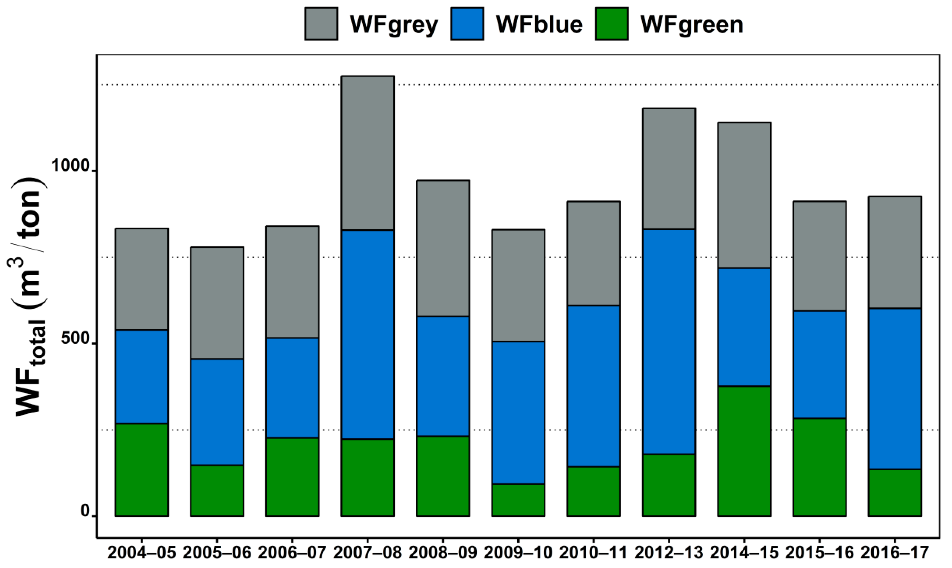
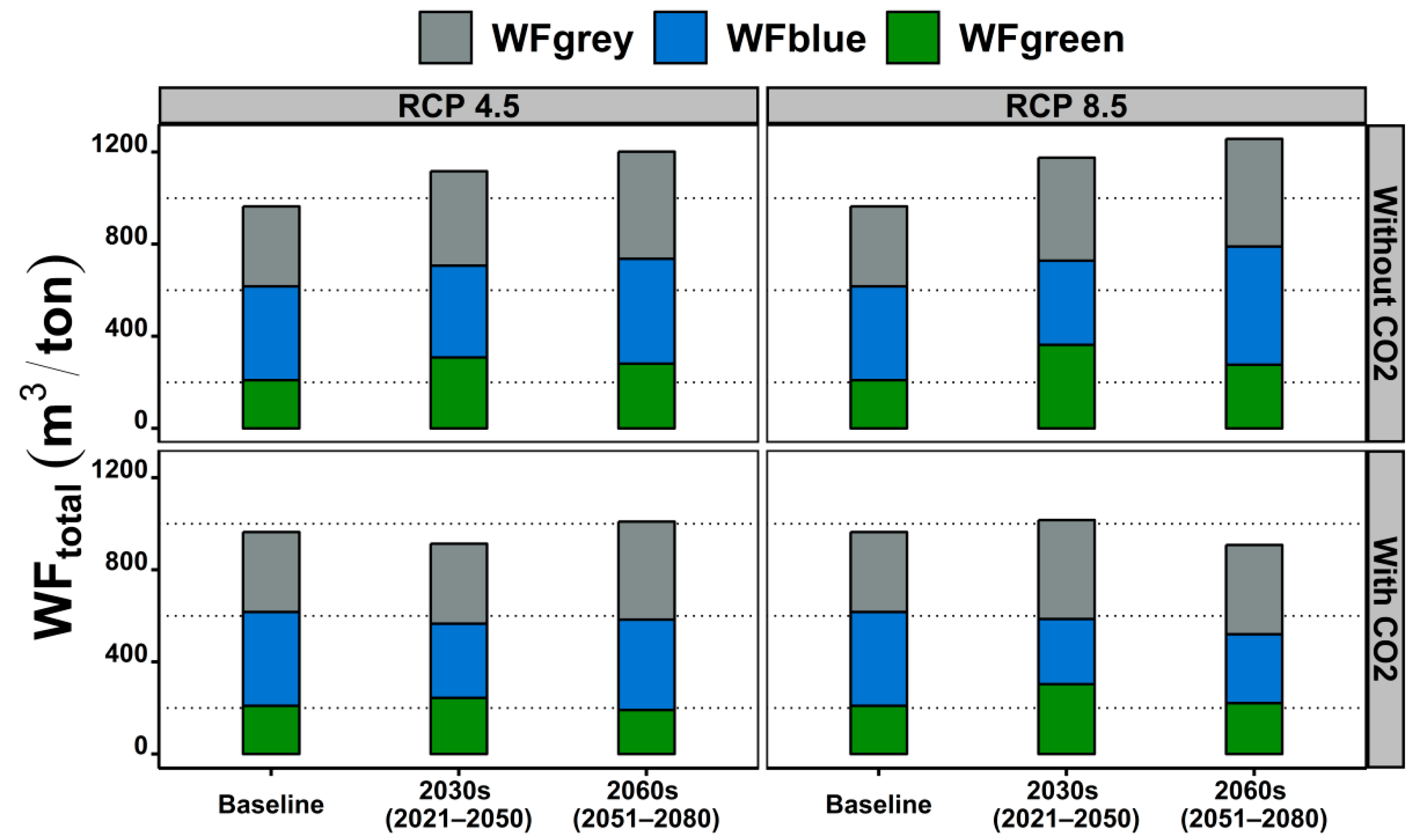
Wheat WFs for each season of the baseline period estimated using the Equations (11)–(14) are presented in Figure 10. The average WFgreen, WFblue, WFgrey and WFtotal during the baseline were 210, 407, 347, and 964 m3ton−1, respectively. Comparison between the average WFs during the baseline, the 2030s and 2060s are shown in Figure 11. Figure 12 shows the wheat WFs change from the baseline, averaged across nine GCMs, with and without the CO2 enrichment during the time slices and RCP scenarios.
Without the CO2 enrichment, the future WFs increased because of the wheat Y drop prompted by climate warming. Regarding the time slices, the 2060s-WFs increments were higher than those of the 2030s for both RCPs; whereas, for RCPs, the 8.5-WFs increments were higher than those of the 4.5 for both time slices except WFgreen which showed an opposite changing tendency. Wheat WFblue increased gradually to compensate for the green water scarcity originating from the projected drop in future P by the end of 2080. Under the enhanced CO2 concentrations, the wheat-WFs reduced negligibly during the 2030s and notably during the 2060s particularly under RCP 8.5 because of wheat-Y increments stimulated by CO2 enrichment (Figure 11).
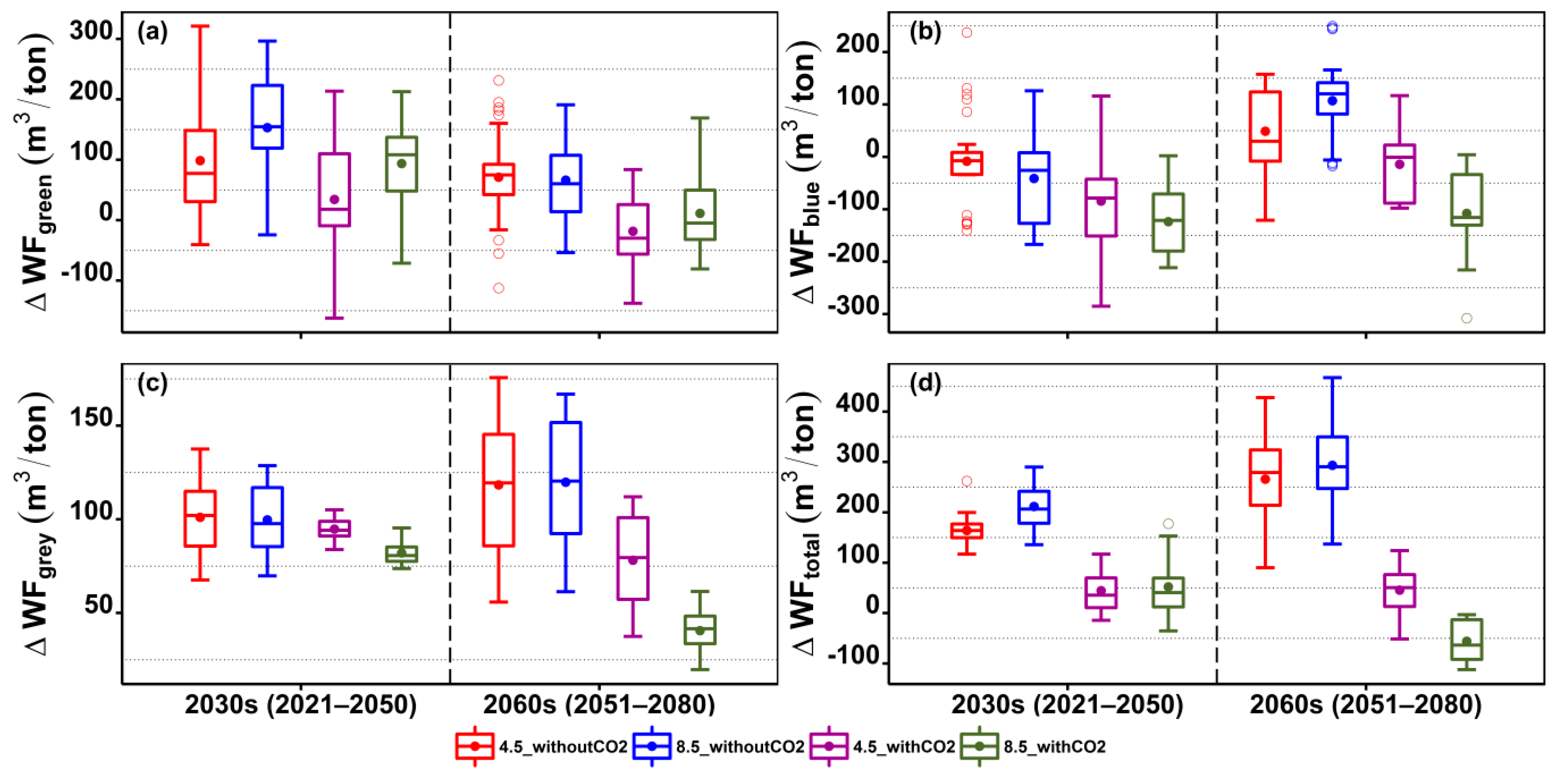
Despite having similar change trends, change magnitudes of the three WFs were not the same. Without CO2 enrichment, the 2030s-WFgreen increments were larger than the 2060s-WFgreen for both RCPs; indicating more green water availability per unit wheat Y or more Y production per unit of green water input. The 2030s duration featured moderate P increments which could explain the more green-water availability in this case. Because of higher wheat Y decline and a gradual rise in green water scarcity, the 2060s-WFgreen constantly declined irrespective of the RCPs or CO2 enrichment.
Contrary to the WFgreen, the rises in WFblue and WFgrey during the 2060s were higher than those of the 2030s because of the higher blue and grey water consumption per unit of the wheat Y production ultimately leading to higher WFtotal. WFblue and WFgrey increments during the 2030s were marginal because of a combination of moderate risks of climate warming, drying and wheat Y decline. During the 2060s, the warming-driven ET increments combined with a heightened risk of Y and P decline resulted in substantially higher blue and grey water consumption per unit of wheat Y production (Figure 12a–d). Among the three WFs, only the WFgrey exhibited a constantly increasing pattern irrespective of the time slice, RCP or atmospheric CO2 concentration (Figure 12c). Although the WFgrey declined because of wheat Y improvement caused by CO2 enrichment, its future changes remained consistently positive compared to the baseline. Results suggested that 50–150 m3ton−1 of extra greywater would be required to dissipate the pollutant load generated from Nitrogen application during future wheat production (Figure 12c).
The WFgreen, WFblue and WFtotal estimates produced in this study were slightly lower than the benchmark wheat WFs estimates at basin scale in Pakistan [22,23,60]. We calibrated the Aquacrop model using the field-scale wheat-trials data which were conducted under the optimum conditions such as without moisture, fertilizer or any other input restriction. Wheat Y from such trials could be very high compared to the farmer’s field and regional and basin-scale Y estimates. In our study, slightly higher wheat Y estimates were simulated by the Aquacrop, thus; producing slightly lower WFs values. Moreover, we only consider the optimum NIWR for WFblue estimation without considering the conveyance losses or excessive field-scale irrigation water applications by the farmers which are an integral part of WF-estimation framework at a larger spatial scale. However, replacing the Aquacrop simulated wheat Y with regional statistical Y would produce similar WFs outcomes according to the benchmark values provided in the aforementioned studies. This work mainly examines the wheat-WFs change-patterns in place of their absolute values to approximate the future climate change impacts on wheat water management in the study area. Based on various climate change probabilities examined in this study, the most unlikely and extreme scenario of RCP 8.5 exhibited the prospects of CO2 enrichment convincingly nullifying the future warming during the 2nd half of the 21st century. For the rest of the cases, the mitigation potential of CO2 enrichment against future climate warming remained limited. This implied that CO2 enrichment could partially compensate for the detrimental warming impacts on the future wheat Y and WFs in semi-arid regions of Punjab, Pakistan.

4. Conclusions

Wheat yield sensitivity to past climate change trends and its variability under projected future climate change was quantified for semi-arid conditions of Punjab, Pakistan. Identical past and projected future climate change trends were shown with wheat yield being inversely related to growing seasonal averaged Tmin and Tmax, and directly related to growing seasonal cumulative Rn and P. Tmin was the principal climate driver contributing to the past and future wheat yield trends followed by the Tmax, P and Rn. Warming-driven accelerated crop development process enhanced the yield failure risks in the future early-maturing wheat crop; however, the CO2 enrichment partially compensated the detrimental warming impacts on wheat yield. Wheat ET and NIWR declined due to the influence of both decrease of growing season length and Rn for the first half of 21st-century, and this trend reversed during the second half of 21st-century. Rampant green water scarcity exerted extra pressure of blue water resources, particularly during 2nd-time slices while extra greywater was required to dissipate the pollutant load generated from Nitrogen application. Devising irrigation schedules to maximize the green water consumption could alleviate the anticipated stresses on blue water resources. Adaptation of field management practices to maintain and improve soil organic matter and water holding capacities can also reduce the grey and blue water consumptions by facilitating the nutrient and blue water availability to the crop. Development of suitable crop cultivars having better heat tolerance and Rn interception capacity could be a long-term and reliable solution for maintaining wheat yields under future climate warming.

Supplementary Materials

The following are available online at https://www.mdpi.com/2073-4395/9/11/744/s1, Figure S1: Comparison between cumulative distribution functions (CDF) of daily (a) Tmax, (b) Tmin, (c) solar radiation (Rn) and (d) rainfall (P) for wheat season (Nov–Apr) during the baseline (1980–2010) period. Each red and green line represents an ensemble-output of nine GCMs before and after bias correction, Figure S2: Bias correction of wheat seasonal-average Tmax, Tmin, solar radiation (Rn) and seasonal cumulative rainfall (P) during the baseline (1980–2010) period. The box represents the interquartile range (IQR), the whiskers extend up to 1.5 times the IQR, the dot and horizontal line inside the box represent mean and median, respectively, and outliers are shown as hollow dots outside the box

Author Contributions

Conceptualization, M.J.A. and K.-S.C.; methodology, M.J.A. and K.-S.C.; software, M.J.A., G.-H.C and S.-H.K; validation, G.-H.C and S.-H.K.; formal analysis, M.J.A.; investigation, G.-H.C and S.-H.K.; resources, M.J.A., K.-S.C; data curation, G.-H.C and K.-S.C; writing—original draft preparation, M.J.A.; writing—review and editing, M.J.A., K.-S.C. visualization, M.J.A., G.-H.C and S.-H.K.; supervision, K.-S.C.

Funding

This research received no external funding.

Conflicts of Interest

The authors declare no conflict of interest.

References

  1. Sun, S.K.; Li, C.; Wu, P.T.; Zhao, X.N.; Wang, Y.B. Evaluation of agricultural water demand under future climate change scenarios in the Loess Plateau of Northern Shaanxi, China. Ecol. Indic. 2018, 84, 811–819. [Google Scholar] [CrossRef]
  2. Sun, S.; Wu, P.; Wang, Y.; Zhao, X.; Liu, J.; Zhang, X. The impacts of interannual climate variability and agricultural inputs on water footprint of crop production in an irrigation district of China. Sci. Total Environ. 2013, 444, 498–507. [Google Scholar] [CrossRef] [PubMed]
  3. Shrestha, S.; Chapagain, R.; Babel, M.S. Quantifying the impact of climate change on crop yield and water footprint of rice in the Nam Oon Irrigation Project, Thailand. Sci. Total Environ. 2017, 599–600, 689–699. [Google Scholar] [CrossRef] [PubMed]
  4. Khan, M.A.; Khan, J.A.; Ali, Z.; Ahmad, I.; Ahmad, M.N. The challenge of climate change and policy response in Pakistan. Environ. Earth Sci. 2016, 75, 1–16. [Google Scholar] [CrossRef]
  5. Abid, M.; Schilling, J.; Scheffran, J.; Zulfiqar, F. Climate change vulnerability, adaptation and risk perceptions at farm level in Punjab, Pakistan. Sci. Total Environ. 2016, 547, 447–460. [Google Scholar] [CrossRef] [PubMed]
  6. Archer, D.R.; Forsythe, N.; Fowler, H.J.; Shah, S.M. Sustainability of water resources management in the Indus Basin under changing climatic and socio economic conditions. Hydrol. Earth Syst. Sci. 2010, 14, 1669–1680. [Google Scholar] [CrossRef]
  7. Bhatti, A.M.; Suttinon, P.; Nasu, S. Agriculture water demand management in Pakistan: A review and perspective. Internet J. Soc. Soc. Manag. Syst. 2009, 9, 1–7. [Google Scholar]
  8. Arshad, M.; Amjath-Babu, T.; Krupnik, T.J.; Aravindakshan, S.; Abbas, A.; Kächele, H.; Müller, K. Climate variability and yield risk in South Asia’s rice-wheat systems: Emerging evidence from Pakistan. Paddy Water Environ. 2017, 15, 249–261. [Google Scholar] [CrossRef]
  9. Kirby, M.; Ahmad, M.-u.-D.; Mainuddin, M.; Khaliq, T.; Cheema, M.J.M. Agricultural production, water use and food availability in Pakistan: Historical trends, and projections to 2050. Agric. Water Manag. 2017, 179, 34–46. [Google Scholar] [CrossRef]
  10. Khaliq, T.; Gaydon, D.S.; Ahmad, M.-u.-D.; Cheema, M.J.M.; Gull, U. Analyzing crop yield gaps and their causes using cropping systems modelling—A case study of the Punjab rice-wheat system, Pakistan. Field Crop. Res. 2019, 232, 119–130. [Google Scholar] [CrossRef]
  11. Sultana, H.; Ali, N.; Iqbal, M.M.; Khan, A.M. Vulnerability and adaptability of wheat production in different climatic zones of Pakistan under climate change scenarios. Clim. Chang. 2009, 94, 123–142. [Google Scholar] [CrossRef]
  12. Hussain, J.; Khaliq, T.; Ahmad, A.; Akhter, J.; Asseng, S. Wheat Responses to Climate Change and Its Adaptations: A Focus on Arid and Semi-arid Environment. Int. J. Environ. Res. 2018, 12, 117–126. [Google Scholar] [CrossRef]
  13. Iqbal, M.A.; Penas, A.; Cano-Ortiz, A.; Kersebaum, K.; Herrero, L.; del Río, S. Analysis of recent changes in maximum and minimum temperatures in Pakistan. Atmos. Res. 2016, 168, 234–249. [Google Scholar] [CrossRef]
  14. Ahmad, M.J.; Choi, K.S. Influence of climate variables on FAO Penman–Monteith reference evapotranspiration in the Upper Chenab Canal command area of Pakistan. Paddy Water Environ. 2018, 16, 425–438. [Google Scholar] [CrossRef]
  15. Laghari, A.N.; Vanham, D.; Rauch, W. The Indus basin in the framework of current and future water resources management. Hydrol. Earth Syst. Sci. 2012, 16, 1063–1083. [Google Scholar] [CrossRef]
  16. Rasul, G.; Mahmood, A.; Sadiq, A.; Khan, S. Vulnerability of Indus delta to climate change in Pakistan. Pak. J. Meteorol. 2012, 8, 89–107. [Google Scholar]
  17. Rasul, G.; Chaudhry, Q.; Mahmood, A.; Hyder, K. Effect of temperature rise on crop growth and productivity. Pak. J. Meteorol. 2011, 8, 53–62. [Google Scholar]
  18. Hoekstra, A.Y. Green-blue water accounting in a soil water balance. Adv. Water Resour. 2019, 129, 112–117. [Google Scholar] [CrossRef]
  19. Hoekstra, A.Y. Water Footprint Assessment: Evolvement of a New Research Field. Water Resour. Manag. 2017, 31, 3061–3081. [Google Scholar] [CrossRef]
  20. Hoekstra, A.Y.; Chapagain, A.K.; Aldaya, M.M.; Mekonnen, M.M. The Water Footprint Assessment Manual: Setting the Global Standard; Earthscan: Washington, DC, USA, 2011. [Google Scholar]
  21. Hoekstra, A.Y.; Chapagain, A.K.; Aldaya, M.M.; Mekonnen, M.M. Water Footprint Manual: State of the Art 2009; Water Footprint Network: Enschede, The Netherlands, 2009. [Google Scholar]
  22. Mekonnen, M.M.; Hoekstra, A.Y. The green, blue and grey water footprint of crops and derived crop products. Hydrol. Earth Syst. Sci. 2011, 15, 1577–1600. [Google Scholar] [CrossRef]
  23. Mekonnen, M.M.; Hoekstra, A.Y. A global and high-resolution assessment of the green, blue and grey water footprint of wheat. Hydrol. Earth Syst. Sci. 2010, 14, 1259–1276. [Google Scholar] [CrossRef]
  24. Velpuri, N.M.; Senay, G.B. Partitioning evapotranspiration into green and blue water sources in the conterminous United States. Sci. Rep. 2017, 7, 6191. [Google Scholar] [CrossRef] [PubMed]
  25. Zhao, Y.; Ding, D.; Si, B.; Zhang, Z.; Hu, W.; Schoenau, J. Temporal variability of water footprint for cereal production and its controls in Saskatchewan, Canada. Sci. Total Environ. 2019, 660, 1306–1316. [Google Scholar] [CrossRef] [PubMed]
  26. Usman, M.; Liedl, R.; Shahid, M.A. Managing Irrigation Water by Yield and Water Productivity Assessment of a Rice-Wheat System Using Remote Sensing. J. Irrig. Drain. Eng. 2014, 140, 401–422. [Google Scholar] [CrossRef]
  27. Usman, M.; Liedl, R.; Kavousi, A. Estimation of distributed seasonal net recharge by modern satellite data in irrigated agricultural regions of Pakistan. Environ. Earth Sci. 2015, 74, 1463–1486. [Google Scholar] [CrossRef]
  28. Iqbal, M.A.; Eitzinger, J.; Formayer, H.; Hassan, A.; Heng, L.K. A simulation study for assessing yield optimization and potential for water reduction for summer-sown maize under different climate change scenarios. J. Agric. Sci. 2011, 149, 129–143. [Google Scholar] [CrossRef]
  29. Miao, C.; Su, L.; Sun, Q.; Duan, Q. A nonstationary bias-correction technique to remove bias in GCM simulations. J. Geophys. Res. Atmos. 2016, 121, 5718–5735. [Google Scholar] [CrossRef]
  30. Kukal, M.S.; Irmak, S. Climate-Driven Crop Yield and Yield Variability and Climate Change Impacts on the U.S. Great Plains Agricultural Production. Sci. Rep. 2018, 8, 3450. [Google Scholar] [CrossRef] [PubMed]
  31. Liu, Y.; Chen, Q.; Ge, Q.; Dai, J.; Qin, Y.; Dai, L.; Zou, X.; Chen, J. Modelling the impacts of climate change and crop management on phenological trends of spring and winter wheat in China. Agric. For. Meteorol. 2018, 248, 518–526. [Google Scholar] [CrossRef]
  32. Dong, Z.; Pan, Z.; He, Q.; Wang, J.; Huang, L.; Pan, Y.; Han, G.; Xue, X.; Chen, Y. Vulnerability assessment of spring wheat production to climate change in the Inner Mongolia region of China. Ecol. Indic. 2018, 85, 67–78. [Google Scholar] [CrossRef]
  33. Troy, T.J.; Kipgen, C.; Pal, I. The impact of climate extremes and irrigation on US crop yields. Environ. Res. Lett. 2015, 10, 054013. [Google Scholar] [CrossRef]
  34. Adisa, O.M.; Botai, C.M.; Botai, J.O.; Hassen, A.; Darkey, D.; Tesfamariam, E.; Adisa, A.F.; Adeola, A.M.; Ncongwane, K.P. Analysis of agro-climatic parameters and their influence on maize production in South Africa. Theor. Appl. Climatol. 2018, 134, 991–1004. [Google Scholar] [CrossRef]
  35. Sippel, S.; Otto, F.E.L.; Forkel, M.; Allen, M.R.; Guillod, B.P.; Heimann, M.; Reichstein, M.; Seneviratne, S.I.; Thonicke, K.; Mahecha, M.D. A novel bias correction methodology for climate impact simulations. Earth Syst. Dyn. 2016, 7, 71–88. [Google Scholar] [CrossRef]
  36. Rockel, B. The Regional Downscaling Approach: A Brief History and Recent Advances. Curr. Clim. Chang. Rep. 2015, 1, 22–29. [Google Scholar] [CrossRef]
  37. Eum, H.-I.; Cannon, A.J. Intercomparison of projected changes in climate extremes for South Korea: Application of trend preserving statistical downscaling methods to the CMIP5 ensemble. Int. J. Climatol. 2017, 37, 3381–3397. [Google Scholar] [CrossRef]
  38. Steduto, P.; Hsiao, T.C.; Raes, D.; Fereres, E. AquaCrop—The FAO crop model to simulate yield response to water: I. Concepts and underlying principles. Agron. J. 2009, 101, 426–437. [Google Scholar] [CrossRef] [Green Version]
  39. Chukalla, A.; Krol, M.; Hoekstra, A. Green and blue water footprint reduction in irrigated agriculture: Effect of irrigation techniques, irrigation strategies and mulching. Hydrol. Earth Syst. Sci. 2015, 19, 4877–4891. [Google Scholar] [CrossRef] [Green Version]
  40. Raes, D.; Steduto, P.; Hsiao, T.C.; Fereres, E. Aquacrop the FAO crop model to simulate yield response to water: II. Main algorithms and software description. Agron. J. 2009, 101, 438–447. [Google Scholar] [CrossRef] [Green Version]
  41. Hsiao, T.C.; Heng, L.; Steduto, P.; Rojas-Lara, B.; Raes, D.; Fereres, E. AquaCrop—The FAO crop model to simulate yield response to water: III. Parameterization and testing for maize. Agron. J. 2009, 101, 448–459. [Google Scholar] [CrossRef]
  42. Heng, L.K.; Hsiao, T.; Evett, S.; Howell, T.; Steduto, P. Validating the FAO AquaCrop model for irrigated and water deficient field maize. Agron. J. 2009, 101, 488–498. [Google Scholar] [CrossRef] [Green Version]
  43. Ahmad, M.J.; Iqbal, M.A.; Choi, K.S. Climate-driven constraints in sustaining future wheat yield and water productivity. Agric. Water Manag. 2019. (First revision submitted on 21 October 2019). [Google Scholar]
  44. Xinchun, C.; Mengyang, W.; Rui, S.; La, Z.; Dan, C.; Guangcheng, S.; Xiangping, G.; Weiguang, W.; Shuhai, T. Water footprint assessment for crop production based on field measurements: A case study of irrigated paddy rice in East China. Sci. Total Environ. 2018, 610–611, 84–93. [Google Scholar] [CrossRef] [PubMed]
  45. Zhang, Y.; Huang, K.; Ridoutt, B.G.; Yu, Y. Comparing volumetric and impact-oriented water footprint indicators: Case study of agricultural production in Lake Dianchi Basin, China. Ecol. Indic. 2018, 87, 14–21. [Google Scholar] [CrossRef]
  46. Franke, N.; Boyacioglu, H.; Hoekstra, A. Grey Water Footprint Accounting: Tier 1 Supporting Guidelines; Value of Water Research Report Series No. 65; UNESCO-IHE: Delft, The Netherlands, 2013. [Google Scholar]
  47. Fertilizer Use by Crop in Pakistan; Food and Agriculture Organization of the United Nations: Rome, Italy, 2004.
  48. Stocker, T.F.; Qin, D.; Plattner, G.-K.; Tignor, M.; Allen, S.K.; Boschung, J.; Nauels, A.; Xia, Y.; Bex, V.; Midgley, P.M. The Physical Science Basis. Contribution of Working Group I to the Fifth Assessment Report of the Intergovernmental Panel on Climate Change; Cambridge University Press: Cambridge, UK; New York, NY, USA, 2013; p. 1535. [Google Scholar]
  49. Asseng, S.; Foster, I.A.N.; Turner, N.C. The impact of temperature variability on wheat yields. Glob. Chang. Biol. 2011, 17, 997–1012. [Google Scholar] [CrossRef]
  50. Asseng, S.; Ewert, F.; Martre, P.; Rotter, R.P.; Lobell, D.B.; Cammarano, D.; Kimball, B.A.; Ottman, M.J.; Wall, G.W.; White, J.W.; et al. Rising temperatures reduce global wheat production. Nat. Clim. Chang. 2015, 5, 143–147. [Google Scholar] [CrossRef]
  51. Ahmad, W.; Fatima, A.; Awan, U.K.; Anwar, A. Analysis of long term meteorological trends in the middle and lower Indus Basin of Pakistan: A non-parametric statistical approach. Glob. Planet. Chang. 2014, 122, 282–291. [Google Scholar] [CrossRef]
  52. Islam, S.u.; Rehman, N.; Sheikh, M.M. Future change in the frequency of warm and cold spells over Pakistan simulated by the PRECIS regional climate model. Clim. Chang. 2009, 94, 35–45. [Google Scholar] [CrossRef]
  53. Bhatti, M.T.; Balkhair, K.S.; Masood, A.; Sarwar, S. Optimized shifts in sowing times of field crops to the projected climate changes in an agro-climatic zone of Pakistan. Exp. Agric. 2016, 1–13. [Google Scholar] [CrossRef]
  54. Liu, H.; Li, Y.; Josef, T.; Zhang, R.; Huang, G. Quantitative estimation of climate change effects on potential evapotranspiration in Beijing during 1951–2010. J. Geogr. Sci. 2014, 24, 93–112. [Google Scholar] [CrossRef]
  55. Allen, R.G.; Pereira, L.S.; Howell, T.A.; Jensen, M.E. Evapotranspiration information reporting: I. Factors governing measurement accuracy. Agric. Water Manag. 2011, 98, 899–920. [Google Scholar] [CrossRef] [Green Version]
  56. Adnan, S.; Ullah, K.; Khan, A.H.; Gao, S. Meteorological impacts on evapotranspiration in different climatic zones of Pakistan. J. Arid Land 2017, 9, 938–952. [Google Scholar] [CrossRef] [Green Version]
  57. Acharjee, T.K.; Halsema, G.v.; Ludwig, F.; Hellegers, P. Declining trends of water requirements of dry season Boro rice in the north-west Bangladesh. Agric. Water Manag. 2017, 180, 148–159. [Google Scholar] [CrossRef]
  58. Carl-Friedrich, S.; Delphine, D.; Christoph, M.; Joshua, E.; Fahad, S.; Christian, F.; Wenfeng, L.; Xuhui, W.; Thomas, A.M.P.; Wim, T.; et al. Crop productivity changes in 1.5 °C and 2 °C worlds under climate sensitivity uncertainty. Environ. Res. Lett. 2018, 13, 064007. [Google Scholar]
  59. Deryng, D.; Elliott, J.; Folberth, C.; Muller, C.; Pugh, T.A.M.; Boote, K.J.; Conway, D.; Ruane, A.C.; Gerten, D.; Jones, J.W.; et al. Regional disparities in the beneficial effects of rising CO2 concentrations on crop water productivity. Nat. Clim. Chang. 2016, 6, 786–790. [Google Scholar] [CrossRef] [Green Version]
  60. Mekonnen, M.M.; Hoekstra, A.Y. Water footprint benchmarks for crop production: A first global assessment. Ecol. Indic. 2014, 46, 214–223. [Google Scholar] [CrossRef] [Green Version]
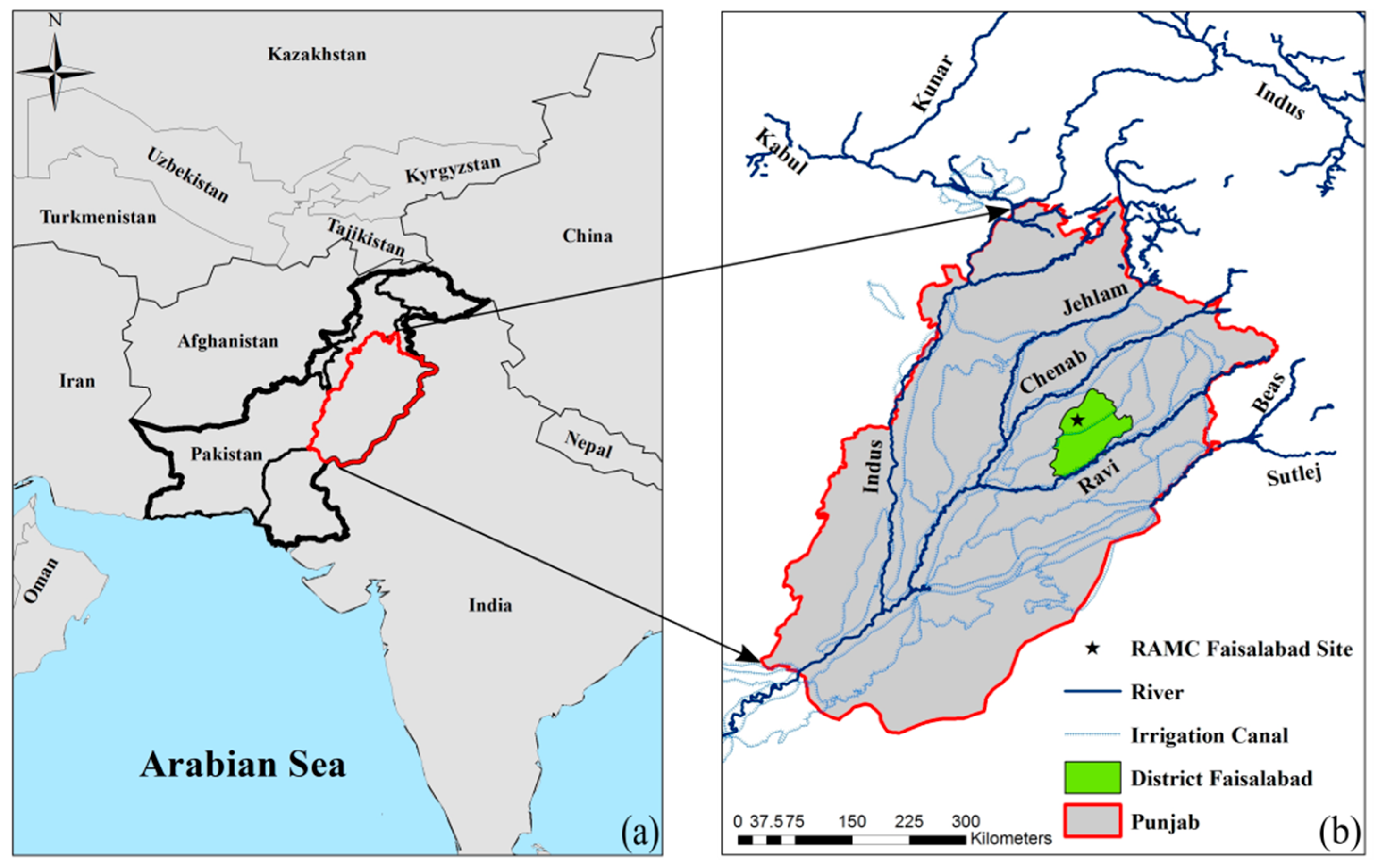
Figure 1. Location of (a) Punjab and (b) study site in district Faisalabad.
Agronomy 09 00744 g001
Figure 2. Methodological framework followed in this study for estimating the future wheat yield variability and water footprints.
Agronomy 09 00744 g002
Figure 3. Trends of wheat seasonal average (a) minimum temperature (Tmin), (c) maximum temperature (Tmax); and seasonal cumulative (e) solar radiation (Rn) and (g) rainfall (P) during 1980–2017 (left-hand panel). The right-hand panel (Figure 3b,d,f,h) shows the deviations of Tmin, Tmax, Rn and P from their respective long-term (1980–2017) averaged values during each wheat season. Red lines in Figure 3ah show the trends of the climate variables and the grey region represents the 95% confidence interval.
Agronomy 09 00744 g003
Figure 4. Trends of (a) wheat production, (c) cultivation area and (e) yield during 1980–2017. The right-hand panel (Figure 4b,d,f) shows the deviations of the three variables from their respective long-term (1980–2017) averaged values during each wheat season. Red lines in Figure 4ac show the trends of the climate variables and the grey region represents the 95% confidence interval.
Agronomy 09 00744 g004
Figure 5. (a) Wheat yield sensitivity to maximum temperature (Tmax), minimum temperature (Tmin), solar radiation (Rn) and rainfall (P); and (b) relative contribution of Tmin, Tmax, Rn and P to wheat TY_cli during the 1980–2017. The sensitivity values of Rn and P are multiplied by 100 for better visualization.
Agronomy 09 00744 g005
Figure 6. Monthly-, seasonal- and annual-scale variability of (a) maximum temperature (Tmax), (c) minimum temperature (Tmin), (e) solar radiation (Rn) and (g) rainfall (P) during the baseline (1980–2010), the 2030s (2021–2050) and the 2060s (2051–2080). The right-hand panel (Figure 6b,d,f,h) shows the change of average baseline Tmax, Tmin, Rn and P during the future time slices. The boxes in Figure 12a–h represent the inter-quartile range (IQR), the whiskers extend up to 1.5 times the IQR, the dots and horizontal lines inside the boxes represent mean and median, respectively, and outliers are shown as hollow dots outside the boxes. Monthly values are plotted on the left y-axes and seasonal and annual values are plotted on the right y-axes.
Agronomy 09 00744 g006
Figure 7. Average growing season length (GSL), reference crop evapotranspiration (ETo), actual crop evapotranspiration (ET), rainfall (P) and net irrigation water requirement (NIWR) for wheat during the baseline and future time slices. Each bar compares the baseline average values with the mean value of nine GCMs.
Agronomy 09 00744 g007
Figure 8. Projected changes in wheat-seasonal cumulative (a) reference crop evapotranspiration (ETo), (b) actual crop evapotranspiration (ET) and (c) net irrigation water requirements (NIWR) during the future time slices. The boxes in Figure 8a–c represent the inter-quartile range (IQR), the whiskers extend up to 1.5 times the IQR, the dots and horizontal lines inside the boxes represent mean and median, respectively, and outliers are shown as hollow dots outside the boxes. Each box shows the difference of baseline average values with the mean value of nine GCMs.
Agronomy 09 00744 g008
Figure 9. Projected wheat yield under future climate change during the two time slices.
Agronomy 09 00744 g009
Figure 10. Composition of wheat total water footprints (WFtotal) in terms of grey (WFgrey), blue (WFblue), and green water footprints (WFgreen) from 2004–2017.
Agronomy 09 00744 g010
Figure 11. Composition of wheat total water footprints (WFtotal) in terms of grey (WFgrey), blue (WFblue), and green water footprints (WFgreen) during the baseline and future time slices.
Agronomy 09 00744 g011
Figure 12. Projected changes in (a) green water footprint (WFgreen), (b) blue water footprint (WFblue), (c) grey water footprint (WFgrey) and (d) total water footprints (WFtotal) for wheat during the future time slices. The boxes in Figure 12ad represent the inter-quartile range (IQR), the whiskers extend up to 1.5 times the IQR, the dots and horizontal lines inside the boxes represent mean and median, respectively, and outliers are shown as hollow dots outside the boxes. Each box shows the difference of baseline average values with the mean value of nine GCMs.
Agronomy 09 00744 g012
Table 1. Summary of global circulation models (GCMs) used in the study.
GCMInstitutionHorizontal Resolution
BCC-CSM-1.1Beijing Climate Center, China Meteorological Administration~1.25° × 1.875°
BNU-ESMCollege of Global Change and Earth System Science, Beijing National University~2.8° × 2.8°
GFDL-ESM2MNOAA/Geophysical Fluid Dynamic Laboratory (GFDL)~2.0° × 2.5°
CCSM4US National Center for Atmospheric Research~0.9° × 1.25°
HadGEM2-ESUK—Meteorological Office—Hadley Center~1.25° × 1.875°
inmcm4Russian Institute of Numerical Mathematics (INM)~1.5° × 2.0°
MIROC5University of Tokyo, Japanese National Institute for Environmental Studies (NIES), and Japan Agency for Marine-Earth Science and Technology (JAMSTEC)~1.4° × 1.4°
MPI-ESM-LRMax Plank Institute of Technology (low resolution)~1.9° × 1.875°
MPI-ESM-MRMax Plank Institute of Technology (mixed resolution)~1.9° × 1.875°