Article

Deficit Irrigation as a Sustainable Practice in Improving Irrigation Water Use Efficiency in Cauliflower under Mediterranean Conditions

by
Abdelsattar Abdelkhalik
1,2,
Bernardo Pascual
1,3,*,
Inmaculada Nájera
4,
Carlos Baixauli
4 and
Nuria Pascual-Seva
1,3
1
Plant Production Department, Universitat Politècnica de València, Camí de Vera s/n, 46022 Valencia, Spain
2
Horticulture Department, Faculty of Agriculture, Fayoum University, 63514 Fayoum, Egypt
3
Valencian Centre for Irrigation Studies, Universitat Politècnica de València, Camí de Vera s/n, 46022 Valencia, Spain
4
Cajamar Experimental Centre in Paiporta, Camino del Cementerio Nuevo s/n, 46200 Valencia, Spain
*
Author to whom correspondence should be addressed.
Agronomy 2019, 9(11), 732; https://doi.org/10.3390/agronomy9110732
Submission received: 6 September 2019 / Revised: 24 October 2019 / Accepted: 7 November 2019 / Published: 8 November 2019
(This article belongs to the Special Issue Increasing Agricultural Water Productivity in a Changing Environment)

Abstract

:
Water shortage is one of the major constraints in vegetable production. Deficit irrigation is a sustainable technique that improves irrigation water use efficiency. Field studies were conducted during two growing seasons to evaluate the effects of deficit irrigation on plant growth, plant water status, productive response (curd yield and quality), irrigation water use efficiency (IWUE), and crop profitability of cauliflower. Nine irrigation treatments were used, applying 100%, 75% (moderate), or 50% (severe) of the irrigation water requirements (IWR) during the entire growing season (Continued Deficit Irrigation, CDI), or 75% and 50% of IWR during one of the following stages (Regulated Deficit Irrigation, RDI): Juvenility, curd induction, and curd growth. Severe deficit irrigation applied during juvenility and curd induction reduced the plant size, but it only led to a significant reduction of marketable yield (22%), and average curd size and weight if it was maintained throughout the crop cycle, supposing the highest IWUE (43.6 kg m−3). Moderate CDI or severe RDI during juvenility did not reduce significantly the curd yield compared to fully irrigated plants (4.4 kg m−2), thereby obtaining similar gross revenues (16,859 € ha−1) with important water savings (up to 24.3%), improving IWUE (up to 34.2 kg m−3).

1. Introduction

Cauliflower (Brassica oleracea var. botrytis L.) is an important vegetable crop worldwide, particularly in the Mediterranean area [1]. It has an important role in the human diet, with medicinal and functional properties [2]. Cauliflower has a great economic importance; the global cultivated area of cauliflower and broccoli in 2017 was about 1.40 × 10⁶ ha. and produced approximately 2.6 × 10⁹ kg of curds. Globally, China is the largest producer of cauliflower, followed by India and the USA [3]. Spain is ranked fourth in the world, and first in Europe for cauliflower and broccoli production, and during the last decade it has been the world’s first exporter [3].
Sustainable water management is a key objective of sustainable agricultural practices, given that agriculture accounts for the major share of total water use, approximately 69% of the global freshwater withdrawals [4]. Drought stress is one of the major constraints threatening crop production [5]. Water shortage is becoming critical in arid and semi-arid areas of the world, including the Mediterranean area [6,7]. The demand for water is expected to increase in the future, particularly with the foreseen growth of the world population, the increase of irrigated agriculture areas, and climate change [8,9,10].
Deficit irrigation (DI) is considered to be a sustainable practice, and has been developted to improve water productivity, minimize yield losses, and even improve product quality [11,12]. Deficit irrigation consists of applying irrigation below the optimum crop water requirements, either, during the whole growing season (continued DI; CDI) or at specific phenological stages, when the crop is less sensitive to water stress (regulated DI; RDI) [6,11,13,14].
The plant response to DI depends upon timing, duration, and the magnitude of water restriction [5,6,14], and it is crop-specific. Therefore, DI requires precise knowledge of the crop yield and quality response to water stress [15]. At present, the aim of researchers and growers is, not only to increase crop yield, but also to maximize irrigation water use efficiency [16].
Cauliflower is generally considered to be a sensitive crop to water stress, and such susceptibility has been documented in several reports, such as by Kochler et al. [17] in Germany, Sarkar et al. [18,19] in India, and Pereira et al. [20] in Brazil. Bozkurt et al. [21], and Souza et al. [22] studied different irrigation levels below, and above, optimum irrigation.They obtained the highest yield with full irrigation, while excess water applications had a negative effect on the yield of cauliflower. According to Latif et al. [23], water stress reduced plant growth, leaf chlorophyll concentration, relative water content, and protein content of cauliflower cultivated under net-house conditions in Iran.
In contrast, Seciu et al. [24] pointed to cauliflower having an intermediate susceptibility to water deficits. Cauliflower yield losses, observed by Thompson et al. [25] during three field experiments in southern Arizona were, to a great extent, the consequence of excessive irrigation rather than of deficit irrigation. Obviously, plant responses to water deficits vary with the season, region, cultivar, and stress patterns. Currently, there is little available data on cauliflower response to different levels and timing of water deficits under Mediterranean conditions, especially for developed hybrids. Therefore, it is important to evaluate the sensitivity of cauliflower to water deficits at various stages, in order to determine the optimal timing to apply water reductions.
The main aim of this research is to evaluate the effects of continued and regulated deficit irrigation on plant growth, plant water status, productive response (in terms of yield and curd quality), irrigation water use efficiency (IWUE), and crop profitability of cauliflower grown under Mediterranean conditions.

2. Materials and Methods

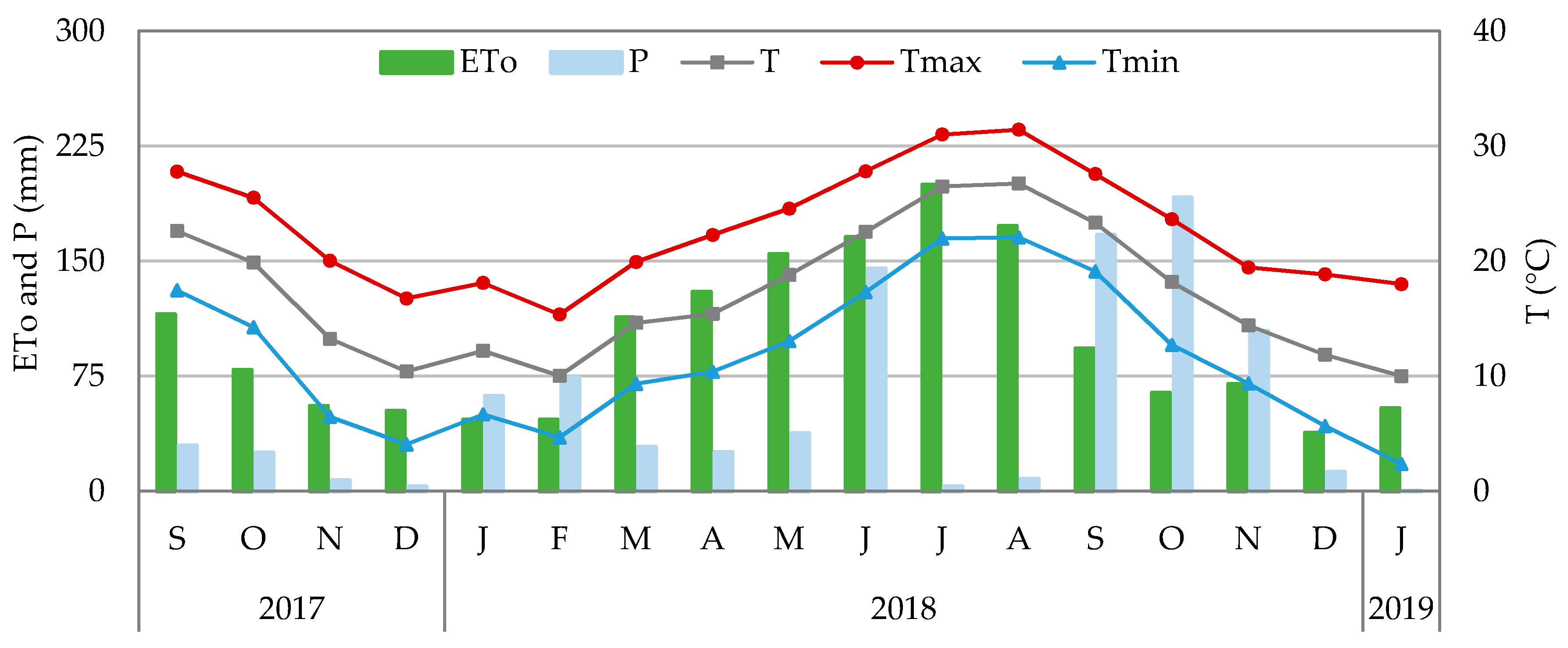
2.1. Experimental Site Conditions

Two experiments were conducted during two successive growing seasons (2017 and 2018) at the Cajamar Experimental Centre in Paiporta, Valencia, Spain (39.4175 N, 0.4184 W, 52 mamsl). To avoid soil replanting disorders, resulting from serial cauliflower cropping, two subplots within the experimental plot were used. It was part of a crop rotation that consisted of sweet pepper, onion, watermelon and cauliflower, in the indicated order for both years. The soils were deep, with a medium (silt loam) texture, which were classified as Petrocalcic Calcixerepts according to the USDA Soil Taxonomy [26]. The soil analyses indicated that the soil of the two subplots were similar, being very slightly alkaline (pH = 7.6–7.7), and highly fertile [organic matter = 2.0–2.1% with high available phosphorous (42–43 mg kg−1; Olsen) and potassium (445–503 mg kg−1; ammonium acetate extract) concentrations]. Irrigation water was pumped from a well, with (on average) EC 1.96 dS m−1 and 77 mg kg−1 N-NO3− content.
Figure 1 shows climatological data of the growing seasons. Temperatures registered in October 2017 and January 2018 were higher than those registered in October 2018 and January 2019, respectively (particularly average and minimum temperatures; Figure 1). However lower temperatures were registered in November and December in 2017 than in 2018. Reference evapotranspiration (ETo) was determined according to Allen et al. [27], as follows,
ET O   =   E pan ×   K p
where Epan (mm day−1) is the evaporation from a class A pan installed adjacent the Experimental Center and Kp (0.815) is the pan coefficient determined according to Allen et al. [27]. Greater ETo values were obtained in 2017 than in 2018, in the first part of the growing season (September and October; Figure 1), while higher water demands were estimated in January 2018 than in January 2019 (Figure 1). According to Papadakis’s agro-climatic classification [28], the climate is subtropical Mediterranean (Su, Me), with hot and dry summers and an average annual rainfall of approximately 450 mm, irregularly distributed throughout the year. It is worth highlighting the precipitations registered in June, September, October, and November 2018, with monthly values greater than 100 mm.

2.2. Crop Management and Plant Material

The cauliflower ‘Naruto F1’ (Clause®) was used in the experiments, due to its adaptation to the soil and climate conditions in the area, and to its high productivity, as evaluated at Cajamar Experimental Centre [29]. The curds are round, uniform, dense, and bright white, with an excellent behavior for both the fresh market and for the industry. Plants are vigorous, with a strong foliage that protects the curd.
The seeds were sowed on 8 August 2017 and 11 August 2018, in polystyrene trays of 126 cells, in a peat moss-based substrate (70% blonde and 30% dark), that has been recommended for vegetable seedbeds (Pindstrup Mosebrug S.A.E., Sotopalacios, Spain). They were maintained in a Venlo-type greenhouse. Seedlings were transplanted on 12 September 2017 and 24 September 2018, when they reached the four-leaf stage, in an open-field in flat raised beds, which were separated 1 m apart between the bed centers, being the raised bed 0.6 m wide and 7.25 m long. Plants were placed following a staggered pattern, 0.66 m apart (30,300 plants ha−1). Each experimental plot consisted on 3 flat raised beds, being the central one (22 plants) used for yield and plant determinations, and the lateral ones to avoid interferences. The incorporation of nutrients (200-80-200 kg ha−1 N-P2O5-K2O) was performed by fertigation, following the criteria indicated by Pomares et al. [30].

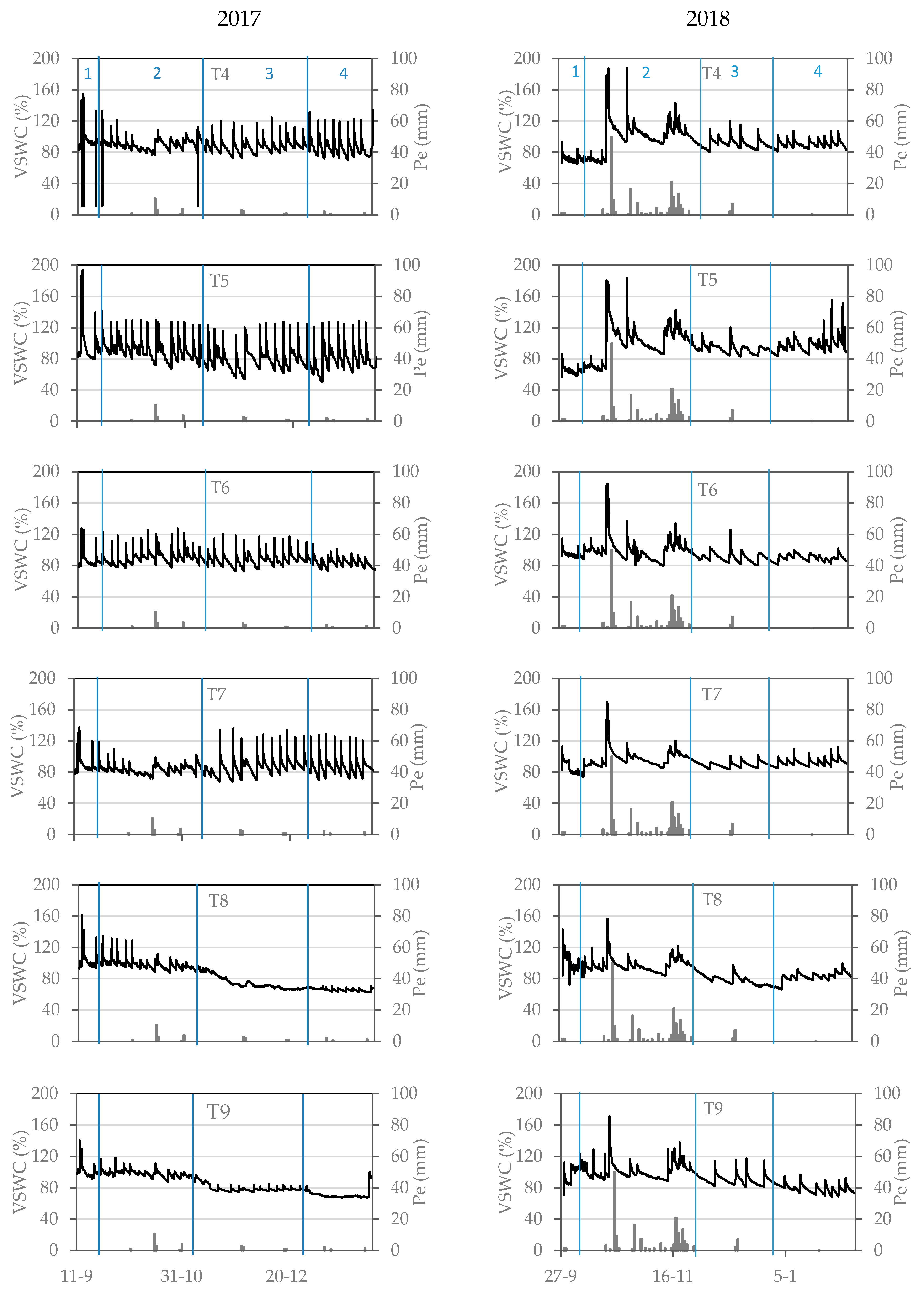
2.3. Deficit Irrigation Strategies and Growth Stages

The cauliflower growth period was divided into four stages [1,31]: (1) Initial, from transplanting to plant establishment; (2) juvenility, from establishment until the plant forms a critical number of leaves (12–15 leaves for the used cultivar); (3) curd induction, until the appearance of the curd (until approximately 4 cm diameter; cauliflower responds to relatively low temperatures from this physiological age, inducing curd formation); and (4) curd growth, extending from the end of phase 3 until the end of the harvest. These four growth stages coincide with those defined for crop coefficient (Kc) by Allen et al. [27]: (1) Initial, (2) crop development, (3) mid-season stage, and (4) late-season stage. Table 1 shows the duration and the irrigation water applied (IWA) for each growth stage. Initially, all the treatments were irrigated with 30 and 26 mm in 2017, and 2018, respectively, to ensure adequate plant establishment. Then, different irrigation strategies were initiated.
The experiments consisted of nine irrigation strategies (IS) in the two growing seasons (GS). The analyzed IS, included T1, T2, and T3 applying 100%, 75%, and 50% of the irrigation water requirements (IWR), respectively, throughout the GS; T4, T5, and T6 reduced IWA to 75% of the IWR during the crop growth stages, 2, 3, and 4, respectively; T7, T8, and T9 reduced the water applied to 50% of the IWR, at the same growth stages.

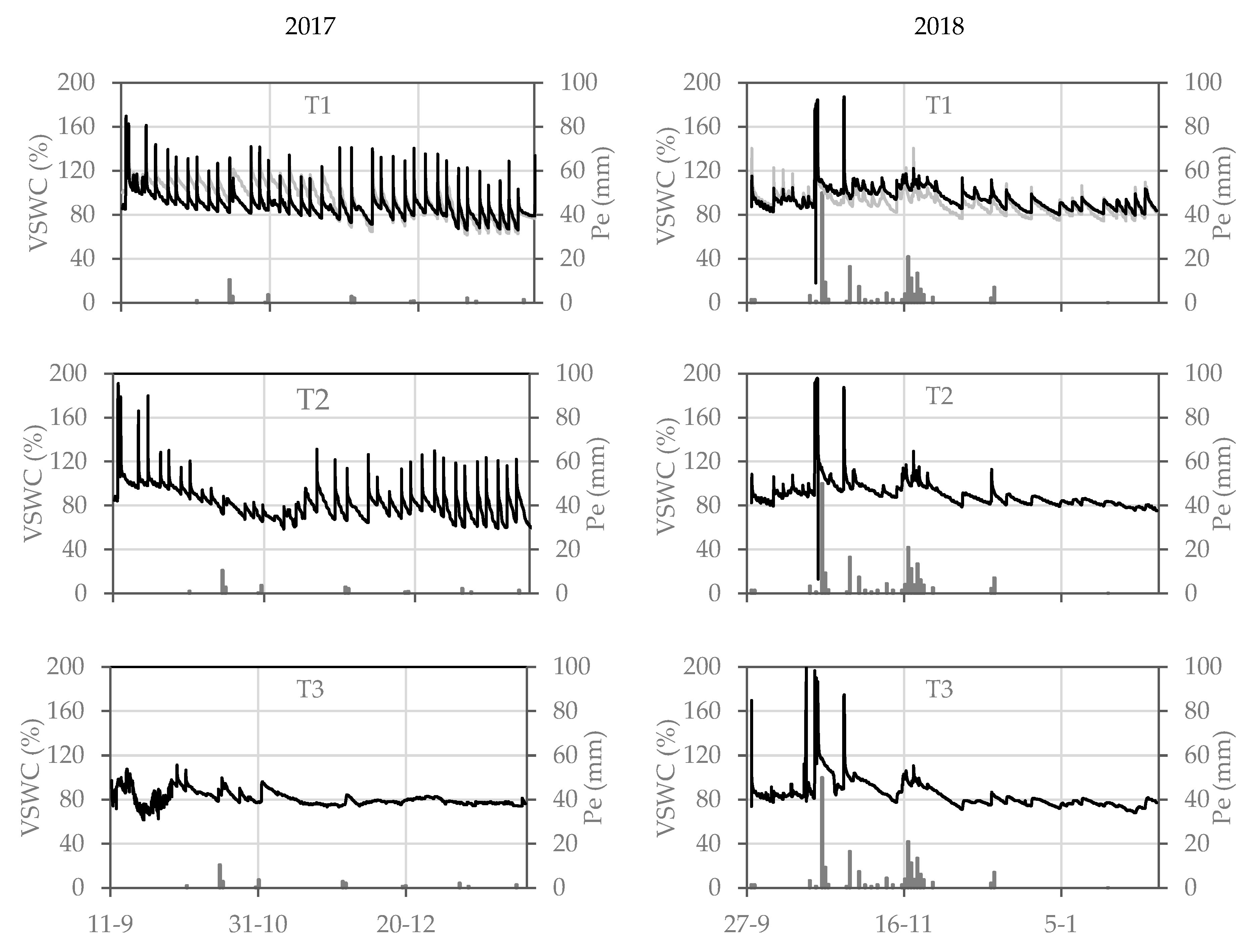
2.4. Volumetric Soil Water Content

The volumetric soil water content (VSWC; m3 m−3) was continuously monitored using ECH2O EC-5 capacitance sensors connected to an Em50 data logger, and using the ECH2O Utility software (Decagon Devices Inc., Pullman, WA., USA). Following the recommendations described by Sarkar et al. [19] and Pereira et al. [20], in each treatment, one sensor was installed horizontally at a depth of 0.15 m, in the middle of the beds below the dripline and equidistant between two adjacent emitters. Additionally, in T1, another sensor was placed at 0.30 m depth to verify that water losses at depth were unimportant. The VSWC was measured and stored at 15 min intervals, and the variations in the VSWC were used to determine the in-situ field capacity (FC). In order to compare the VSWC corresponding to the different IS and GS, their values have been presented as the ratio of the VSWC compared with the VSWC at FC (% FC).

2.5. Irrigation Scheduling and System

The IWR between two consecutive irrigation events was determined using the following equation,
IWR   = ET C Pe Ef
where ETc (mm) is the crop evapotranspiration, Pe is the effective precipitation (mm) determined from rainfall data using the method of the U.S. Bureau of Reclamation [32], as presented by Pascual-Seva et al. [33], and Ef is the irrigation efficiency of 0.95 (considering distribution uniformity = 0.99 and deep percolation ratio = 0.04 which is comparable to leaching requirement, as it has been stated for cauliflower cultivars grown in the Experimental Centre [30]).
The ETc (mm) was calculated from the ETo and a single Kc proposed for local conditions by the IVIA [34], adapting the duration of each stage to the growing cycle:
ET C =   ET O   ×   K c .
Kc values were 0.7, 1.0, and 0.9, corresponding to initial, mid-season, and late season stages. The irrigation water was supplied by a drip irrigation system with one lateral line per bed, using a turbulent flow dripline (16 mm; AZUDRIP Compact; Sistema Azud S.A., Murcia, Spain) with emitters spaced 0.33 apart and a discharge rate of 2.2 L h−1. An irrigation controller programmer (NODE-100 single station controller, Hunter, CA, USA) was connected to the irrigation system for programming the irrigation events. A water flow meter (MJ-SDC TYP E, NWM, Czech Republic) was connected to each IS, to record the IWA. The irrigation events for the all the IS began when the VSWC in T1 descended to 80% of FC (thereby avoiding the effect of the irrigation frequency between IS), applying in each strategy its corresponding IWA. This irrigation management was proved to be adequate in a preliminary study carried out in the same Experimental Centre with the same cultivar (unpublished data).

2.6. Relative Water Content and the Membrane Stress Index

The relative water content (RWC; %) and the membrane stress index (MSI; %) were evaluated at the end of each stage. Leaf RWC was determined in fresh leaf discs of 2 cm diameter using the method developed by Barrs [35], and it was calculated using the following equation (Hayat et al. [36]),
RWC   ( % ) =   ( FW DW ) ( TW DW )   ×   100
where FW, DW, and TW are the disc fresh weight, dry weight, and turgor weight, respectively.
The MSI was determined using 0.2 g samples of fully expanded leaf tissue, following the methodology described by Rady [37], and it was calculated as,
MSI   ( % )   = ( 1 C 1 C 2 )   ×   100
where C1 is the electrical conductivity of the solution after the samples were heated at 40 °C in a water bath for 30 min, and C2 is the electrical conductivity of the solution after the samples were boiled at 100 °C for 10 min.

2.7. Plant Growth and the Harvest Index (HI)

Growth parameters were evaluated at the end of plant growth. Plant height and diameter, leaf number per plant, and chlorophyll index (SPAD) were determined in the field, with four plants each plot. The SPAD was measured at three points, in three fully developed leaves in each plant, using a SPAD-502 m (Konica Minolta Sensing Inc., Tokyo, Japan), considering the average values for each plant. The aboveground parts of the plants were divided into two parts and analyzed separately: Vegetative, including stem and leaves (hereinafter referred to as shoots), and reproductive, the curd. Each sampled plant part (shoots and curd) was weighed with an analytical balance (Mettler Toledo AG204; Greifensee, Switzerland); thereafter, they were dried at 65 °C in a forced-air oven (Selecta 297, Barcelona, Spain) until they reached a constant weight, to obtain the dry weights. The harvest index (HI) was determined as the ratio of curd to total aboveground biomass on a dry mass basis (g g−1; [38]).

2.8. Curd Yields, Irrigation Water Use Efficiency (IWUE), and Yield Response Factor (Ky)

In 2017, the harvest was completed in five passes between 12 and 29 January 2018, and in 2018, it started on 17 January 2019 and lasted until 04 February 2019, requiring six passes. The yield components were determined from a 5 m length (15 plants) of the central part of the bed, leaving the plants on each side to avoid marginal effects. Total curd yield was partitioned into marketable (MY) and non-marketable yield. The MY was considered “with leaves” [39]. The non-marketable yield included curds that were small (lower than 700 g) or that presented defects in shape (lack of compactness, or premature opening), that were the only culls found.
The IWUE was calculated as the ratio of MY (fresh mass; kg m−2) to IWA (m3 m−2; [40]). The yield response to water deficits during the crop cycle was determined according to Doorenbos and Kassam [41], using the following equation,
( 1 Y a Y m )   =   K y ( 1 ET a ET m )
where Ya and Ym are the actual MY (corresponding to the different DI strategies), and maximum MY (fully irrigated plants), respectively; ETa and ETm are the actual (DI), and maximum (full irrigated) ET (mm), respectively; and Ky is the yield response factor, which was obtained by lineal regression for each stage. For each IS, ET was obtained from the corresponding IWA and Equation (2).

2.9. Physical Properties and Color Indices of the Curds

Curd physical attributes and color indices were assessed during the second harvest in both GS. Three representative curds per plot were selected to determine perimeter with a flexible measuring tape. Then, curd color was measured using a chroma meter (Minolta CR-300; Konica Minolta Sensing Inc., Tokyo, Japan) and the CIELAB (CIE 1976 L*a*b*) color space coordinates were obtained from three readings performed at the curd surface (in the center and the two ends of the maximum diameter). The average values were used to calculate the following color indices. L represented curd brightness. Hue angle (H°) was calculated as described by McGuire [42]:
H °   =   arctang   ( b a ) + 180 .
Chroma (C*) was calculated as stated by Pathare et al. [43]:
C   =   ( a 2 + b 2 ) .
Curd firmness was determined using a digital penetrometer with a tip of 8 mm diameter (Penefel DFT 14, Agro Technologies, Forges les Eaux, France). Later, these curds were cut to determine curd size (height and diameter) using a measuring tape.

2.10. Profitability

The gross revenue (money generated by the sale of the cauliflower curds) and economic value of water (money generated by m3 of IWA) were calculated by multiplying the average values of MY, and IWUE, respectively, by the average cauliflower curd price corresponding to the last three years (0.38 € kg−1) [44].

2.11. Experimental Layout and Statistical Analysis

The experiment was performed in a randomized complete block design in three replicates. The results were evaluated by analysis of variance (ANOVA) using Statgraphics Centurion XVII [45]. The percentage data were arcsin transformed before analysis. Least significant differences (LSD) at a 0.05-probability level were used as the mean separation test. MY and IWUE were related with IWA using Statgraphics Centurion XVII [45].

3. Results

3.1. Growth Stages and Irrigation Water Applied

The total growth cycle period (including the initial period) was 140 days in 2017 and 134 days in 2018. The total pan evaporation and ETo were higher in 2017 (326, and 266 mm, respectively) than in 2018 (226, and 184 mm, respectively). The total and effective precipitation varied between GS, being much higher in 2018 (475, and 177 mm, respectively) than in 2017 (126, and 30 mm, respectively). The IWA values during the differential irrigation periods ranged from 113 (T3) to 224 mm (T1) in 2017, and from 57 (T3) to 113 mm (T1) in 2018 (Table 1).

3.2. Volumetric Soil Water Content

Figure 2 and Figure 3 show the VSWC (expressed as % FC) for the different IS at 0.15 m (and 0.30 m for T1) depths, as well as the daily rainfall during the growing seasons. The VSWC at 0.15 m depth varied between the GS, with higher values in 2018 (on average 91.5% FC) than in 2017 (on average 84.9% FC). Furthermore, it can be observed that VSWC in 2017 registered larger oscillations for each irrigation event than in 2018. This different behavior may be related to the sensitivity of the capacitance sensors to the soil conditions in the area immediately surrounding the sensor (i.e., air gaps, compaction or variation in the soil) [46]. The slight increments of the VSWC values at 30 cm depth (in T1) are related to slight deep percolation, which are consistent 4% deep percolation considered in the irrigation management. The average VSWC at 0.15 m depth in 2017 ranged between 88.2% (T1) and 81.0% FC (T3), and in 2018 between 95.2% (T1) and 84.8% FC (T3). In both GS, except when important rainfall occurred, i.e., stage 2 in 2018, a slight reduction in VSWC at 0.15 m was registered in the phases when the restriction was applied, particularly with severe water deficits (50% IWR).

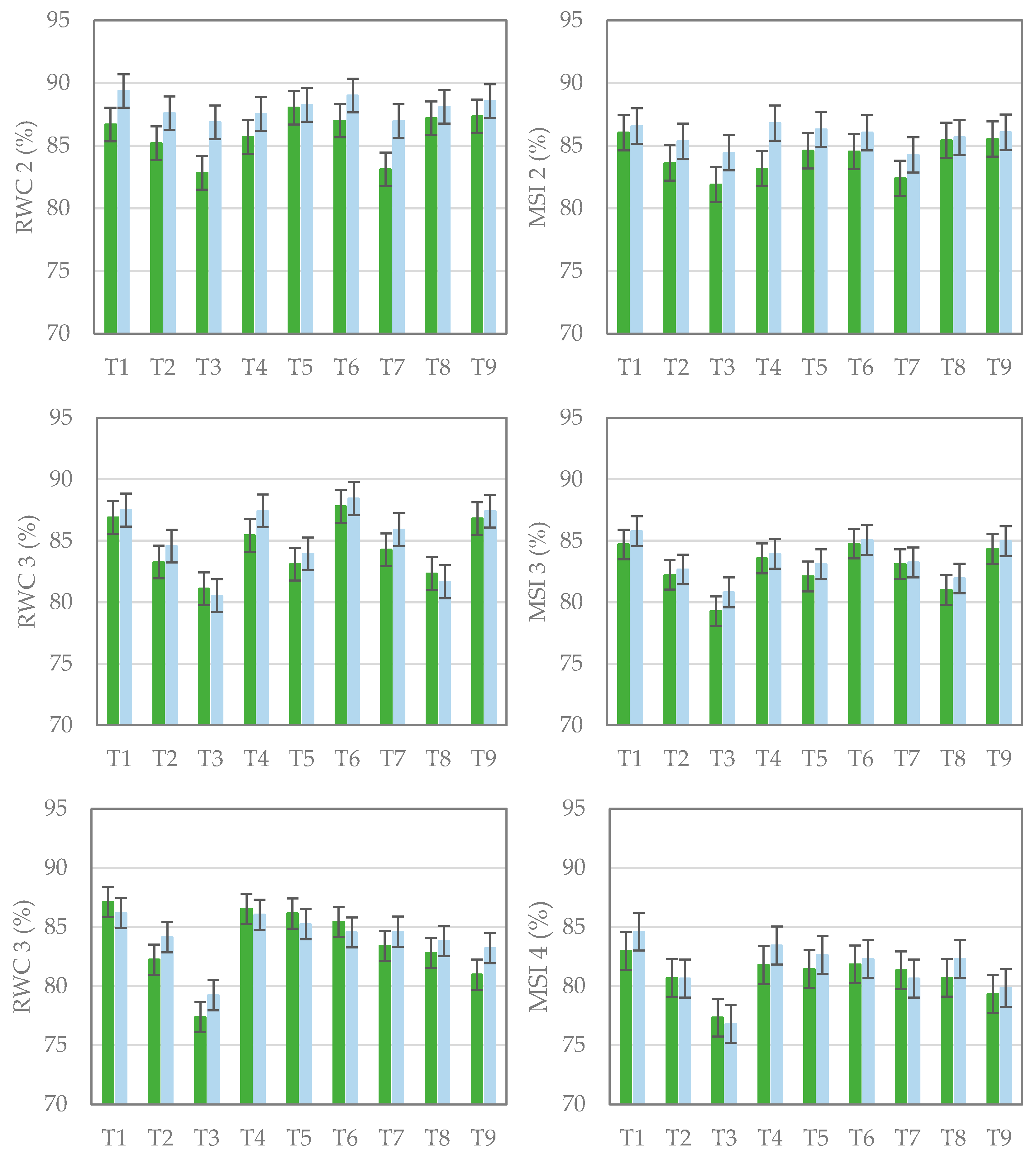
3.3. Relative Water Content (RWC) and the Membrane Stability Index

The effects of GS and the IS on cauliflower RWC and MSI indices are presented in Figure 4. At the end of juvenility, both parameters were affected by both the GS (p ≤ 0.01) and the IS (p ≤ 0.01/0.05), in the sense that higher values were found during 2018 (87.9, and 85.7, respectively) than during 2017 (85.9, and 85.7, respectively), but this difference was not observed in the following stages. At the end of juvenility, the lower values (p ≤ 0.05) were obtained with the IS that had been exposed to water restrictions in that stage (particularly in 2017 with the most severe strategies; T3 (82.8) and T7 (83.1)). At the end of the curd induction and curd growth stages, both RWC and MSI were negatively affected (p ≤ 0.01) by the IS. The lowest values were obtained with the most restrictive CDI (T3), followed by the plants that were exposed to severe water restrictions at the corresponding stage (T8 in stage 3 and T9 in stage 4).

3.4. Plant Growth and Harvest Index (HI)

Cauliflower growth was significantly affected (p ≤ 0.05) by the GS and the IS (Table 2), but not by their interaction. The plants that were grown in 2017 were higher and wider (p ≤ 0.01) than those grown in 2018, but they presented a similar number of leaves. Regarding the IS, the shortest plants were obtained with the most restrictive CDI (T3), followed by the moderate CDI (T2), not differing from plants exposed to water restriction during the juvenility and curd induction stages (T4, T5, T7 and T8). Plants with lower width were also obtained with T3, not differing from T7 and T8. The lowest number of leaves per plant was found in CDI (T3 and T2).
Higher values of SPAD (p ≤ 0.01; Table 3) were reported in 2017 (64.6) than in 2018 (60.8), not being affected by the IS. Heavier plants were obtained in 2017 than in 2018 (p ≤ 0.01). IS did not affect the shoot weight) but it did reduce the curd dry weight (p ≤ 0.05). The curd dry weight decreased significantly (p ≤ 0.05) with CDI (0.323, 0.294 and 0.265 for T1, T2, and T3 respectively) and severe water stress at curd induction (T8; 0.272). The GS affected (p ≤ 0.01) the HI, with the highest value obtained in 2018, while the IS did not affect it (p > 0.05).

3.5. Curd Yields, Irrigation Water Use Efficiency (IWUE), and Yield Response Factor (Ky)

Cauliflower curd yield was affected (p ≤ 0.01; Table 3) by the GS, representing 73.1%, 63.1% and 71.9% of the sum of squares of total yield, MY and average curd weight, respectively, with higher values in 2017. Yield was not affected (p > 0.05) by IS; regarding MY, T3 led to the lowest value (p ≤ 0.05), whereas the other strategies did not differ from full irrigation (T1), as observed for the average curd weight (p > 0.05). The non-marketable yield was not affected (p > 0.05; data not shown) by the GS or by the IS. IWUE was significantly influenced (p ≤ 0.01) by both GS and IS, with the greatest IWUE in 2018 and severe CDI (T3), followed by moderate CDI (T2) and reducing IWA to 50% during juvenility (T7).
Considering the average MY and IWA values at the total cycle (CDI), or at each stage separately in both GS, MY increased linearly with increasing IWA either during the whole GS (CDI) or at each stage when the water restriction was applied, as presented in the following equations:
  • CDI: MY = 2.4080 + 0.0126 IWA (r = 0.90; p ≤ 0.01)
  • Juvenility: MY = 2.5289 + 0.0119 IWA (r = 0.88; p ≤ 0.01)
  • Curd induction: MY = 2.4596 + 0.0115 IWA (r = 0.84; p ≤ 0.01)
  • Curd growth: MY = 2.4463 + 0.0116 IWA (r = 0.69; p ≤ 0.01).
The IWUE decreased linearly with increasing IWA, according the following equations:
  • CDI: IWUE = 55.7151 − 0.1606 IWA (r = −0.91; p ≤ 0.01)
  • Juvenility: IWUE = 49.5329 − 0.1234 IWA (r = −0.88; p ≤ 0.01)
  • Curd induction: IWUE = 46.2573 − 0.1092 IWA (r = −0.89; p ≤ 0.01)
  • Curd growth: IWUE = 46.6245 − 0.1109 IWA (r = −0.91; p ≤ 0.01).
Regarding Ky, considering the CDI for the two GS, its value was 0.56.

3.6. Physical and Color Indices of the Curds

The physical properties and color indices of cauliflower curds in response to the IS and GS are shown in Table 4. Curd size (height, diameter and perimeter) was significantly affected (p ≤ 0.01) by the two analyzed factors, GS and IS. Higher values were obtained in 2017, and regarding the IS, plants cultivated under the severe CDI strategy (T3) recorded the lowest values, while those subjected to full irrigation (T1) recorded the highest values, without significant differences with the other IS. Curd dry matter content and curd firmness were affected (p ≤ 0.05) by GS, with 2017 showing the highest values of dry matter content and the lowest of firmness. Color indices (H°, C* and brightness) were influenced (p ≤ 0.01/0.05) by the GS, with higher H° and C* and lower L values in 2018, but none of these parameters were affected (p > 0.05) by the IS.

3.7. Profitability

The gross revenue and water economic value were affected by the GS and IS (Table 5). The highest gross revenue and lowest water economic value were obtained in 2017 (p ≤ 0.01). Severe CDI (T3) led to the lowest gross revenue (p ≤ 0.05; 13,161 € ha−1) and the highest water economic value (p ≤ 0.01; 16.56 € m−3).

4. Discussion

Juvenility is usually the longest stage in cauliflower autumn and winter production, occurring during September and October, when temperature and evapotranspiration are higher, compared to the later stages, the IWR (IWA for T1; Table 1) were higher at this stage. The lower IWA in 2018 was due to both the lower evaporative demands and the higher incidence of precipitation (Figure 1). The differences between IWA in different years were also reported by Bozkurt et al. [20] in Turkey, and Kałużewicz et al. [47] in Poland. IWA in full irrigation strategy (T1) in 2017 is similar to that reported in [20] (212 mm for 2006), while the IWA in 2018 is similar to that reported in [47] (104 mm for 2012 and 2013).
The VSWC recorded at 0.15 m depth in 2018 (on average 91.5% FC) were higher than that in 2017 (on average 84.9% FC). This difference may be mainly related to the higher precipitation registered in 2018, particularly that which occurred in October and November. The full irrigation strategy (T1) recorded the greatest average VSWC over the two years. In both GS, a decrease in VSWC values was observed during the corresponding restriction phase, particularly for severe water reductions, recovering when full irrigation was restored. Costa et al. [11] and Du et al. [16] reported that an early plant response to soil water drying is stomatal closure (which may start during moderate water shortages), and is regulated (among other factors) by hormonal signals (ABA), which are transported from dehydrated roots to the leaves, impacting directly on plant water status and carbon exchange.
The MY obtained in the present study (5.02 kg m−2 in 2017 and 3.85 kg m−2 in 2018) is similar to those obtained (3.48 kg m−2 in 2017 and 4.08 kg m−2 in 2018) in other experiments conducted with standard conditions [27] (full irrigation) in the Experimental Centre [29].
Leaf water status depends upon the VSWC, which can become a stressor [48]. At the end of juvenility both RWC and MSI were higher (p ≤ 0.05) in 2018 than 2017, but this difference was not significant (p > 0.05) in the later stages, due to the small VSWC differences between GS, as previously indicated. Regarding IS, fully irrigated plants showed the highest RWC and MSI during the whole growing period (T1), while the lowest values in each phase were obtained for the strategies that reduced the water applied in the corresponding phase, particularly at severe levels (50% of the IWR). The RWC and MSI obtained in this study were in agreement with those reported by Wu et al. [49] and Latif et al. [23]. The differences in RWC and MSI, between the full irrigation strategy (T1) and the most restricted CDI (T3), could explain the reduction that the CDI causes in the growth and MY. As previously cited, an initial effect of decreased soil water availability is stomatal closure, which reduces carbon uptake by leaves, and limits photosynthetic activity, consequently leading to a reduction of plant growth [48,50]. Severe water stress leads to RWC and MSI reductions, inducing modifications in the relative rates of photosynthesis and respiration, and even leading to photosynthesis ceasing, respiration increasing, and abscisic acid accumulation [51].
Plant growth, expressed as plant size (height and diameter) and leaf number, was negatively affected (p ≤ 0.01) by water deficits, getting the lower values with CDI (T3 and T2) and severe water restriction at juvenility (T7) and curd induction (T8). Similarly, Souza et al. [22] recorded lower values of plant height and leaf number of cauliflower, grown under water stress at 40% ETc, compared to higher irrigation levels.
In this study, IS did not alter HI. Similar results were reported by Bozkurt et al. [21], who only observed lower HI values with non-irrigated cauliflower, compared to the application of 0.75 and 1.0 of evaporation from a Class A pan. According to Fereres and Soriano [12], moderate water deficits lead to reduced biomass production, while dry matter partitioning is usually not affected and the HI is maintained [12]. Although, more severe stress can affect the dry matter partitioning, thereby reducing HI.
Temperature has an important effect on growth and development of cauliflower plants. As Dixon [2] stated, initially the leaf initiation rate during juvenility is related to temperature; after juvenility, during curd induction, relatively low temperatures are required; but later, during curd growth, the diameter of the curd increases with temperature up to a maximum level. The greater plant size, shoot biomass and curd weight obtained in 2017 compared to 2018 could be related to the slightly higher temperatures registered during the juvenility and curd growth phases in 2017.
Severe CDI (T3) caused a significant reduction in the MY (22%) compared to full irrigation. While, it was not significant (p > 0.05), both T8 and T9 caused a 9% reduction in the MY compared to full irrigation. This reduction was related to the decrease of the average curd weight, and to a lesser extend to the increase of the non-marketable curds. Sarkar et al. [19] recorded the maximum cauliflower curd yield under irrigation at −0.03 MPa soil matric potential, and it decreased by 10.4% and 31.4% under −0.05 MPa, and −0.07 MPa, respectively. In this research MY decreased linearly with decreasing IWA for water restriction at the total growth cycle or at the different water restriction stages. Sarkar et al. [19] found a significantly linear relationship between curd yield and actual evapotranspiration with irrigation levels ranged between 0 and 125% Epan. Bozkurt et al. [21] found a significant second-degree polynomial relationship between the cauliflower yield and IWA, but they evaluated different irrigation levels from 0 to 1.25 of pan evaporation, exceeding the maximum crop water needs.
The greatest IWUE was obtained in 2018, mainly because the IWA in 2018 was approximately 50% that of 2017. Evidently, IWUE depends, among other factors, on the crop cycle and particularly on meteorological conditions. In relation to IS, the greatest IWUE was obtained with T3, which implies that the water savings (50%) were greater than the reduction of MY (22%) compared to full irrigation (T1). Furthermore, the CDI with 75% of the IWR (T2) and water deficits of 50% of the IWR during juvenility (T7) increased IWUE by 20.3%, and 20.7%, respectively, because of the important water savings in relation to T1, 24.3%, and 22.8%, respectively. According to Tolk and Howell [52], the greatest IWUE usually occurs at an ET that is generally less than the maximum ET, suggesting that irrigating to achieve the maximum yield would not correspond to the most efficient use of irrigation water, as found in this study. The IWUE values, obtained in the present research, are consistent with those obtained by Bozkurt et al. [21], who reported that IWUE increased with decreasing irrigation rate.
Ky values lower than 1 indicate that the crop is tolerant to water deficits [41,53]. The Ky obtained for CDI (0.56 on average for both GS) indicates that it is not very sensitive to water deficits. Similar Ky values were reported by Sarkar et al. [19], being 0.65, 0.86, and 0.77 for irrigation at −0.03 MPa, −0.05 MPa, and −0.07 MPa of the soil matric potential, respectively.
In this study, the curds produced by fully irrigated plants (T1) were the tallest and widest, and with the greatest perimeter, while severe CDI (T3) was the only strategy that reduced these dimensions (p ≤ 0.05). This is related to a decrease in average curd weight, and consequently a decrease of MY. These results agree with those obtained by Bozkurt et al. [21] and Souza et al. [22].
Cauliflower curd marketability improves with its whiteness. Curds produced in 2017 had higher values of L and lower values of H° and C* than those in 2018, indicating that they were whiter. In agreement with Wang et al. [54], the slight yellowish color of curds, produced in 2018, may be mainly related to the accumulation of chlorophylls and carotenoids, which in turn, may be related to the greater radiation registered during the curd growth stage (on average 9.7 MJ m−2 day−1 in 2018 and 7.0 MJ m−2 day−1 in 2017). These color indices were not affected by IS, and their values are consistent with those obtained by Gu et al. [55] and Wang et al. [54].
Adequate deficit irrigation management requires evaluation of the economic impact of the yield reduction, that has been produced by water stress [15]. This enables growers to decide on whether or not to implement water reduction. The potential profitability of the deficit irrigation could be achieved by increasing the IWUE or reducing irrigation costs [56]. Moderate CDI (T2) or severe water restriction at juvenility (T7) would lead to a slight decrease, not statistically significant (p > 0.05), in the gross revenue (8%, and 6%, respectively), even though increasing IWUE. Therefore the water economic value (20%, and 21%, respectively) is increased compared to full irrigation (T1). Reducing the water applied to 75% of IWR at juvenility (T4) caused a low reduction in the gross revenue (3%), whilst saving 11% of water, increasing the water economic value by 9% in relation to full irrigation (T1). In the other side, 50% CDI (T3) increased the water economic value (54%), leading to a 22% reduction of the gross revenue compared to full irrigation (T1). Thus, it could be considered as an irrigation strategy in areas where irrigation water is scarce.
Given that this study is based only on a cauliflower cultivar and that 2018 was an extraordinary rainy year, the results herein presented may be considered as preliminary. Thus, the experiment should be repeated in the following years using other cauliflower cultivars in addition to ‘Naruto F1’.

5. Conclusions

This research analyzed the response of cauliflower ’Naruto F1’ to different strategies of deficit irrigation, in terms of factors being; plant growth and water status, productive response, curd traits and profitability. Moderate water stress at juvenility implies considerable water savings in relation to full irrigated plants, increasing the water economic value and leading to only a slight reduction in the gross revenue. Severe water stress throughout the entire crop cycle increases, to a greater extent, the water economic value, but it entails a much more important reduction of the gross revenue. Moderate continued deficit irrigation or severe regulated deficit irrigation at juvenility, result in similar curd yields as fully irrigated plants. Therefore, resulting in similar gross revenues, with important water savings, that improve IWUE. On this basis, these strategies can be recommended for future use.

Author Contributions

Data curation, formal analysis, investigation, writing—original draft, A.A.; project administration, conceptualization, supervision, writing—review and editing, visualization, methodology, B.P.; data curation, investigation, I.N.; project administration, conceptualization, supervision, methodology, C.B.; formal analysis, writing—review and editing, visualization, supervision, methodology, N.P.-S.

Funding

This research received no external funding.

Conflicts of Interest

The authors declare no conflict of interest.

References

  1. Maroto, J.V. Horticultura Herbácea Especial, 5th ed.; Mundi-Prensa: Madrid, Spain, 2002; ISBN 9788484760429. [Google Scholar]
  2. Dixon, G.R. Vegetable Brassicas and Related Crucifers; CABI: Wallingford, UK, 2007; Volume 14, ISBN 0851993958. [Google Scholar]
  3. Food and Agriculture Organization. Faostat, Food and Agriculture Data. 2018. Available online: http://www.fao.org/faostat/en/#data/QC (accessed on 29 June 2019).
  4. Food and Agriculture Organization Aquastat. AQUASTAT-FAO’s Global Information System on Water and Agriculture; Food and Agriculture Organization: Rome, Italy, 2018; Available online: http://www.fao.org/nr/water/aquastat/data/query/index.html?lang=en (accessed on 10 June 2019).
  5. Nadeem, M.; Li, J.; Yahya, M.; Sher, A.; Ma, C.; Wang, X.; Qiu, L. Research progress and perspective on drought stress in legumes: A review. Int. J. Mol. Sci. 2019, 20, 2541. [Google Scholar] [CrossRef] [PubMed]
  6. Chai, Q.; Gan, Y.; Zhao, C.; Xu, H.L.; Waskom, R.M.; Niu, Y.; Siddique, K.H.M. Regulated deficit irrigation for crop production under drought stress. A review. Agron. Sustain. Dev. 2016, 36, 1–21. [Google Scholar] [CrossRef]
  7. Ghazouani, H.; Rallo, G.; Mguidiche, A.; Latrech, B.; Douh, B.; Boujelben, A.; Provenzano, G. Assessing hydrus-2D model to investigate the effects of different on-farm irrigation strategies on potato crop under subsurface drip irrigation. Water 2019, 11, 540. [Google Scholar] [CrossRef]
  8. Lee, J.L.; Huang, W.C. Impact of climate change on the irrigation water requirement in Northern Taiwan. Water 2014, 6, 3339–3361. [Google Scholar] [CrossRef]
  9. Guiot, J.; Cramer, W. Climate change, the Paris Agreement thresholds and Mediterranean ecosystems. Sci. Am. Assoc. Adv. Sci. 2016, 354, 465–468. [Google Scholar]
  10. WWAP (World Water Assessment Programme). The United Nations World Water Development Report 2016: Water and Jobs; UNESCO: Paris, France, 2016. [Google Scholar]
  11. Costa, J.M.; Ortuño, M.F.; Chaves, M.M. Deficit irrigation as a strategy to save water: Physiology and potential application to horticulture. J. Integr. Plant Biol. 2007, 49, 1421–1434. [Google Scholar] [CrossRef]
  12. Fereres, E.; Soriano, M.A. Deficit irrigation for reducing agricultural water use. J. Exp. Bot. 2007, 58, 147–159. [Google Scholar] [CrossRef] [PubMed]
  13. Iniesta, F.; Testi, L.; Orgaz, F.; Villalobos, F.J. The effects of regulated and continuous deficit irrigation on the water use, growth and yield of olive trees. Eur. J. Agron. 2009, 30, 258–265. [Google Scholar] [CrossRef]
  14. Galindo, A.; Collado-González, J.; Griñán, I.; Corell, M.; Centeno, A.; Martín-Palomo, M.J.; Girón, I.F.; Rodríguez, P.; Cruz, Z.N.; Memmi, H.; et al. Deficit irrigation and emerging fruit crops as a strategy to save water in Mediterranean semiarid agrosystems. Agric. Water Manag. 2018, 202, 311–324. [Google Scholar] [CrossRef]
  15. Geerts, S.; Raes, D. Deficit irrigation as an on-farm strategy to maximize crop water productivity in dry areas. Agric. Water Manag. 2009, 96, 1275–1284. [Google Scholar] [CrossRef] [Green Version]
  16. Du, T.; Kang, S.; Zhang, J.; Davies, W.J. Deficit irrigation and sustainable water-resource strategies in agriculture for China’s food security. J. Exp. Bot. 2015, 66, 2253–2269. [Google Scholar] [CrossRef] [PubMed]
  17. Kochler, M.; Kage, H.; Stützel, H. Modelling the effects of soil water limitations on transpiration and stomatal regulation of cauliflower. Eur. J. Agron. 2007, 26, 375–383. [Google Scholar] [CrossRef]
  18. Sarkar, S.; Nanda, M.K.; Biswas, M.; Mukherjee, A.; Kundu, M. Different indices to characterize water use pattern of irrigated cauliflower (Brassica oleracea L. var. botrytis) in a hot sub-humid climate of India. Agric. Water Manag. 2009, 96, 1475–1482. [Google Scholar] [CrossRef]
  19. Sarkar, S.; Biswas, M.; Goswami, S.B.; Bandyopadhyay, P.K. Yield and water use efficiency of cauliflower under varying irrigation frequencies and water application methods in Lower Gangetic Plain of India. Agric. Water Manag. 2010, 97, 1655–1662. [Google Scholar] [CrossRef]
  20. Pereira, M.E.M.; de Lima Junior, J.A.; de Souza, R.O.R.M.; de Gusmão, S.A.L.; Lima, V.M. Irrigation management influence and fertilizer doses with boron on productive performance of cauliflower. Eng. Agrícola 2016, 36, 811–821. [Google Scholar] [CrossRef] [Green Version]
  21. Bozkurt, S.; Uygur, V.; Agca, N.; Yalcin, M. Yield responses of cauliflower (Brassica oleracea L. var. Botrytis) to different water and nitrogen levels in a mediterranean coastal area. Acta Agric. Scand. Sect. B Soil Plant Sci. 2011, 61, 183–194. [Google Scholar]
  22. Souza, A.P.; da Silva, A.C.; Tanaka, A.A.; de Souza, M.E.; Pizzatto, M.; Felipe, R.T.A.; Martim, C.C.; Ferneda, B.G.; da Silva, S.G. Yield and water use efficiency of cauliflower under irrigation different levels in tropical climate. Afr. J. Agric. Res. 2018, 13, 1621–1632. [Google Scholar]
  23. Latif, M.; Akram, N.A.; Ashraf, M. Regulation of some biochemical attributes in drought-stressed cauliflower (Brassica oleracea L.) by seed pre-treatment with ascorbic acid. J. Hortic. Sci. Biotechnol. 2016, 91, 129–137. [Google Scholar] [CrossRef]
  24. Seciu, A.-M.; Oancea, A.; Gaspar, A.; Moldovan, L.; Craciunescu, O.; Stefan, L.; Petrus, V.; Georgescu, F. Water use efficiency on cabbage and cauliflower treated with a new biostimulant composition. Agric. Agric. Sci. Procedia 2016, 10, 475–484. [Google Scholar] [CrossRef]
  25. Thompson, T.L.; Doerge, T.A.; Godin, R.E. Nitrogen and water interactions in subsurface drip-irrigated Cauliflower: I. Plant response. Soil Sci. Soc. Am. J. 2000, 64, 406–411. [Google Scholar] [CrossRef]
  26. Soil Survey Staff Keys to Soil Taxonomy, 12th ed.; USDA-NRCS: Washington, DC, USA, 2014; ISBN 0926487221.
  27. Allen, R.G.; Pereira, L.S.; Raes, D.; Smith, M. Crop Evapotranspiration: Guidelines for Computing Crop Requirements, FAO Irrigation and Drainage Paper No. 56; Food and Agriculture Organization (FAO): Rome, Italy, 1998. [Google Scholar]
  28. Verheye, W. Agro-climate-based land evaluation systems. In Land Use, Land Cover and Soil Sciences-Volume II: Land Evaluation; Verheye, W., Ed.; Encyclopedia of Life Support Systems (EOLSS): Paris, France, 2009; Volume II, pp. 130–159. [Google Scholar]
  29. Fundación Cajamar. Memorias De Actividades, Resultados De Ensayos Hortícolas; Cajamar: Valencia, Spain, 2016; Volume 2017, p. 2018. [Google Scholar]
  30. Pomares, F.; Baixauli, C.; Bartual, R.; Ribó, M. El riego y la fertirrigación de la coliflor y el bróculi. In El Cultivo De La Coliflor Y El Bróculi; Maroto, J.V., Pomares, F., Baixauli, C., Eds.; Fundación Ruralcaja Valencia: Valencia, Spain, 2007; pp. 157–198. [Google Scholar]
  31. Wurr, D.C.E.; Fellows, J.R. Leaf production and curd initiation of winter cauliflower in response to temperature. J. Hortic. Sci. Biotechnol. 1998, 73, 691–697. [Google Scholar] [CrossRef]
  32. Stamm, G.G. Problems and procedures in determining water supply requirements for irrigation projects. In Irrigation of Agricultural Lands, Agronomy Monograph 11; Hagan, R.M., Haise, H.R., Edminster, T.W., Eds.; American Society of Agronomy: Madison, WI, USA, 1967; pp. 771–785. [Google Scholar]
  33. Pascual-Seva, N.; San Bautista, A.; López-Galarza, S.; Maroto, J.V.; Pascual, B. Response of drip-irrigated chufa (Cyperus esculentus L. var. sativus Boeck.) to different planting configurations: Yield and irrigation water-use efficiency. Agric. Water Manag. 2016, 170, 140–147. [Google Scholar] [CrossRef]
  34. IVIA (Instituto Valenciano de Investigaciones Agrarias). Cálculo De Necesidades De Riego. Available online: http://riegos.ivia.es/calculo-de-necesidades-de-riego (accessed on 15 June 2019).
  35. Barrs, H.D. Determinaion of water deficits in plant tissues. In Water Deficits and Plant Growth; Kozlowski, T.T., Ed.; Academic Press: New York, NY, USA, 1968; pp. 235–368. [Google Scholar]
  36. Hayat, S.; Ali, B.; Hasan, S.A.; Ahmad, A. Brassinosteroid enhanced the level of antioxidants under cadmium stress in Brassica juncea. Environ. Exp. Bot. 2007, 60, 33–41. [Google Scholar] [CrossRef]
  37. Rady, M.M. Effect of 24-epibrassinolide on growth, yield, antioxidant system and cadmium content of bean (Phaseolus vulgaris L.) plants under salinity and cadmium stress. Sci. Hortic. 2011, 129, 232–237. [Google Scholar] [CrossRef]
  38. Seidel, S.J.; Werisch, S.; Schütze, N.; Laber, H. Impact of irrigation on plant growth and development of white cabbage. Agric. Water Manag. 2017, 187, 99–111. [Google Scholar] [CrossRef]
  39. UNECE (United Nations Economic Commission for Europe). UNECE Standard FFV-11 Concerning the Marketing and Commercial Quality Control of Cauliflowers; UNECE: Geneva, Switzerland, 2017. [Google Scholar]
  40. Cabello, M.J.; Castellanos, M.T.; Romojaro, F.; Martínez-Madrid, C.; Ribas, F. Yield and quality of melon grown under different irrigation and nitrogen rates. Agric. Water Manag. 2009, 96, 866–874. [Google Scholar] [CrossRef]
  41. Doorenbos, J.; Kassam, A.H. Yield Response to Water, FAO Irrigation and Drainage Paper No. 33; Food and Agriculture Organization (FAO): Rome, Italy, 1979. [Google Scholar]
  42. McGuire, R.G. Reporting of objective color measurements. HortScience 1992, 27, 1254–1255. [Google Scholar] [CrossRef]
  43. Pathare, P.B.; Opara, U.L.; Al-Said, F.A.J. Colour measurement and analysis in fresh and processed foods: A review. Food Bioprocess Technol. 2013, 6, 36–60. [Google Scholar] [CrossRef]
  44. MAPA (Ministerio de Agricultura, Pesca y Alimentación). Anuario De Estadística Agraria 2016. Ministerio De Agricultura Y Pesca, Alimentación Y Medio Ambiente Madrid, Spain. Available online: https://www.mapa.gob.es (accessed on 29 June 2019).
  45. Statpoint Tecnologies, Inc. Statgraphics Centurion XVI; Statpoint Tecnologies: Rockville, MD, USA, 2014. [Google Scholar]
  46. Decagon Devices Inc. EC-20, EC-10, EC-5 Soil Moisture Sensors. User’s Manual; Decagon Devices Inc.: Pullman, WA, USA, 2010. [Google Scholar]
  47. Kałużewicz, A.; Jolanta, L.; Monika, G.; Krzesiński, W.; Spiżewski, T.; Zaworska, A.; Frąszczak, B. The effects of plant density and irrigation on phenolic content in cauliflower. Hortic. Sci. 2017, 44, 178–185. [Google Scholar] [CrossRef] [Green Version]
  48. Yan, W.; Zhong, Y.; Shangguan, Z. A meta-analysis of leaf gas exchange and water status responses to drought. Sci. Rep. 2016, 6, 20917. [Google Scholar] [CrossRef] [PubMed] [Green Version]
  49. Wu, H.; Wu, X.; Li, Z.; Duan, L.; Zhang, M. Physiological evaluation of drought stress tolerance and recovery in cauliflower (Brassica oleracea L.) seedlings treated with methyl jasmonate and coronatine. J. Plant Growth Regul. 2012, 31, 113–123. [Google Scholar] [CrossRef]
  50. Osakabe, Y.; Osakabe, K.; Shinozaki, K.; Tran, L.-S.P. Response of plants to water stress. Front. Plant Sci. 2014, 5, 86. [Google Scholar] [CrossRef] [PubMed] [Green Version]
  51. González, L.; González-Vilar, M. Determination of relative water content. In Handbook of Plant Ecophysiology Techniques; Reigosa Roger, M.J., Ed.; Springer: Dordrecht, The Netherlands, 2001; pp. 207–212. [Google Scholar]
  52. Tolk, J.A.; Howell, T.A. Water use efficiencies of grain sorghum grown in three USA southern Great Plains soils. Agric. Water Manag. 2003, 59, 97–111. [Google Scholar] [CrossRef]
  53. Steduto, P.; Hsiao, T.C.; Fereres, E.; Raes, D. Crop Yield Response to Water, FAO Irrigation and Drainage Paper No. 66; Food and Agriculture Organization (FAO): Rome, Italy, 2012; ISBN 9789251072745. [Google Scholar]
  54. Wang, J.; Zhao, Z.; Sheng, X.; Yu, H.; Gu, H. Influence of leaf-cover on visual quality and health-promoting phytochemicals in loose-curd cauliflower florets. LWT-Food Sci. Technol. 2015, 61, 177–183. [Google Scholar] [CrossRef]
  55. Gu, H.; Wang, J.; Zhao, Z.; Sheng, X.; Yu, H.; Huang, W. Characterization of the appearance, health-promoting compounds, and antioxidant capacity of the florets of the loose-curd cauliflower. Int. J. Food Prop. 2015, 18, 392–402. [Google Scholar] [CrossRef]
  56. Ruiz-Sanchez, M.C.; Domingo, R.; Castel, J.R. Review. Deficit irrigation in fruit trees and vines in Spain. Span. J. Agric. Res. 2010, 8, 5. [Google Scholar] [CrossRef]
Figure 1. Monthly reference evapotranspiration (ETo; mm), precipitation (P; mm), and average (T °C), maximum (Tmax: °C) and minimum temperature (Tmin; °C) during the two growing seasons.
Agronomy 09 00732 g001
Figure 2. Relative soil water content (%; volumetric soil water content/volumetric soil water content at field capacity at a 0.15 m (─) and 0.30 m () depth) for T1, T2, and T3 irrigation strategies and daily rainfall (vertical bars) during each growing season. Vertical bars represent the daily effective precipitation (Pe).
Agronomy 09 00732 g002
Figure 3. Relative soil water content (%; volumetric soil water content/volumetric soil water content at field capacity at a 0.15 m) for T4, T5, T6, T7, T8, and T9 irrigation strategies and daily rainfall (vertical bars) during each growing season. Crop growth stages: (1) initial; (2) juvenility; (3) curd induction; and (4) curd growth. Vertical bars represent the daily effective precipitation (Pe).
Agronomy 09 00732 g003
Figure 4. Effect of the growing season (2017 and 2018) and the irrigation strategy on relative water content (RWC) and membrane stability index (MSI) at the end of each growth stage: Juvenility (2), curd induction, and (3) curd growth (4). Vertical bars represent the LSD (p ≤ 0.05) corresponding to the growing season × irrigation strategy interaction.
Agronomy 09 00732 g004
Table 1. Duration (days) and irrigation water applied (mm) per irrigation strategy in each growth stage, from establishment and during the 2017 (12 September–29 January) and 2018 (24 September–4 February) growing seasons (GS).
StagesDaysIrrigation Water Applied (mm)
T1T2T3T4T5T6T7T8T9
2017Juvenility5010681548110610654106106
Curd induction48604530604560603060
Curd growth29584429585844585829
Total 127224170113199209209172194195
2018Juvenility50513825385151255151
Curd induction38282114292129291429
Curd growth35332618343426343418
Total 1231138557101107105889998
Table 2. Effect of the growing season and the irrigation strategy on plant height and diameter, leaf number per plant, leaf chlorophyll index (SPAD), shoots fresh weight (SFW), shoots dry weight (SDW), curd dry weight (CDW) and harvest index (HI).
Height (cm)Diameter (cm)Leaf no. Plant−1SFW (kg m−2)HI (-)
Growing season (GS)
201783.04 a103.0 a14.477.775 a0.30 b
201873.25 b94.08 b14.424.905 b0.35 a
LSD1.211.410.210.4900.01
Irrigation strategy (IS)
T180.71 a102.29 a15.25 a6.8560.35
T276.63 c97.85 bcd13.98 de6.2160.32
T372.96 d94.35 e13.69 e5.6330.31
T478.71 abc99.50 abcd14.40 cd6.4920.31
T579.04 abc99.0 bcd14.69 bc6.2480.33
T679.81 ab99.79 abc15.03 ab6.6600.32
T777.42 bc96.92 de14.27 cd6.2200.34
T878.06 bc96.75 cde14.27 cd6.2150.31
T979.96 ab100.42 ab15.04 ab6.5240.33
−LSD2.572.990.441.0400.03
ANOVA (df)Percentage of sum of squares
GS (1)49.9 **38.3 **0.1 ns57.7 **29.7 **
IS (8)10.1 **9.5 **27.4 **3.0 ns8.0 ns
GS × IS (8)1.3 ns3.3 ns3.0 ns0.8 ns4.9 ns
Residuals (198)38.848.969.538.157.5
SD4.55.30.81.30.04
df: degrees of freedom. Mean values followed by different lower-case letters in each column indicate significant differences at p ≤ 0.05 using the LSD test. ** (*): Indicates significant differences at p ≤ 0.01 (p ≤ 0.05). ns: Indicates no significant difference.
Table 3. Effect of the growing season and the irrigation strategy on the total yield (Yield), marketable yield (MY; kg m−2 and % Yield on a fresh weight basis), average curd weight (ACW), non-marketable yield (NMY) and irrigation water use efficiency (IWUE).
Yield (kg m−2)MY (kg m−2)ACW (kg curd−1)IWUE (kg m−3)
Growing season (GS)
20175.12 a4.74 a1.77 a25.93 b
20183.75 b3.54 b1.32 b38.28 a
LSD0.230.250.082.23
Irrigation strategy (IS)
T14.564.44 a1.60 a28.30 c
T24.234.07 a1.50 ab34.06 b
T33.963.47 b1.41 b43.58 a
T44.644.32 a1.66 a30.80 bc
T54.644.35 a1.65 a29.50 bc
T64.624.33 a1.57 ab29.46 bc
T74.404.18 a1.56 ab34.17 b
T84.484.06 a1.51 ab29.33 c
T94.424.06 a1.52 ab29.75 bc
LSD0.500.520.164.72
ANOVA (df)Percentage of sum of squares
GS (1)73.1 **63.1 **71.9 **54.6 **
IS (8)7.1 ns13.2 *8.1 *29.1 **
GS × IS (8)0.3 ns0.2 ns1.7 ns0.8 ns
Residuals (36)19.523.518.315.5
Standard deviation0.40.40.14.0
df: degrees of freedom. Mean values followed by different lower-case letters in each column indicate significant differences at p ≤ 0.05 using the LSD test. ** (*): Indicates significant differences at p ≤ 0.01 (p ≤ 0.05). ns: Indicates no significant difference.
Table 4. Effect of the growing season and the irrigation strategy on curd size (height, diameter and perimeter), dry matter content (DM), firmness and color indices (Hue angle (H°), Chroma (C*) and brightness (L)).
Height
(cm)
Width
(cm)
Perimeter (cm)DM
(%)
Firmness (N)C *L
Growing season (GS)
201711.99 a16.38 a50.28 a8.12 a5.81 b97.75 b16.91 b82.66 a
201811.16 b15.70 b47.95 b7.58 b8.78 a98.81 a17.75 a79.31 b
LSD0.190.290.800.460.370.500.681.80
Irrigation strategies (IS)
T111.85 a16.42 a50.50 a7.307.0698.0717.4680.40
T211.47 abc15.96 ab48.83 ab7.897.0997.8117.6180.01
T311.14 c14.79 c46.67 c7.846.9398.0517.3280.31
T411.75 ab16.50 a49.33 ab7.627.1699.1117.5179.14
T511.78 ab16.46 a49.46 ab7.627.5698.4917.0681.42
T611.69 ab16.36 a50.08 ab7.977.9098.2818.1282.77
T711.57 ab16.18 ab49.50 ab8.117.1798.3717.0181.51
T811.52 abc15.88 ab48.58 ab7.817.0398.7016.4482.20
T911.46 abc16.14 ab49.08 ab8.477.7897.6517.4381.12
LSD0.410.621.690.980.791.061.443.82
ANOVA (df)Percentage of sum of squares
GS (1)29.2 **9.3 **21.3 **10.3 *83.1 *23.2 **12.2 *20.3 *
IS (8)7.4 *21.9 **16.7 **13.6 ns4.2 ns15.0 ns13.2 ns8.3 ns
GS × IS (8)4.4 ns4.6 ns4.7 ns10.1 ns1.3 ns16.7 ns5.6 ns20.1 ns
Residuals (144)59.064.357.365.911.445.169.051.3
SD0.60.92.10.80.70.91.23.3
df: degrees of freedom. Mean values followed by different lower-case letters in each column indicate significant differences at p ≤ 0.05 using the LSD test. ** (*): Indicates significant differences at p ≤ 0.01 (p ≤ 0.05). ns: Indicates no significant difference.
Table 5. Effect of the growing season and the irrigation strategy on the gross revenue and water economic value.
Gross Revenue (€ ha−1)Water Economic Value (€ m−3)
Growing season (GS)
201718004 a9.85 b
201813460 b14.54 a
LSD9380.84
Irrigation strategy (IS)
T116859 a10.76 c
T215465 a12.94 b
T313161 b16.56 a
T416427 a11.70 ab
T516506 a11.21 ab
T616441 a11.20 ab
T715885 a12.98 b
T815414 a11.14 c
T915433 a11.31 ab
LSD19911.79
ANOVA (df)Percentage of sum of squares
GS (1)63.1 **54.6 **
IS (8)13.2 *29.1 **
GS × IS (8)0.2 ns0.8 ns
Residuals (36)23.515.5
Standard deviation1700.41.5
df: degrees of freedom. Mean values followed by different lower-case letters in each column indicate significant differences at p ≤ 0.05 using the LSD test. ** (*): Indicates significant differences at p ≤ 0.01 (p ≤ 0.05). ns: Indicates no significant difference.

