Assessment of the Persistence of Avena sterilis L. Patches in Wheat Fields for Site-Specific Sustainable Management

Abstract

This paper aims to evaluate the spatial persistence of wild oat patches in four wheat fields over time to determine the economic feasibility of using late-season wild oat maps for early site-specific weed management (SSWM) next season. The spatial persistence of wild oat patches was analyzed by three tests: land use change detection between years, spatial autocorrelation, and analysis of spreading distance. The temporal trend of wild oat patch distribution showed a clear persistence and a generalized increase in the infested area, with a noticeable level of weed aggregation and a tendency in the new weed patches to emerge close to older ones. To economically evaluate the SSWM, five simulations in four agronomic scenarios, varying wheat yields and losses due to wild oat, were conducted. When yield losses due to wild oat were minimal and for any of the expected wheat yields, some SSWM simulations were more economically profitable than the overall application in most of the fields. Nevertheless, when the yield losses due to wild oat were maximal, all SSWM simulations were less profitable than overall treatment in all the analyzed fields. Although the economic profit variations achieved with SSWM treatments were modest, any of the site-specific treatments tested are preferred to herbicide broadcast over the entire field, in order to reduce herbicide and environmental pollution.

1. Introduction

Wild oat (Avena sterilis L.) is one of the most abundant and competitive grass weeds associated with winter cereal crops in Spain and other regions with a Mediterranean climate, and causes substantial yield losses [1]. The typical uniform management of wild oat, with very expensive herbicides utilized over entire fields, produces an unnecessary investment in inputs and an over-application in weed-free zones because wild oat tend to show a patchy distribution [2]. To optimize the use of herbicides and in the context of precision agriculture, site-specific weed management (SSWM) strategies have been developed centered on weed management within a crop field according to the location of weed patches. Therefore, SSWW treatments have the potential to reduce the use of herbicide, providing more sustainable weed control, and for this reason SSWM is consistent with the current European Commission and Spanish goals, where techniques that minimize the use of herbicides (and other pesticides) are one of the main objectives [3,4,5].

One of the most important requirements for the application of SSWM based on maps is the development of a robust method for weed monitoring to obtain the detailed locations of weeds, which will be used as the spatial reference in the design of the management zones [6]. Remote sensing has been used to detect and map the spatial distribution of weeds within crops when spectral variations among weeds, crops, and soils are present and quantifiable [7,8,9,10]. As part of a broader program to investigate the possibilities and limitations of using remotely sensed imagery for mapping late-season grass weeds in wheat in order to design a SSWM in subsequent years, the first step was the analysis of on-ground spectral signatures of wild oat and wheat at different and late phenological stages. The hyper- and multispectral differences under field conditions were quantified, and the optimal timeframe and the wavebands for mapping this weed in wheat were also identified in the visible Red-Green-Blue, (RGB) and Near-Infrared (NIR) spectrum [11]. Using this information, Castillejo-González et al. [12] mapped wild oat patches in wheat crops at a late phenological stage (wheat at the initial senescent stage and wild oat at the advanced maturation stage), with classification accuracies greater than 91% in all the wheat fields present in the entire scenes of two multispectral QuickBird satellite imagery (pixel = 2.4 m, RGB + NIR spectrum).

However, site-specific herbicide treatments based on these late-season wild oat maps cannot be applied at these stages. To reduce the effect of wild oat on the crop and taking into account that weed infestations are frequently persistent, i.e., consistent in location from year to year [13,14,15], the key could be using late-season weed maps to design early SSWM measures the next year. Following this hypothesis, Colbach et al. [16] studied the size and temporal stability of weed patches in a soybean field and concluded that perennial weed patches, e.g., Cirsium arvense (L.) Scop., were more persistent than annual grass species, e.g., Setaria viridis (L.) P. Beauv., and that a weed map developed in one year provides useful information for the following year to design a pre-emergence site-specific herbicide application. They showed that the reliability of patch location decreased as the number of years between times of sampling increased (a total of four years), suggesting that weed patch persistence and its temporal dynamics is also important in SSWM to minimize the frequency of generating accurate weed maps. In the case of wild oat, other field studies have also analyzed the stability and dispersal of A. fatua L. and A. sterlilis in barley crops, as affected by natural dissemination and agricultural operations such as soil tillage and combine harvesters, in order to construct herbicide treatments maps from one year to the following [17]. González-Díaz et al. [18] integrated population dynamics with emergence models to help farmers with long-term decision-making about wild oat management.

This paper aims to analyze the spatial persistence of wild oat patches over time within wheat fields using QuickBird satellite imagery acquired in 2006 and 2008 in order to determine if new (2008) patches were affected by the older (2006) patches. If wild oat patches are persistent and show an increase around the former weed patches over years, late-season wild oat maps from one year could be used to program an early SSWM to influence pre-emergence herbicide applications next season. Once assessed the persistence of wild oat patches, the following objective was to determine the economic feasibility of pre-emergence SSWM using the late-season wild oat maps. To carry out this analysis, different SSWM simulations over various agronomic scenarios were evaluated.

2. Materials and Methods

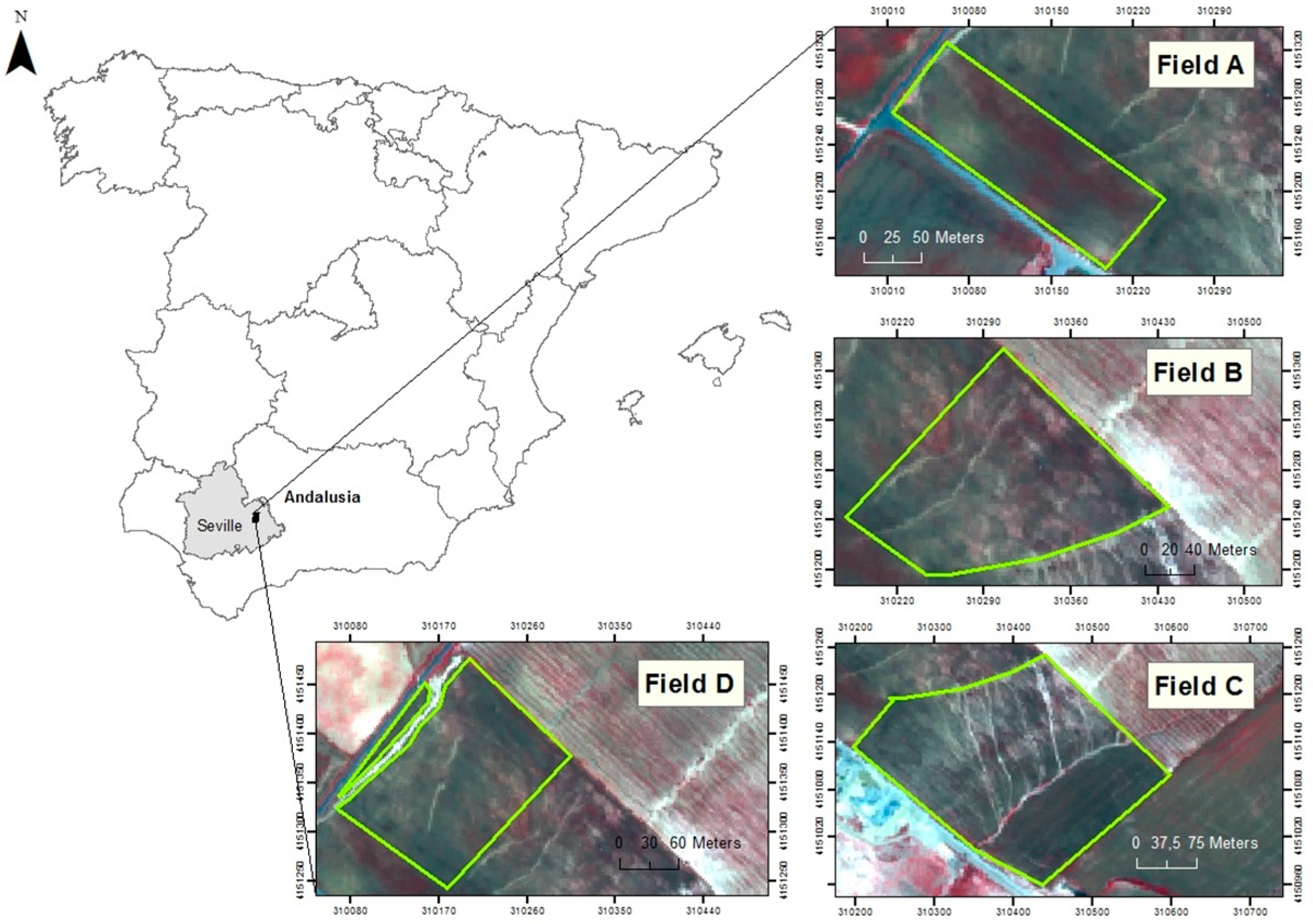
2.1. Study Area, Remote Imagery, and Discrimination of Wild Oat Patches in Wheat Fields

This study was conducted in 2006 and 2008 in four winter wheat fields named A, B, C, and D, located near La Lantejuela (a province of Seville, Andalusia, southern Spain) (Figure 1). This region is representative of Andalusian dryland crops, with a typical continental Mediterranean climate, a relatively flat relief, and an average height of 380 m above sea level. During 2007, the four wheat fields were sown with sunflower, following the typical crop rotation of this agricultural region. Wild oat infestations were not recorded during 2007 as expected because summer crops are usually free of this weed species. Two QuickBird multispectral satellite images were acquired on 10 May 2006 (scene of 47 km²), and 22 May 2008 (scene of 73 km²), which corresponds to spring in the experimental conditions. Wheat crops were in the initial senescence stage and the wild oat weed patches were at the advanced seed maturation stage. These phenological stages were described as the best moment for a successful discrimination of wild oat in wheat fields by [11,19]. Although 11 and 15 wheat fields were present in the entire QuickBird images, the four wheat fields were selected because they matched in both imagery, which was essential for studying the persistence in the location of wild oat patches. Because the location of the study was in a farmer-managed area and the farmers make decisions individually, we found that the rest of the 2006 wheat fields had been changed to olive orchards during the field survey developed in 2008 (more details in [12]). The total area of fields A, B, C, and D was 1.74, 2.52, 6.34, and 2.77 ha, respectively.

Although a number of pixel- and object-based (OBIA) classifications with different algorithms were evaluated to accurately map the wild oat infestation distribution, the most accurate maps (classifications higher than 97%) for the four fields both years were obtained by using OBIA and support vector machine classification algorithm. As consequence, the maps generated by using these procedures were employed in the present study. More detailed characteristics of remote imagery, image processing and the performance of algorithms to distinguish wild oat from wheat in the four studied fields are described in [12].

2.2. Spatial Persistence of Wild Oat Patches in Wheat Fields

To determine the spatial persistence of the wild oat patches in each wheat field, three different tests were conducted to evaluate if the wild oat patches were persistent in location from 2006 to 2008 and to identify if new weed patches (2008) were connected or influenced by the older patches (2006).

2.2.1. Change Detection Test

A statistical change detection analysis between 2006 and 2008 QuickBird imagery was conducted in each of the four wheat fields to identify and quantify the differences in land use (infested wheat/weed-free wheat) at the two studied dates. The analysis was based on the measurement of the area classified as wild oat and wheat in both years. Using the weed and crop distribution of the 2006 imagery as the initial reference state, a comparison of the land use of each pixel in that initial and final state (2008) was made. Three scenarios were studied: No change, when the land use of a pixel remained the same (wheat–wheat or wild oat–wild oat) in 2006 and 2008; Wheat increase, when a pixel in 2006 was classified as wild oat, whereas in 2008 it was classified as wheat; and wild oat increase, when a pixel in 2006 was classified as wheat and as wild oat in 2008.

2.2.2. Spatial Autocorrelation Test

To determine the spatial distribution, a spatial autocorrelation test of the wild oat pixels for each wheat field in both years (2006 and 2008) was developed by considering that an aggregation of weed pixels would indicate that the infestations will spread in patches and facilitate the design of maps for SSWM in the subsequent years. The analysis of these spatially located data was performed by Moran’s Index (Moran’s I) [20]. The Moran’s I is a measure of the spatial autocorrelation that presents the studied variable (wild oat) in the field. The spatial autocorrelation is based on the first law of geography that everything is related to everything else, but near things are more related than distant things [21]. Moran’s I is applied to points that have continuous variables associated with their intensities. These statistics are used to compare the value of the variable xi in one location with the value at all other locations xj. It is formally defined by Equation (1):

$$\mathrm{I}=\frac{n{{\displaystyle \sum }}_{i=1}^n{{\displaystyle \sum }}_{j=1}^n{w}_{ij}(x_i-\overline{x})(x_j-\overline{x})}{{{\displaystyle \sum }}_{i=1}^n{{\displaystyle \sum }}_{j=1}^n{w}_{ij}{{\displaystyle \sum }}_{i=1}^n{(x_i-\overline{x})}^2}$$

(1)

where n is the number of cases in the analysis, x_i and x_j are the variable values at locations i and j (i ≠ j), $\overline{x}$ is the mean of the pixel value of the referenced points and w_ij is a distance-based weight, which is the inverse distance between i and j (i.e., w_ij = 1/d_ij). The spatial resolution of the Moran’s I was 2.4 m, equal to that of the satellite image.

The values of global Moran’s I usually ranges from −1 to 1, although the values can exceed both limits [22]. Positive values (values higher than 0) indicate a positive spatial autocorrelation and a clustering or aggregation tendency, whereas negative values (values lower than 0) suggest negative spatial autocorrelation and a geographical dispersion. A value of 0 indicates perfect spatial randomness and no correlation.

2.2.3. Spreading Distance Test

To determine if the new wild oat patches detected in 2008 could be influenced by the spatial distribution of the initial patches detected in 2006, a spreading distance analysis was conducted [23]. In this analysis and for each studied field, the distance between each pixel classified as wild oat in the 2008 image and in all directions nearest the pixel classified as wild oat in the 2006 image, including the same overlapped pixel (zero distance), was calculated while considering that the latter could be the source of the seed. Once the minimum distances between wild oat pixels in both years were calculated, this information was represented in a frequency histogram to evaluate whether the distribution of the wild oat pixels observed in 2008 tended or not to be close to the wild oat pixels in 2006. This method was an adaptation from [17].

A frequency distribution close to the origin could suggest a great spatial dependency from the 2008 patches to the 2006 ones, i.e., a short distance for spreading of the seed from the weed source (wild oat present in 2006). Nevertheless, a frequency distribution distant from the origin could indicate a higher distance for spreading and great influence of external factors such as wind or agricultural machinery. Finally, a distribution with several peaks along the studied distance and without tendency could suggest a random allocation of weeds and that no dependence between the wild oat patches emerged in both years could be established. The closer to the origin the distribution is, the more the spatial aggregation of weeds can be observed. This information would be an excellent tool to assist with understanding the persistence in the location of this weed, to explore its behavior and to decide on an early SSWM strategy in subsequent years.

The spatial persistence study of wild oat patches in wheat fields was conducted by the ArcGIS 10.3 software (ESRI, 2015, Redlands, CA, USA).

2.3. Maps for Site-Specific Weed Management (SSWM) Simulations

The surfaces covered by wild oat and wheat in the four fields studied in 2006 and 2008 were obtained by Castillejo-González et al. [12] in an earlier study, as previously mentioned in Section 2.1. To obtain these maps, the density of the weed infestation was not considered. Nevertheless, according to Barroso et al. [24], only the weed patches with moderate or high infestation density (more than 10 panicles per m²) must be treated. Considering that the spatial resolution of the QuickBird images used to obtain the wild oat patches distribution was 2.4 m (5.76 m²/pixel), low density wild oat infestations could be practically undetectable with this spatial resolution. For this reason, all the pixels classified as wild oat will be considered to present an infestation level high enough to be treated.

With the aim of building site-specific herbicide treatment maps, the whole surface of the four wheat fields was overlapped by a homogeneous grid. The design of the grid is user-configurable. For example, in this investigation and according to the weed control spraying described in [25], the characteristics of the wheat and weed-control spraying machinery showed a grid size of 0.5 × 0.5 m. Each field was then divided into treatment units (TU) of 0.5 × 0.5 m, which were classified as infested or not infested according to the level of wild oat present in each TU. According to Barroso et al. [26], all of the TUs that presented less than 25% of infested area (low infestation level) were not considered to be treated.

The weed infestation data used in the design of the SSWM were obtained considering 2006 as the origin of the infestation, and predicting different scenarios of weed emergence for the next wheat crop (2008) to be treated. Four different herbicide treatments were simulated based on the results obtained in the dispersal distance study (see Section 3.1.3). The first simulation planned the SSWM only for the wild oat infestations observed in the 2006 image (origin). The other simulations were obtained considering that the area infested next year will be higher than the original infestation and that this increase will be connected with the spreading distance of the wild oat. Thus, three new simulations were established with an increase of 25%, 50%, and 75% of the average spread distance of the four fields jointly from the origin of wild oat infestation.

2.4. Economic Analysis

The SSWM simulated herbicide treatments in the previous section were used to calculate their economic profitability. Although Barroso et al. [17] previously recommended a buffer of 4 m around the wild oat patches observed in one year to construct the treatment maps for the following year, five weed management simulations including more buffer distances were conducted in the four wheat fields by considering: (1) an overall application (S_OT); (2) only the weed patches observed in the 2006 image (S_0m); (3) a 1-meter buffer around the 2006 weed patches (S_1m); (4) a 4-meter buffer around the 2006 weed patches (S_4m); and (5) a 9-meter buffer around the 2006 weed patches (S_9m). S_OT did not require the use of precision agriculture and fits with the normal choice of farmers who usually prefer to treat weed-free or low-infested areas rather than assume the risk of allowing weeds to go untreated [27], whereas simulations S_0m, S_1m, S_4m, and S_9m did require the use of SSWM and precision agriculture techniques. The high cost of the SSWM technology usually involves a large farm size to ensure the amortization of the cost, or requires cooperation between several farms [28]. Therefore, the economic study presented herein was developed by considering the four fields together under the hypothesis that farmers collaborate with their colleagues and share precision agriculture equipment.

The economic profitability for each weed control strategy was performed with the calculation of the net returns, adapted from Gómez-Candón et al. [29], according to Equation (2):

$$NR=(\widehat{y}{{\displaystyle \sum }}_{i=1}^n(WOFA+WOTA)+(\widehat{y}-L){{\displaystyle \sum }}_{i=1}^{n}WONTA)p-(C_s+C_a+H{{\displaystyle \sum }}_{i=1}^{n}WOTA+C_o)$$

(2)

where NR is the net return in € ha⁻¹; n is total number of 0.5 × 0.5 m treatment units (TU); i is the TU number; $\widehat{y}$ is the considered weed-free wheat yield in kg ha⁻¹; L is the yield loss estimated in each infested TU with no herbicide application in kg ha⁻¹; WOFA_i is the A. sterilis-free area of each TU in ha; WOTA_i is the A. sterilis-infested herbicide-treated area of each TU in ha; WONTA_i is the A. sterilis-infested untreated area of each TU in ha; p is the price of wheat grain (0.30 € kg⁻¹); C_s is the cost of acquiring and processing the images (only considered in site-specific treatments: 10 € ha⁻¹); and C_a is the treatment cost with a sprayer (6.6 € ha⁻¹ for spraying with a standard sprayer and 11 € ha⁻¹ for precision application); H is the specific herbicide cost (40 € ha⁻¹). In this study, glyphosate was applied at pre-emergence, and C_o includes all of the other costs involved in production such as tillage, seed, fertilizers, and harvest (300 € ha⁻¹). All these values are according to current prices and costs for a standard farm in southern Spain in 2017.

In addition, and to assess different levels of productivity, four agronomic scenarios that consider the potential yield of wheat in Spain and the productivity loss due to wild oat were also analyzed to test the SSWM strategies. Considering that the potential average wheat yield in Spain ranges from 1500 to 4500 kg ha⁻¹ and that the productivity loss due to wild oat infestation varies between 100 and 400 kg ha⁻¹ [30], the following four combinations based on wheat yield (first value) and wild oat loss (second value) were established: (1) 4500 and 100 kg ha⁻¹; (2) 4500 and 400 kg ha⁻¹; (3) 1500 and 100 kg ha⁻¹; and (4) 1500 and 400 kg ha⁻¹. Scenarios #1 and #4 represent the highest and the lowest productive possibilities, respectively.

All the spatial data procedures to obtain the wild oat maps for the design of site-specific treatments were conducted using ArcGIS 10.3 (ESRI, Redlands, CA, USA), whereas the economic analyses based on these maps were performed using Microsoft Excel (Microsoft, 2013, Redmond, WA, USA).

3. Results

3.1. Spatial Persistence of Wild Oat Patches in Wheat Fields

3.1.1. Change Detection

The spatial distribution of the change detection analysis shows the wheat-wild oat classifications obtained from the 2006 and 2008 imagery (yellow‒green fields) and the change detection analysis comparing the land use of each pixel in both years (red‒blue‒gray fields) (Figure 2). The temporal trend observed in the distribution of wild oat in the wheat fields showed a generalized increase in the weed area (red), although some infested areas in 2006 that changed to weed-free wheat in 2008 (blue) can also be observed. Field B displayed the clearest increase of wild oat infestation in the subsequent year, with an important area of weed-free wheat in 2006 that changed to wild oat infestation in 2008 and an insignificant area classified as wild oat in 2006 that was not infested in 2008. The other fields that were studied showed different proportions of wild oat and wheat increase, especially in fields C and A, where some areas of previous weed infestations in 2006 disappeared in 2008, which was probably due to the management of the farmer.

The change detection analysis displays the evolution and the change area of the weed patches, exhibiting the percentage of the area that maintained the same land use in both years and the area that changed from wheat to wild oat or vice versa (

Table 1. Crop-weed area change comparison between 2006 and 2008 in the four wheat fields.

Area 1	Field A			Field B			Field C			Field D
	WO06 2	W06	T08	WO06	W06	T08	WO06	W06	T08	WO06	W06	T08
WO08	0.37	0.45	0.82	0.68	0.83	1.51	0.98	0.84	1.82	0.62	0.48	1.10
W08	0.31	0.61	0.92	0.05	0.96	1.01	1.21	3.35	4.56	0.30	1.37	1.67
W06	0.68	1.06	1.74	0.73	1.79	2.52	2.19	4.19	6.38	0.92	1.85	2.77

¹ Values: surface occupied for each land use in hectares; ² Land uses: WO for Wild Oat; W for Wheat; T for Total (WO + W). Year of study: 06 for 2006; 08 for 2008

). For example, in 2006, field A showed 0.68 ha infested with wild oat, but only 0.37 ha of this infestation remained in 2008 because the other 0.31 ha changed to weed-free wheat. Nevertheless, the total area infested with wild oat in 2008 was 0.82 ha because 0.45 ha classified as wheat in the 2006 imagery were infested with wild oat in 2008. Fields B, A and D showed an increase in the weed area between the two years studied of 31% (from 0.73 ha to 1.51 ha), 8% (from 0.68 ha to 0.82 ha) and 6.5% (from 0.92 ha to 1.10 ha), respectively. Field C showed an opposed evolution of weeds, with a decrease of wild oat surface close to 6% (from 2.19 ha in 2006 to 1.82 ha in 2008).

Considering the total area classified as wild oat in 2006, the spatial persistence, that is, the proportion of area that maintained the same land use in 2008, was highly variable among the fields. Field B exhibited the highest persistence, with 93.2% of the wild oat area in 2006 (0.68 ha of the 0.73 ha infested in 2006) showing the same location in 2008. Fields D and A showed a medium-high wild oat persistence, with 67.4% (0.62 ha of 0.92 ha infested in 2006) and 54.4% (0.37 ha of 0.68 ha infested in 2006) of unchanged weed area, respectively. Finally, field C maintained only 44.8% (0.98 ha of 2.19 ha infested in 2006) of the weed area in 2008, which indicated a change of more than half of the wild oat area in 2006 to wheat in 2008. The wheat persistence showed a slightly more homogeneous behavior. Fields C and D conserved the highest weed-free wheat areas without a land use change with 80% (3.35 ha of 4.19 ha of the wheat in 2006) and 74.1% (1.37 ha of 1.85 ha of the wheat in 2006), respectively. A lower wheat persistence could be observed in fields A and B, where only 57.5% and 53.6% (0.61 ha of 1.06 ha and 0.96 ha of 1.79 ha), respectively, of wheat classified in 2006 maintained the same land use.

3.1.2. Spatial Autocorrelation

The wild oat persistence observed from the change detection study was evaluated by a spatial autocorrelation analysis performed by Moran’s Index (

Table 2. Spatial autocorrelation analysis in the four fields studied during 2006 and 2008.

		Moran Index 1
Field A	2006	0.67
	2008	0.82
Field B	2006	0.76
	2008	0.83
Field C	2006	0.84
	2008	0.60
Field D	2006	0.76
	2008	0.70

¹ Confidence level 99%.

). The autocorrelation values obtained from the four fields studied for both years (2006 and 2008) revealed that all the fields showed a noticeable positive spatial autocorrelation, which indicates a high level of wild oat aggregation, with Moran’s I values ranging from 0.60 to 0.84. Field B showed the highest positive autocorrelation values with a Moran’s I of 0.76 and 0.83 in 2006 and 2008, respectively, whereas field D showed the lowest Moran’s I results with values of 0.76 and 0.70 in 2006 and 2008, respectively. Nevertheless, field C displayed the most extreme spatial autocorrelation values, with a significant weed aggregation in 2006 (Moran’s I of 0.84) and a more moderate level of aggregation in 2008 (Moran’s I of 0.60).

3.1.3. Dispersal Distance

For the four studied fields, the spreading distance analysis showed that the new emergence of wild oat observed in 2008 was clearly influenced by the wild oat patches that already existed in 2006 (Figure 3). Considering the differences in size and shape of the fields and the amount of new wild oat patches that emerged from each field, the maximum spreading distances of these fields significantly varied. The frequency histograms showed a clear decreasing trend in which the new weeds of 2008 tend to emerge close to the weeds of 2006. All the fields showed that 25% of the newly emerged wild oat of 2008 was located in the closest 2 m around the weeds identified in 2006, except for field C, where the same proportion of new wild oat was spread around 2–3 m of the previous patches of 2006. This spreading distance was less uniform as the percentage of the weeds increased. For instance, 50% of new wild oat was found within 2–3 m of the 2006 weeds in field A, 3–4 m in field D, 5 m in field B, and 7–8 m in field C. In the same way, 75% of the new weeds were found at 5 m, 8 m, 12 m and 20 m from the source in fields A, D, B and C, respectively. Finally, although the maximum spread distances were considerably higher in most of the fields, most of the new wild oat patches (95%) were observed at 10 m, 18 m, 27 m and 33 m from the source in fields A, D, B and C, respectively.

3.2. Maps for Site-Specific Weed Management (SSWM)

To obtain the average behavior of the studied fields, a unique cumulative frequency histogram jointly considering the data of the four fields was calculated (Figure 4). The cumulative frequency histogram showed an exponential distribution where 25%, 50% and 75% of the new weeds that emerged in 2008, which would correspond to 1 m, 4 m, and 9 m from the origin, respectively. From this point, there was a decrease of the slope of the curve, ending in a plateau where a small increment of the percentage of new wild oat patches was distributed along large distances. We used the information obtained in the cumulative frequency histogram to design the four simulated SSWM treatments (S_0m, S_1m, S_4m and S_9m) established in Section 2.4. An increase in the area of 0 m, 1 m, 4 m, and 9 m around the 2006 weeds was designed in the treatments considering an increase of the spreading distance from the weed source of 0%, 25%, 50% and 75% regarding the new weeds emerged in 2008, respectively.

Table 3. Comparison of the treated areas considering simulations form S_0m to S_9m in the four wheat fields.

	Field A				Field B				Field C				Field D
	S0m 1	S1m	S4m	S9m	S0m	S1m	S4m	S9m	S0m	S1m	S4m	S9m	S0m	S1m	S4m	S9m
WOA 2	39.08	51.72	74.91	89.59	29.08	34.80	47.56	60.71	34.27	39.68	51.29	63.93	33.30	41.54	58.79	75.41
TA	40.45	52.87	75.60	90.05	29.68	35.40	47.95	60.99	34.61	39.99	51.35	63.86	34.09	42.34	59.26	75.74
WOTA	99.26	99.67	99.77	100	99.45	99.66	99.92	99.93	98.99	99.21	99.30	99.34	99.02	99.48	99.69	99.81
WOTA08	44.49	59.56	84.80	96.57	45.68	53.86	70.23	82.31	53.83	59.85	71.81	82.46	57.13	67.30	83.11	92.82
WOFTA08	17.33	22.74	33.13	42.03	1.51	2.10	4.35	9.35	17.25	20.65	28.01	36.94	9.69	13.47	23.30	35.20

¹ Sx: simulation areas considering buffers ranging from 0–9 m regarding 2006 weed infestation; ² WOA: % of Wild Oat-infested Area considering simulation x (S_x); TA: % of Treated Area; WOTA: % of Wild Oat-infested Treated Area; WOTA₀₈: % of Wild Oat-infested Treated Area considering 2008 imagery infestation; WOFTA₀₈: % of Wild Oat Free Treated Area considering 2008 imagery infestation.

shows a comparison between the concordance of the SSWM treatments designed for the simulated (S_0m, S_1m, S_4m and S_9m) weed-infested areas and their level of wild oat control over the real wild-oat infestations observed in 2008 for each field. Simulation S_0m considered an initial weed infestation similar to that classified in 2006 imagery and showed a close level of infestation (WOA) among the fields with values that ranged from 29% in field B to 39% in field A. When the study attempted to predict the growth of wild oat, S_1m, S_4m and S_9m, the initial spatial distribution of the weeds and the shape of the plot offered a different behavior in the predictions. Fields B and C moderately increased the infested surface with approximately 30% more weed infestation areas in S_9m regarding the initial simulation (S_0m), which showed 60.71% in S_9m and 63.93% of WOA, respectively. Field D exhibited a higher increase of infestation levels than fields B and C and was covered with wild oat of S_9m at 75.41% of the field area, which represented 42% more surface in S_9m than S_0m. Finally, field A presented the highest infestation levels in all the simulations with more than 50% of new weeds in S_9m in relation with S_0m, which implies a wild oat cover of almost 90% of the entire field surface.

Independent of this different behavior, the percentage of wild oat-infested treated area of the treatments proposed (WOTA) was similar in all of the simulations and fields analyzed with values higher than 99%. In addition to this high coincidence of WOTA in all studied fields, the maximum difference between the treated area (TA) and the simulated infested area (WOA) did not exceed 1.5% in any simulation, which indicates that treated areas without weed infestations or with infestation levels lower than 25% in the treatment unit area were minimal.

Finally, when comparing the weed location predicted from the 2006 imagery with the current weed infestation in 2008 (WOTA₀₈), the results showed an increasing trend of the infested area overlapped until more than 80% when treated with S_9m. The overlaps between the actual 2008 weed infestation and the 2006 predicted simulations varied according to the spatial distribution of the wild oat patches. Fields A and D obtained more than 90% of the coincidence between the simulated treated in S_9m and the 2008 real wild oat infestation (WOTA₀₈), with values that reached 96.57% and 92.82%, respectively. In this case, field A showed a more progressive increase because its efficiency in S_0m was the lowest with a value of 44.49%. However, fields B and C had lower percentages of 2008 infested area treated in simulation S_9m with values of 82.31% and 82.46%, respectively, although field C showed the second highest WOTA₀₈ value in S_0m with an efficacy of 53.83%. In general, the lowest overlap of predicted‒actual wild oat infestations was observed in field B, whereas fields D and A showed the maximum overlap.

Additionally, the wild oat free areas treated with these simulations were analyzed in order to determine the unnecessarily treated areas (WOFTA₀₈). Field B showed the lowest WOFTA₀₈ value with a maximum of 9.35% of overtreated area. Nevertheless, the level of the unnecessarily treated area in fields A, C and D were higher with values that ranged from 9.69%, in field D with the S_0m simulation, to 42.03%, in field A with the S_9m simulation. In all simulations for all fields analyzed, the wild oat free areas treated were smaller than those observed with the standard overall treatment, which offered a 53.08%, 40.01%, 71.56% and 60.24% of unnecessary treated area for fields A, B C and D, respectively (data not shown).

Figure 5 depicts the initial wild oat infestation in the 2006 imagery and the proposed treatments of the different simulations in the four fields studied. The S_0m and S_1m simulations offered a treatment pattern that was very similar to the initial weed infestation in all of the fields. Nevertheless, as the buffer distances rose in S_4m and S_9m, the increase in the treated surface was considerable. This considerable increment can be mainly observed in field A, where the treated area covered more than 75% in simulation S_4m and covered more than 90% in S_9m. Therefore, the treated area proposed clearly depended on the initial spatial distribution of the wild oat patches and on the dimensions and shapes of the fields.

3.3. Economic Analysis

The economic analysis shows the net return (€ ha⁻¹) for each herbicide application simulated for the four agronomic scenarios analyzed according to variations of the wheat yields and losses due to wild oat (

Table 4. Economic net returns and profits as a result of simulated herbicide application strategies considering different agronomic scenarios.

	Scenario #1: Expected Yield 4500 kg ha−1; Yield Losses Due to Wild Oat 100 kg ha−1
	Field A		Field B		Field C		Field D		Fields A + B + C + D
	NR1	Profit2	NR	Profit	NR	Profit	NR	Profit	NR	Profit
SOT 3	1003	100.0	1003	100.0	1003	100.0	1003	100.0	1003	100.0
S0m	1005	100.2	1007	100.4	1011	100.8	992	98.9	1006	100.2
S1m	1002	99.9	1007	100.3	1010	100.6	988	98.5	1004	100.0
S4m	997	99.3	1004	100.1	1006	100.3	980	97.6	999	99.6
S9m	993	98.9	1001	99.8	1002	99.9	969	96.6	994	99.1
	Scenario #2: Expected Yield 4500 kg ha−1; Yield Losses Due to Wild Oat 400 kg ha−1
	Field A		Field B		Field C		Field D		Fields A + B + C + D
	NR	Profit	NR	Profit	NR	Profit	NR	Profit	NR	Profit
SOT	1003	100.0	1003	100.0	1003	100.0	1003	100.0	1003	100.0
S0m	982	97.8	978	97.5	999	99.6	977	97.3	988	98.5
S1m	985	98.2	982	97.8	999	99.6	977	97.3	989	98.6
S4m	990	98.7	988	98.5	999	99.5	974	97.0	991	98.7
S9m	991	98.8	992	98.9	997	99.4	967	96.4	989	98.6
	Scenario #3: Expected Yield 1500 kg ha−1; Yield Losses Due to Wild Oat 100 kg ha−1
	Field A		Field B		Field C		Field D		Fields A + B + C + D
	NR	Profit	NR	Profit	NR	Profit	NR	Profit	NR	Profit
SOT	103	100.0	103	100.0	103	100.0	103	100.0	103	100.0
S0m	105	101.6	107	103.8	111	107.6	92	89.0	106	102.2
S1m	102	98.8	107	103.0	110	106.0	88	85.4	104	100.2
S4m	97	93.5	104	101.0	106	102.6	80	77.1	99	95.8
S9m	93	89.5	101	98.1	102	98.6	69	67.1	94	90.8
	Scenario #4: Expected Yield 1500 kg ha−1; Yield Losses Due to Wild Oat 400 kg ha−1
	Field A		Field B		Field C		Field D		Fields A + B + C + D
	NR	Profit	NR	Profit	NR	Profit	NR	Profit	NR	Profit
SOT	103	100.0	103	100.0	103	100.0	103	100.0	103	100.0
S0m	82	78.9	78	75.4	99	96.2	77	74.2	88	85.5
S1m	85	82.2	82	78.9	99	96.1	77	74.1	89	86.5
S4m	90	87.3	88	85.5	99	95.6	74	71.2	91	87.6
S9m	91	88.1	92	88.9	97	94.3	67	64.6	89	86.3

¹ NR: Net economic Return (€/ha); ² Profit: percentage of benefit (%) obtained in each simulation considering S_OT the earnings base (100%); ³ Simulations: S_OT standard overall treatment in the wheat fields; S_0m, S_1m, S_4m and S_9m: treatment of ≥25% of wild oat infested pixels considering buffers ranging from 0–9 m regarding 2006 weed infestation.

). For an easier comparison, the net return was complemented with a profit value and a percentage of benefit obtained in each simulation considering the standard overall treatment as the earning base (100%). The economic analysis was conducted for the four fields independently, and to obtain the average behavior of the studied fields, the same analysis was calculated by jointly considering the data of the four fields.

The results suggest that the most profitable strategy was highly dependent on the agronomic conditions. Regardless of the expected yield, when the yield loss due to wild oat was at a minimum (scenarios #1 and #3: 100 kg ha⁻¹), some SSWM treatments could be more competitive than the overall treatment (S_OT). In scenario #1 and for simulations S_0m, S_1m and S_4m, fields B and C offered profits values higher than 100%. For simulations S_0m, S_1m and S_4m, the benefits were higher in scenario #3, where field B and C obtained profit values until almost 104% and 108%, respectively. However, fields A and D showed benefit values lower than the overall treatments (S_OT) in all of the simulations, except field A in simulation S_0m, which reached values slightly superior to 100%. Different behavior can be observed when the yield losses due to wild oat were at a maximum (scenarios #2 and #4: 400 kg ha⁻¹) and considering that all SSWM simulations offer profit values lower than 100% for both scenarios and every yield independently and for the average of the four fields.

Considering the increasing of the buffer distance in the simulations (S_0m, S_1m, S_4m and S_9m), the profit percentages generally decreased as the buffer distance increased, being more distinguished when expected yields were low (scenarios #1 and #3). Nevertheless, in fields A and B, when there were maximum yield losses due to wild oat (scenarios #2 and #4), an increase of the profits could be observed as the buffer distance increased.

Analyzing the average value of all the fields jointly (fields A + B + C + D), only simulations S_0m and S_1m exceeded the earning base of 100% when the yield loss due to wild oat was at a minimum (scenarios #1 and #3), showing a decreasing trend of profits in all simulations. This trend was not so clear when the yield losses due to wild oat were at a maximum (scenarios #2 and #4), and almost the same profit values in all the SSWM simulations can be observed. Finally, simulation S_9m tended to show lower profit values than the overall application in all the scenarios, which was more obvious as the wheat yield decreased and the yield loss due to weed presence increased.

4. Discussion

The statistical change detection analysis between 2006 and 2008 imagery showed that all fields except field A suffered moderate-remarkable infestation increases in 2008, which is expected in conventional systems with diverse annual crops (wheat-sunflower in that area) and without fallow rotation [31]. The reasons for the differences between fields would be related to the usual high variability inherent to studies conducted under field conditions. For example, the size and shape of weed patches vary within the field and according to every species [32,33,34] or the field management practices [35,36], among others. Other works about multi-temporal spatial distribution of weed patches related the differences in their field experiments with the remaining propagule bank, the presence of favorable conditions (soil moisture and nutrient) and the usual short distance of seed dispersal [37]. Numerous experiments regarding particularly the wild oat patch dynamics or changes in wild oat patches between sites have shown that different efficacy of the herbicide applications under diverse environmental conditions between years, seed movement into the field from neighboring sites due to natural dissemination or agricultural operations, or significant different of chemical and physical soil properties between sites even located very close some of others are key factors for understanding its spatial persistence [2,17,38].

In our study, the increases of the infestation level in the 2008 wheat crops were probably due to inappropriate farm management with no specific wild oat herbicide treatments or with sprayings in an incorrect period of weed growth. That situation can be observed in field A, where the numeric results showed an increase of the wild oat-infested area, whereas the spatial analysis allowed displaying the increase of the weed area in the majority of the field surface except in some edges of the field A, where a reduction of the infestation comparing to the observed in 2006 was detected. This reduction may also be due to the correct wild oat management of the adjacent field that affected the closest area of field A. In addition, the spatial pattern measure of the infestation showed a high positive spatial autocorrelation in all the fields and years analyzed, which suggests an aggregation tendency of weed growth in the patches. González-Andújar et al. [39] obtained similar results when analyzing the aggregation of A. sterilis.

Regarding the average dispersal distance, our study showed that 75% of the new wild oat patches tend to be in a 9-m buffer around old foci, but it is possible to find new wild oat infestation up to 25 m. A detailed study of the dispersal of wild oat patches by Barroso et al. [17] indicated that new patches caused by wind and by agricultural machinery rarely exceeds 3 m and that an annual patch displacement of 2–3 m in the tillage direction was observed, although isolated plants could be located up to 30 m from the original sources. One of the conclusions they came to is that this spatiotemporal distribution permits prediction of future infestation behavior and helps us to design SSWM treatments in subsequent years to reduce herbicide use by only treating infested areas. In our study, when treatments were based on predicted weed maps based on 2006 infestations (simulations S_0m, S_1m, S_4m and S_9m), herbicide treatment simulations in real 2008 infestations were significantly reduced compared to overall treatments. As an example, considering the recommendation by Barroso et al. [17] of a buffer of 4 m around patches to construct the treatment maps for the following year, Table 3 shows that our simulations (S_4m) controlled 70.23% to 84.80% of wild oat in the different fields (WOTA₀₈), with a range of 4.35% to 33.13% of wild-oat-free treated area (WOFTA₀₈).

From an ecological point of view, the unnecessary wild-oat-free areas treated with any of our simulations were smaller than those observed with an overall treatment. From an economic point of view and according to our simulations, the best management strategies were dependent on the agronomic conditions of the fields and on the percentage of infestation observed in each field. For example, considering the highest yield losses due to wild oat (400 kg ha⁻¹), the profits increased as the expected wheat yield was higher (scenarios # 2 and 4). Similar conclusions were obtained by Ruiz et al. [38], who reported that site-specific treatments were advantageous mainly in high-returns systems. In our study, field C showed a higher profitability in all the scenarios probably due to patch distribution was concentrated, e.g., new 2008 patches covering almost the same total infested area than in 2006. Similarly, as Barroso et al. [26] showed in experimental studies conducted in winter barley crops under Spanish conditions, the number and size of infested patches in a field has a great influence on the economic analysis, increasing the profits as the infestation area was concentrated in a few large patches. For most of the analyses presented herein, the site-specific application for the weed infestation observed in the 2006 image (S_0m) resulted in higher profits regarding the overall application (S_OT) when the yield losses due to wild oat were minimal (100 kg ha⁻¹), and even the 1-meter buffer around the 2006 wild oat infestation (S_1m) and the 4-meter buffer around the 2006 weed infestation (S_4m) were more competitive than SOT in some fields. Concerning the maximum yield losses due to weeds (400 kg ha⁻¹), all the SSWM simulations were less competitive than the overall treatments in all the fields analyzed, being this difference more remarkable when the expected wheat yield was at a minimum (scenario #4). The profitability of SSWM is highly dependent on the characteristics of the study: yield levels, herbicide price and technology available. Modification of those parameters, such as the width of the boom sprayer, can modify the results. For that reason, the economic analysis proposed is customizable and provides objective results in the context of SSWM.

Although the profit variations achieved between SSWM and the overall treatments were slight and net returns are not always guaranteed, our recommendation would be to persuade farmers to adopt SSWM. The main reason is that one of the bases of this control approach is to provide a framework of weed spatial information to make rational use of herbicides by adjusting it according to the actual needs or applying other strategies such as the use of plant derivatives with allelopathy effect (natural herbicides) to reduce the chemical pollution [40,41] for the better protection of the environment and for a consumer perspective. Our findings are in agreement with previous studies [2,42,43,44]. They reported that even when the direct economic benefit for farmers seems to be modest and could be questionable in some scenarios, a reduced (often very expensive) herbicide treatment strategy based on weed coverage was favorable from the consumer and environmental safety point of view, providing a net surplus to the society due to the high potential for the decrease of herbicide input. The SSWM is applicable even in fields with high infestation levels because some field areas do not require any herbicide treatment. As stated before, this view also fits with the current European legislation and research concerns [3], which support practical solutions for a sustainable use of pesticides and the use of the most advanced and latest technologies. Our results have economic, agronomic, and environmental implications and offer opportunities to extrapolate them to other areas worldwide where wild oat, one of the most harmful and competitive weeds in winter cereals, causes relevant yield losses.

5. Conclusions

The results of the present study show that the spatial wild oat patch persistence and dynamics in wheat fields for the Spanish conditions evaluated were highly dependent on previous infestations, which permitted the prediction of future infestation behaviors to design SSWM treatments in subsequent years and to spray only infested areas. The data obtained showed that the best management strategies are dependent on the agronomic conditions (e.g., expected wheat yield) and the percentage of infestation observed in each field. Although the economic profit variations between SSWM and the overall treatments achieved were slight and there were no relevant differences in net returns in some scenarios in comparison with overall applications, site-specific treatments are preferred to control wild oat for a lower herbicide use and a reduction of potential environmental pollution. This reduction in herbicide input is safer from a consumer and ecological point of view and fits with the current European legislation.

References

1. Fernández-Quintanilla, C.; Navarrete, L.; Torner, C.; Sánchez Del Arco, M.J. Avena sterilis en cultivos de cereales. In Biología de las Malas Hierbas de España; Sans, F.X., Fernández-Quintanilla, C., Eds.; MV-Phytoma España: Valencia, Spain, 1997; pp. 4–17. [Google Scholar]
2. Barroso, J.; Fernández-Quintanilla, C.; Ruiz, D.; Hernaiz, P.; Rew, L.J. Spatial stability of Avena sterilis spp. ludoviciana populations under annual applications of low rates of imazamethabenz. Weed Res. 2004, 44, 178–186. [Google Scholar] [CrossRef]
3. Horizon 2020. Available online: http://ec.europa.eu/programmes/horizon2020 (accessed on 12 December 2018).
4. Regulation (EC) 1107/2009. Available online: http://eur-lex.europa.eu/legal-content/EN/TXT/?qid=1494242522151&uri=CELEX:32009R1107 (accessed on 12 December 2018).
5. Directive 2009/128/EC. Available online: http://eur-lex.europa.eu/legal-content/EN/TXT/?qid=1494246385637&uri=CELEX:32009L0128 (accessed on 12 December 2018).
6. López-Granados, F. Weed detection for site-specific weed management: Mapping and real-time approaches. Weed Res. 2011, 51, 1–11. [Google Scholar] [CrossRef]
7. De Castro, A.I.; Jurado-Expósito, M.; Peña-Barragán, J.M.; López-Granados, F. Airborne multi-spectral imagery for mapping cruciferous weeds in cereal and legume crops. Precis. Agric. 2012, 13, 302–321. [Google Scholar] [CrossRef]
8. De Castro, A.I.; López-Granados, F.; Jurado-Expósito, M. Broad-scale cruciferous weed patch classification in winter wheat using QuickBird imagery for in-season site-specific control. Precis. Agric. 2013, 14, 392–413. [Google Scholar] [CrossRef] [Green Version]
9. Peña-Barragán, J.M.; López-Granados, F.; Jurado-Expósito, M.; García-Torres, L. Spectral discrimination of Ridolfia segetum and sunflower as affected by phenological stage. Weed Res. 2006, 46, 10–21. [Google Scholar] [CrossRef]
10. López-Granados, F.; Peña-Barragán, J.M.; Jurado-Expósito, M.; García-Torres, L. Using remote sensing for identification of late-season grass weeds patches in wheat (Triticum aestivum L.) for precision agriculture. Weed Sci. 2006, 54, 346–353. [Google Scholar] [CrossRef]
11. Gómez-Casero, M.T.; Castillejo-González, I.L.; García-Ferrer, A.; Peña-Barragán, J.M.; Jurado-Expósito, M.; García-Torres, L.; López-Granados, F. Spectral discrimination of wild oat and canary grass in wheat fields for less herbicide application. Agron. Sustain. Dev. 2010, 30, 689–699. [Google Scholar] [CrossRef] [Green Version]
12. Castillejo-González, I.L.; Pena-Barragán, J.M.; Jurado-Expósito, M.; Mesas-Carrascosa, F.J.; López-Granados, F. Evaluation of pixel- and object-based approaches for mapping wild oat (Avena sterilis) weed patches in wheat fields using Quick Bird imagery for site-specific management. Eur. J. Agron. 2014, 59, 57–66. [Google Scholar] [CrossRef]
13. Jurado-Expósito, M.; López-Granados, F.; González-Andújar, J.L.; García-Torres, L. Spatial and temporal analysis of Convolvulus arvensis L. populations over four growing seasons. Eur. J. Agron. 2004, 21, 287–296. [Google Scholar] [CrossRef]
14. Jurado-Expósito, M.; López-Granados, F.; González-Andújar, J.L.; García-Torres, L. Characterizing population growth rate of Convolvulus arvensis L. in wheat-sunflower no-tillage systems. Crop Sci. 2005, 45, 2106–2112. [Google Scholar] [CrossRef]
15. Heijting, S.; Van Der Werf, W.; Stein, A.; Kropf, M.J. Are weed patches stable in location? Application of an explicitly two-dimensional methodology. Weed Res. 2007, 47, 381–395. [Google Scholar] [CrossRef]
16. Colbach, N.; Forcella, F.; Johnson, G.A. Spatial and temporal stability of weed populations over five years. Weed Sci. 2000, 48, 366–377. [Google Scholar] [CrossRef]
17. Barroso, J.; Navarrete, L.; Del Arco, M.J.S.; Fernández-Quintanilla, C.; Lutman, P.J.W.; Perry, N.H.; Hull, R.I. Dispersal of Avena fatua and Avena sterilis patches by natural dissemination, soil tillage and combine harvesters. Weed Res. 2006, 46, 118–128. [Google Scholar] [CrossRef]
18. González-Díaz, L.; Leguizamón, E.; Forcella, F.; González-Andújar, J.L. Short comunication. Integration of emergence and population dynamic models for long term weed management using wild oat (Avena fatua L.) as an example. Span. J. Agric. Res. 2007, 5, 199–203. [Google Scholar] [CrossRef]
19. Gómez-Candón, D.; López-Granados, F.; Caballero-Novella, J.; García-Ferrer, A.; Peña-Barragán, J.M.; Jurado-Expósito, M.; García-Torres, L. Sectioning remote imagery for characterization of Avena sterilis infestations. Part A: Weed abundance. Precis. Agric. 2012, 13, 322–336. [Google Scholar] [CrossRef]
20. Moran, P.A.P. Notes on continuous stochastic phenomena. Biometrika 1950, 37, 17–23. [Google Scholar] [CrossRef]
21. Tobler, W.R. A computer movie simulating urban growth in the Detroit region. Econ. Geogr. 1970, 46, 234–240. [Google Scholar] [CrossRef]
22. Cliff, A.D.; Ord, J.K. Spatial Processes: Models and Applications; Pion Limited: London, UK, 1981; p. 266. [Google Scholar]
23. Nathan, R.; Muller-Landau, H.C. Spatial patterns of seed dispersal, their determinants and consequences for recruitment. Trends. Ecol. Evol. 2000, 15, 278–285. [Google Scholar] [CrossRef] [Green Version]
24. Barroso, J.; Alcántara, C.; Saavedra, M. Competition between Avena sterilis ssp. sterilis and wheat in south western Spain. Span. J. Agric. Res. 2011, 9, 862–872. [Google Scholar] [CrossRef]
25. González-de-Santos, P.; Ribeiro, A.; Fernández-Quintanilla, C.; López-Granados, F.; Brandstoetter, M.; Tomic, S.; Pedrazzi, S.; Peruzzi, A.; Pajares, G.; Kaplanis, G.; et al. Fleets of robots for environmentally-safe pest control in agriculture. Precis. Agric. 2017, 18, 574–614. [Google Scholar] [CrossRef]
26. Barroso, J.; Fernández-Quintanilla, C.; Maxwell, B.D.; Rew, L.J. Simulating the effects of weed spatial pattern and resolution of mapping and spraying on economics of site-specific management. Weed Res. 2004, 44, 460–468. [Google Scholar] [CrossRef] [Green Version]
27. Gibson, K.; Dirks, R.; Medlin, C.; Johnston, L. Detection of weed species in soybean using multispectral digital images. Weed Tech. 2004, 18, 742–749. [Google Scholar] [CrossRef]
28. Reichardt, M.; Jurgens, C. Adoption and future perspective of precision farming in Germany: Results of several surveys among different agricultural target groups. Precis. Agric. 2009, 10, 73–94. [Google Scholar] [CrossRef]
29. Gómez-Candón, D.; López-Granados, F.; Caballero-Novella, J.J.; García-Ferrer, A.; Peña-Barragán, J.M.; Jurado-Expósito, M.; García-Torres, L. Sectioning remote imagery for characterization of Avena sterilis infestations. Part B: Efficiency and economics of control. Precis. Agric. 2012, 13, 337–350. [Google Scholar] [CrossRef]
30. Fernández-Quintanilla, C.; Ruiz, D.; Villa, C.E.; Barroso, J.; Ribeiro, A. El manejo de la avena loca mediante técnicas de agricultura de precisión. Vida Rural 2006, 13, 36–38. [Google Scholar]
31. Benaragama, D.; Shirtliffe, S.J.; Gossen, B.D.; Brandt, S.A.; Lemke, R.; Johnson, E.N.; Zentner, R.P.; Olfert, O.; Leeson, J.; Moulin, A.; et al. Long-term weed dynamics and crop yields under diverse crop rotations in organic and conventional cropping systems in the Canadian prairies. Field Crops Res. 2016, 196, 357–367. [Google Scholar] [CrossRef]
32. Jurado-Expósito, M.; López-Granados, F.; Peña-Barragán, J.M.; García-Torres, L. A digital elevation model to aid geostatistical mapping of weeds in sunflower crops. Agron. Sustain. Dev. 2009, 29, 391–400. [Google Scholar] [CrossRef]
33. Roham, R.; Pirdashti, H.; Yaghubi, M.; Nematzadeh, G. Spatial distribution of nutsedge (Cyperus spp. L.) seed bank in rice growth cycle using geostatistics. Crop Prot. 2014, 55, 133–141. [Google Scholar] [CrossRef]
34. San Martín, C.; Andújar, D.; Fernández-Quintanilla, C.; Dorado, J. Spatial Distribution patterns of weed communities in corn fields of central Spain. Weed Sci. 2015, 63, 936–945. [Google Scholar] [CrossRef]
35. Pollnac, F.W.; Rew, L.J.; Maxwell, B.D.; Menalled, F.D. Spatial patterns, species richness and cover in weed communities of organic and conventional no-tillage spring wheat systems. Weed Res. 2008, 48, 398–407. [Google Scholar] [CrossRef]
36. Adhikari, S.; Menalled, F.D. Impacts of dryland farm management systems on weeds and ground beetles (Carabidae) in the Northern Great Plains. Sustainability 2018, 10, 2146. [Google Scholar] [CrossRef]
37. Van Groenendael, J.M. Patchy distribution of weeds and some implications for modelling population dynamics: A short literature review. Weed Res. 1988, 28, 437–441. [Google Scholar] [CrossRef]
38. Ruiz, D.; Barroso, J.; Hernaiz, P.; Fernández-Quintanilla, C. The competitive interactions between winter barley and Avena sterilis are site-specific. Weed Res. 2008, 48, 38–47. [Google Scholar] [CrossRef]
39. González-Andújar, J.L.; Saavedra, M. Spatial distribution of annual grass weed populations in winter cereals. Crop Prot. 2003, 22, 629–633. [Google Scholar] [CrossRef]
40. Xuan, T.D.; Anh, L.H.; Khang, D.T.; Tuyen, P.T.; Minh, T.N.; Khanh, T.D.; Trung, K.H. Weed Allelochemicals and Possibility for Pest Management. Int. Lett. Nat. Sci. 2016, 56, 25–39. [Google Scholar] [CrossRef]
41. Al-Samarai, G.F.; Mahdi, W.M.; Al-Hilali, B.M. Reducing environmental pollution by chemical herbicides using natural plant derivatives—allelopathy effect. Ann. Agric. Environ. Med. 2018, 25, 449–452. [Google Scholar] [CrossRef] [PubMed]
42. López-Granados, F.; Torres-Sánchez, J.; Serrano-Pérez, A.; de Castro, A.I.; Mesas-Carrascosa, F.J.; Peña, J.M. Early season weed mapping in sunflower using UAV technology: Variability of herbicide treatment maps against weed thresholds. Precis. Agric. 2016, 17, 183–199. [Google Scholar] [CrossRef]
43. López-Granados, F.; Torres-Sánchez, J.; de Castro, A.I.; Serrano-Pérez, A.; Mesas-Carrascosa, F.J.; Peña, J.M. Object-based early monitoring of a grass weed in a grass crop using high resolution UAV imagery. Agron. Sustain. Dev. 2016, 36, 67. [Google Scholar] [CrossRef]
44. Fernández-Quintanilla, C.; Peña, J.M.; Andújar, D.; Dorado, J.; Ribeiro, A.; López-Granados, F. Is the current state of the art of weed monitoring suitable for site-specific weed management in arable crops? Weed Res. 2018, 58, 259–272. [Google Scholar] [CrossRef]
Figure 1. Location of study area in Andalusia, southern Spain. Detailed wheat fields are depicted by QuickBird multispectral image.
Agronomy 09 00030 g001
Figure 2. Spatial distribution of the change detection analysis for four wheat fields.
Agronomy 09 00030 g002
Figure 3. Spreading distance of the four wheat fields by frequency histograms.
Agronomy 09 00030 g003
Figure 4. Average spreading distance of the four studied fields by a cumulative frequency histogram.
Agronomy 09 00030 g004
Figure 5. Spatial distribution of the wild oat infestation in 2006 and treatments proposed for the four studied fields. Buffer area considered as infested in each treatment: (S1) 0 m, (S2) 1 m, (S3) 4 m, (S4) 9 m around wild oat patches in the 2006 image.
Agronomy 09 00030 g005