Classification of Varieties of Grain Species by Artificial Neural Networks

Abstract

In this study, an Artificial Neural Network (ANN) model was developed in order to classify varieties belonging to grain species. Varieties of bread wheat, durum wheat, barley, oat and triticale were utilized. 11 physical properties of grains were determined for these varieties as follows: thousand kernel weight, geometric mean diameter, sphericity, kernel volume, surface area, bulk density, true density, porosity and colour parameters. It was found that these properties had been statistically significant for the varieties. An Artificial Neural Network was developed for classifying varieties. The structure of the ANN model developed was designed to have 11 inputs, 2 hidden and 2 output layers. Thousand kernel weight, geometric mean diameter, sphericity, kernel volume, surface area, bulk density, true density, porosity and colour were used as input parameters; and species and varieties as output parameters. While classifying the varieties by the ANN model developed, R², RMSE and mean error were found to be 0.99, 0.000624 and 0.009%, respectively. In classifying the species, these values were found to be 0.99, 0.000184 and 0.001%, respectively. It has shown that all the results obtained from the ANN model had been in accordance with the real data.

1. Introduction

While marketing agricultural products, it is quite important for producers, industrialists and consumers to know the varieties of the concerned products. To do farming right, producers want to know the variety of the product they sow. At the same time, marketers also want to make sure of the product variety they sell in order to establish standards for target markets. For these reasons, reliable methods are necessary for identification of varieties. Use of traditional classification methods are slow and complex. Moreover, identification of varieties of grain species are carried out by subject matter experts and thus results are not objective and sound. Nevertheless, properties such as shape, size, colour and tissue belonging to grain products are not subject to a single mathematical function. It is extremely difficult to identify and classify these products because of their natural variability. To overcome these difficulties, fast, reliable and computer-based methods are preferred [1,2,3,4]. It is crucially important to determine the physical properties of agricultural materials in terms of accurately estimating the parameters and characteristics recognized in engineering for designing [5,6].

Computer technology is an interdisciplinary research area. Different techniques such as Artificial Neural Network (ANN), fuzzy logic and genetic algorithm from Artificial Intelligence methods are used by researchers for data analysis. In recent years, artificial intelligence methods are also quite commonly seen in agricultural applications [7,8].

ANN are used at the phase of model building in most of the works in the field of engineering. ANN are very effective methods in terms of modelling uncertain, nonlinear and complicated structures. Most of classical software used in predicting similar structures fail to give a result. ANN models constructed can give faster results. Also, ANN are capable of solving complicated problems [7].

ANN are the systems designed to model the methods used by the human brain. They are realizable with electronic circuits as equipment and with computers as software. In accordance with the data processing method of the brain, ANN can be considered as a parallel processor capable of collecting data after a learning period, keeping these data with connection weights between cells and generalizing. ANN are formed by the reunion of artificial neuron cells. Generally, cells are composed of 3 layers, where they come together in these layers to constitute the network [7].

In biological applications, ANN is frequently used for classification and product identification. ANN is quite effective and successful while working with non-linear and indefinite data. Therefore, it has a significant potential for classification and identification of agricultural products [9,10].

There are three layers in an ANN, consisting of input, hidden and output layers (Figure 1). Every layer comprises of neurons. These layers are connected to each other with weights. There are many learning algorithms to determine weights. The most popular of them is the back-propagation learning algorithm. This back-propagation algorithm is used to minimize the total error by changing the weights. Inputs coming from the previous layer are multiplied by the weights of connections corresponding to these inputs. To produce its output, every neuron processes the weighted inputs by a transfer function. The transfer function could be a linear or non-linear function. Data are randomly split into two as training and test sets. The objective is to find the weight values minimizing the difference between the real output and estimated output values in the output layer. The trained net is tested later by the data in the test set. Training of the net is finished when the test error has reached the determined tolerance value [11].

ANN is widely used in the classification of grain products. Paliwal et al. [12], using the physical properties of grains, studied the classification successes of various ANN structures. Visen et al. [9] classified 5 grain species using image processing and ANN techniques. They found the classification successes as follows: in barley 98.7%, in spring wheat 99.3%, in durum wheat 96.7%, in oat 98.4% and in rye 96.9%. Wang et al. [13] aimed at determining vitreous and non-vitreous kernels in durum wheat, having used image processing techniques and ANN. In their studies, they achieved the classification success rate of 90.1%. Using image processing and ANN techniques, Visen et al. [14] classified barley, durum wheat, spring wheat, oat and rye. They found the classification successes as follows: in barley 96.4%, in durum wheat 90.8%, in spring wheat 98%, in oat 95.5% and in rye 96.4%. Baykan et al. [15] used image processing and ANN techniques to classify wheat kernels according to their species. They obtained 9 physical properties and grey level average of the kernel. They classified the descriptive properties of the kernel by means of multi-layer sensors. They reported the classification success rate to be 72.62% for 5 wheat species. Dubey et al. [10] classified three species of bread wheat grown in three different centres. Using ANN, they conducted classification by 45 formal property data. They found the classification success rate to be 88%. Babalık et al. [16] used 9 physical properties and colour information of kernels in order to determine wheat species. They developed the ANN model, using this descriptive information belonging to kernels and obtained the classification success rate of 90.66%. Pazoki and Pazoki [17] used the ANN techniques in their wheat classification study in which they obtained the mean success rate of 86.48%. Taner et al. [18] used the ANN techniques in their study to classify oats and obtained a classification success rate of 99.99%.

Many researchers studied different agricultural products beside grain species, using ANN techniques [3,19,20,21,22,23,24].

In purchasing grain species, operations for setting price and classification are conducted by experts by means of visual inspection method; thus, results are subjective and they may differ. Furthermore, grain species have a non-linear structure with respect to properties such as form, size and colour. This also causes difficulties in identification and classification of products. Computer-aided and intelligent systems are needed to eliminate these negations and contribute to the design parameters required in agricultural machinery sector. In this study, it is aimed at developing an ANN for determining the physical properties of varieties of grain species and classifying these varieties.

2. Materials and Methods

In the study, 28 bread wheat varieties, 11 durum wheat varieties, 8 barley varieties, 6 oat varieties and 4 triticale varieties were used as material (

Table 1. Varieties used in the study.

Bread Wheat		Durum Wheat	Barley	Oat	Triticale
Ahmetağa	Karahan-99	Altın	Avcı-2002	Argentina	Karma 2000
Alpu 2001	Kınacı-97	Altıntaç-95	Aydanhanım	Checota	Melez-2001
Atay-85	Konya-2002	Çeşit-1252	Beyşehir	Faikbey	Mikham-2002
Bağcı-2002	Kutluk 94	Dumlupınar	Çetin 2000	Seydişehir	Samur Sortu
Bayraktar 2000	Müfitbey	Kızıltan-91	Karatay 94	Y-1779
Bezostaja 1	Pehlivan	Kümbet-2000	Kıral-97	Y-330
Dağdaş-94	Soyer 02	Meram-2002	Konevi
Ekiz	Sönmez 2001	Mirzabey-2000	Larende
Eser	Sultan 95	Selçuklu-97
Gerek 79	Süzen 97	Yelken-2000
Göksu-99	Tosunbey	Yılmaz-98
Gün-91	Yakar-99
İkizce 96	Yektay 406
İzgi 2001	Yıldız 98

). The varieties used were obtained from the Bahri Dagdas International Agricultural Research Institute (Konya, Turkey, 2015). The physical properties belonging to the varieties were determined in the study. Thousand kernel weight, geometric mean diameter, sphericity, kernel volume, surface area, bulk density, true density, porosity and colour were the parameters used. Kernels belonging to the varieties used in the study were cleaned from all sorts of foreign materials such as dust, stones, hays, immature and damaged kernels. Measurements were made at the moisture content of 8.9%.

2.1. Physical Properties

In order to determine the physical sizes of kernels, 100 kernels were randomly divided into groups of 10 each. Lengths, widths and thicknesses of the 10 kernels from each group defined were measured and their averages were taken. In the measurements, a digital Vernier calliper with a sensitivity of 0.1 mm was used [25,26].

Geometric mean diameters, sphericities, kernel volumes and kernel surface areas were calculated by the following formulas [23,25].

$$D_g={(LWT)}^{1/3}$$

(1)

$$\varnothing =\frac{{(LWT)}^{1/3}}{L}$$

(2)

$$V=\left(\frac{\pi B^2{L}^2}{6(2L-B)}\right)$$

(3)

$$S=\left(\frac{\pi B{L}^2}{2L-B}\right)$$

(4)

$$B={(WT)}^{1/2}$$

(5)

Thousand kernel weight was determined by weighing 400 kernels counted with 4 replications and taking their average [27,28].

Bulk density was measured according to the method of Association of Official Analytical Chemists. In this method, kernels were filled into a cylinder of 500 mL from the height of 15 cm. The kernels in the cylinder were weighed by flattening and sweeping them without any pressure applied. Bulk density was calculated by proportioning the weight of the kernels to the cylinder volume [25,29,30].

True density was measured by using the water displacement method. In this method, first, 500 mL water was filled into a cylinder of 1000 mL. Then, 30 g of kernels were put into the water in this cylinder. The rise in the water level was immediately measured. True density was calculated by proportioning the weight of the kernels to the displaced liquid volume [29,31].

To calculate the porosity, the following equation was used [23].

$$P_t=\left(1-\frac{{\rho }_b}{{\rho }_t}\right)·100$$

(6)

Colour parameters (L, a, b) were measured by using the Hunter Lab Mini Scan XEplus Colourimeter (Hunter Associates Laboratory Inc., Reston, VA, USA). In the Hunter scale, L value of 100 means white while zero means black; when the value of a is positive, it means redness; when negative, greenness; and the value of b is positive, it means yellowness; when negative, blueness [32,33].

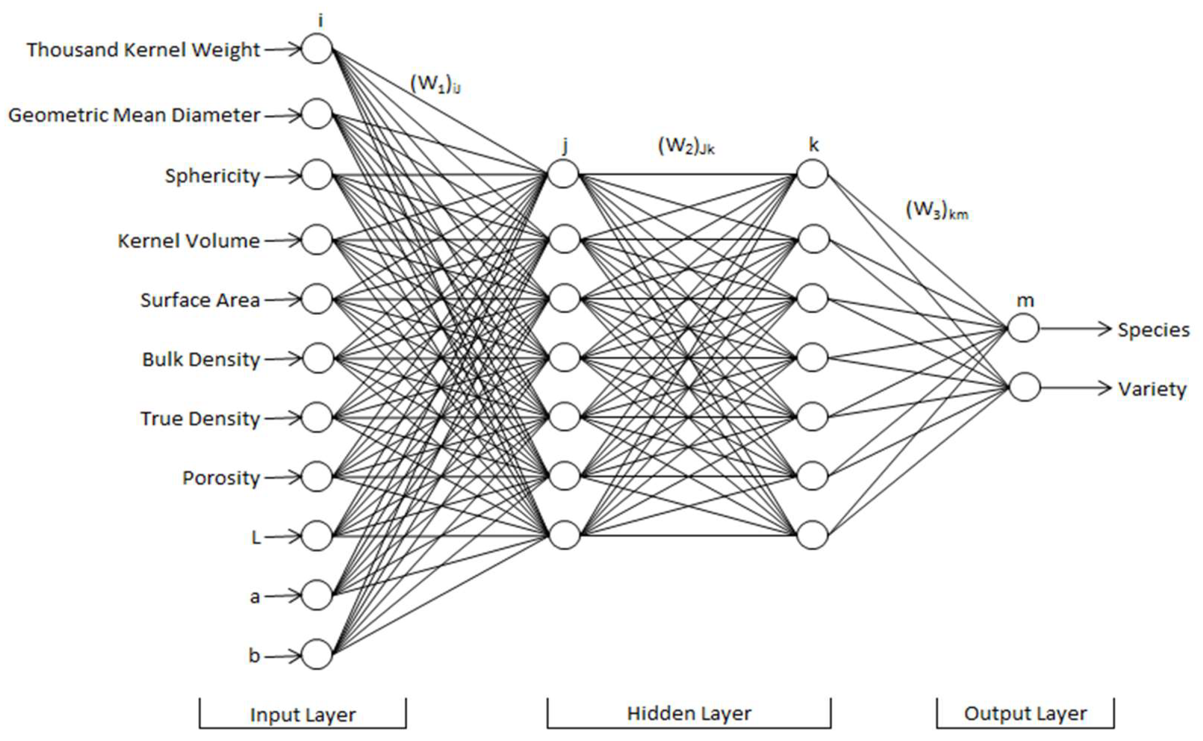
2.2. Artificial Neural Networks

The ANN model was developed by using the Matlab NN Toolbox (The Mathworks Inc., Natick, MA, USA). In the model, 539 data in total were used. In the ANN model, thousand kernel weight, geometric mean diameter, sphericity, kernel volume, surface area, bulk density, true density, porosity and colour parameters (L, a, b) were used as input parameters; and species and varieties as output parameters.

While establishing the ANN model, all the data were normalized between 0 and 1 [34].

For normalization, the following equation was used:

$$y_{nor}=\frac{y-y_{min}}{y_{max}-y_{min}}$$

(7)

To obtain real values from the normalized values, “y” value was calculated using the same formula.

To develop the ANN model, normalized data were divided into two data sets of training and test. In the training set, 502 data were used, whereas 37 data in the test set. The numbers of the most fit neurons in the hidden layers were found to be in the range of 2–25 by the trial and error method. In the ANN model, to obtain the most fit epoch number, epoch numbers from 1 to 10,000 were tried. As a result of trials, the most fit epoch number for the model was determined.

In the ANN model, Feed Forward Back Propagation, Multilayer Perceptron network structure was used. The back-propagation algorithm in this network is the most popular and commonly used algorithm. It minimizes the total error by varying the weights in order to enhance the network performance [35,36]. The training algorithm used is the Levenberg-Marquart algorithm [37,38].

Training of the network was continued until the test error reaches the determined tolerance value. After training of the network ended successfully, the network was tested by test data [9].

In order to determine the performances of the results, RMSE and R² values that are considered to be principal accuracy measures and that are based on the concept of mean error and commonly used were calculated using the following formulas [39].

$$RMSE=\sqrt{\frac{{{\displaystyle \sum }}_1^m{(x_1-x)}^2}{m}}$$

(8)

$$R^2=1-\left[\sqrt{\frac{{{\displaystyle \sum }}_1^m{(x_1-x)}^2}{{{\displaystyle \sum }}_1^m{(x_1)}^2}}\right]$$

(9)

Here RMSE, Root Mean Square Error, R², coefficient of determination, m, number of data, x, real value and x₁, estimated value.

The error between real values and estimated ones was calculated by means of the following equation [40].

$$\mathsf{\epsilon }=\frac{100}{m}{\displaystyle \sum }_1^m\left|\frac{x-x_1}{x}\right|$$

(10)

Here ε, relative error, m, data number, x, real value and x₁, estimated value.

Data concerning the physical parameters obtained were evaluated by conducting a factorial experiment in a randomized complete block design, using the JMP statistical program (SAS Institute Inc., Cary, NC, USA) [41].

3. Results and Discussion

3.1. Physical Properties

The mean and standard deviation values of the physical properties of the varieties of species of bread wheat, durum wheat, barley, oat and triticale used in the study are given in

Table 2. The mean and standard deviation values of the physical properties of the grain varieties.

Species	Thousand Kernel Weight (g)	Geometric Mean Diameter (mm)	Sphericity (%)	Kernel Volume (mm3)	Surface Area (mm2)	Bulk Density (kg/m3)	True Density (kg/m3)	Porosity (%)	L	a	b
Bread Wheat	42.23 ± 0.036 c	3.93 ± 0.004 d	60.85 ± 0.062 a	21.04 ± 0.081 c	40.96 ± 0.119 d	773.17 ± 0.40 a	1271.88 ± 1.78 a	39.18 ± 0.096 d	49.11 ± 0.026 c	8.33 ± 0.01 b	17.84 ± 0.013 c
Durum Wheat	48.47 ± 0.057 a	4.16 ± 0.007 c	54.05 ± 0.098 b	23.73 ± 0.129 b	46.29 ± 0.190 c	745.56 ± 0.64 b	1270.65 ± 2.83 a	41.30 ± 0.153 c	48.66 ± 0.041 d	0.86 ± 0.016 a	17.65 ± 0.021 d
Barley	48.49 ± 0.067 a	4.44 ± 0.008 a	50.78 ± 0.116 d	28.11 ± 0.151 a	53.19 ± 0.223 b	679.43 ± 0.76 d	1202.84 ± 3.33 c	43.48 ± 0.179 b	58.43 ± 0.049 a	4.48 ± 0.019 e	18.71 ± 0.025 b
Oat	33.83 ± 0.078 d	4.30 ± 0.010 b	34.76 ± 0.134e	23.45 ± 0.175 b	55.22 ± 0.258 a	482.80 ± 0.87 e	997.36 ± 3.84 d	51.54 ± 0.207 a	55.36 ± 0.056 b	6.82 ± 0.022 d	19.00 ± 0.028 a
Triticale	44.60 ± 0.095 b	4.15 ± 0.012 c	52.71 ± 0.164 c	23.28 ± 0.214 b	46.22 ± 0.316 c	717.44 ± 1.07 c	1228.01 ± 4.70 b	41.58 ± 0.254 c	45.59 ± 0.069 e	7.29 ± 0.027 c	15.06 ± 0.035 e
Mean	43.59	4.10	54.81	22.96	45.57	720.21	1229.98	41.66	50.74	7.61	17.85
CV (%)	1.42	2.43	1.74	7.31	5.02	0.68	2.17	3.16	0.71	1.72	1.07
LSD(0.05)	0.25	0.03	0.42	0.56	0.82	2.81	12.33	0.66	0.18	0.07	0.09

Mean: Arithmetic mean. CV: Coefficient of Variation. LSD: Least Significant Difference.

. All of the physical properties are found to be statistically significant (p < 0.05).

3.2. Thousand Kernel Weight

The highest thousand kernel weight values were 48.47 g for durum wheat and 48.49 for barley, the lowest was 33.83 g for oat being placed at the last group. The highest thousand kernel weight was obtained by 56.80 g for durum wheat variety of Meram-2002. The lowest value obtained was 28.18 g for the oat variety of Faikbey. Babi´c et al. [42], in their study on bread wheat, obtained a mean thousand kernel weight of 44.01 g. Topal et al. [43], in their study on 16 lines and varieties of durum wheat, obtained a mean thousand kernel weight of 41.73 g. Güner [44] reported the mean thousand kernel weight to be 47.38 g for durum wheat. Dursun and Güner [45], in their study on barley, obtained a thousand kernel weight of 43 g; and Güner [44] obtained 38.18 g in another study. Molenda and Horabik [46], in their study on oat, found a mean thousand kernel weight of 35.6 g; and Nelson [47] found it to be 34.8 g.

3.3. Geometric Mean Diameter

Geometric mean diameter values varied from 3.93 mm to 4.44 mm. The highest value was obtained in barley, the lowest value was obtained in bread wheat. While the barley variety of Larende (4.60 mm) had the highest geometric mean diameter, the bread variety of Yakar-99 (3.71 mm) had the lowest value. Babi´c et al. [42], in their study on bread wheat, obtained the geometric mean diameter to be 3.13 mm; Markowski et al. [48] obtained it to be 4.13 mm. Güner [44] obtained the geometric mean diameter as 4.35 mm for durum wheat. In studies on barley, geometric mean diameters were reported to be 4.43 mm by Tavakoli et al. [49]; 4.38 mm by Güner [44] and 4.54 mm by Song and Litchfield [50].

3.4. Sphericity

Sphericity values ranged from 34.76% to 60.85%. The highest value was obtained in the bread wheat variety of Kınacı-97 (65.46%), the lowest value in the oat variety of Faikbey (32.44%). Markowski et al. [48], in their study on bread wheat, determined the sphericity value to be 57.12%. Güner [44] obtained the sphericity value of durum wheat to be 55.06%; and Topal et al. [43] obtained it as 50.56%. Tavakoli et al. [49], in their study on barley, found it to be 47.70% and Güner [44] found it as 46.10%.

3.5. Kernel Volume

Kernel volume values ranged from 21.04 mm³ to 28.11 mm³. The highest value was obtained in the barley variety of Larende (31.13 mm³), the lowest was obtained in the bread wheat variety of Karahan-99 (17.01 mm³). Markowski et al. [48], in their study on bread wheat, determined the kernel volume value to be 36.95 mm³. Güner [44], in his study, obtained the kernel volume of the durum wheat to be 35.76 mm³; Nelson [47] found it as 26.1 mm³. Güner [44], in his studies on barley, obtained the kernel volume to be 38.37 mm³. Nelson [47] obtained the mean kernel volume to be 21.4 mm³ for spring oat and 26.8 mm³ for winter oat.

3.6. Surface Area

Whereas oat (55.22 mm²) had the largest surface area, bread wheat (40.96 mm²) had the lowest value. Babi´c et al. [42], in their study on bread wheat, obtained the surface area to be 30.07 mm². Topal et al. [43], in their study, reported that they found the surface area of durum wheat to be 26.93 mm². Güner [44], in his study, obtained the surface area of barley to be 25.10 mm².

3.7. Bulk Density

Bulk density values varied from 482.80 kg/m³ to 773.17 kg/m³. The highest value obtained was in the wheat variety of Pehlivan (804.44 kg/m³), the lowest value in the oat variety of Argentina (449.99 kg/m³). Markowski et al. [48], in their study on bread wheat, reported the bulk density value to be 732.57 kg/m³. In studies on durum wheat, bulk density values were reported by Nelson [47] 788 kg/m³, Güner [44] 815 kg/m³ and Sokhansanj and Lang [51] 760 kg/m³. In the studies on oat by different researchers, bulk density values varied in the range of 412–576 kg/m³ [23,46,47].

3.8. True Density

True density values ranged from 997.36 kg/m³ to 1271.88 kg/m³. The highest value obtained in the bread wheat of Alpu 2001 (1316.20 kg/m³), the lowest value in the oat variety of Argentina (954.32 kg/m³). Markowski et al. [48], in their study on bread wheat, reported the true density as 1382.17 kg/m³. Nelson [47] obtained the true density value for durum wheat to be 1411 kg/m³. In other durum wheat studies, the true density value was obtained by Güner [44] 1325 kg/m³; Sokhansanj and Lang [51] 1370 kg/m³. Güner [44], in his study on barley, obtained the true density as 995 kg/m³. Nelson [47] found a mean true density value of 1314 kg/m³ for spring oat and 1295 kg/m³ for winter oat. In other studies on oat, true density values varied in the range of 950–1397 kg/m³ [23,46].

3.9. Porosity

Porosity values varied from 39.18% to 51.54%. The highest value obtained in the oat line of Y-1779 (53.42%), the lowest value in the bread wheat variety of Kınacı-97 (37.48%). Markowski et al. [48], in their study on bread wheat, reported the porosity value to be 46.9%. Whereas Güner [44] found the porosity value to be 38.49%, Sokhansanj and Lang [51] found it to be 45%. Güner [44] obtained the porosity value 31.25% for barley. Molenda and Horabik [46], in their study, obtained the porosity values of in the range of 59.5–62.5% for oat.

3.10. Colour

Values of colour parameters (L, a, b) belonging to varieties are given in Table 2. On average, L, a and b values were obtained to be 50.74, 7.61 and 17.85, respectively. It was determined that there had been a statistically significant difference between species and varieties (p < 0.05). Colour differences in the classification of varieties in wheat are important [4].

All the physical parameters evaluated are placed at statistically different groups indicated that each of these parameters is important in classification of varieties.

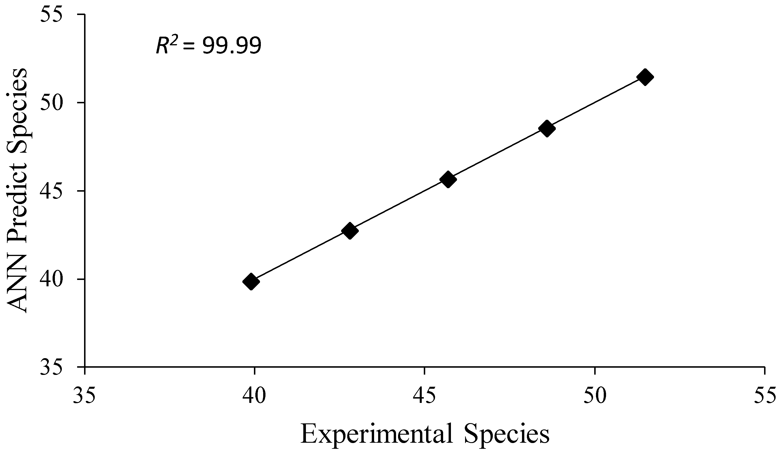
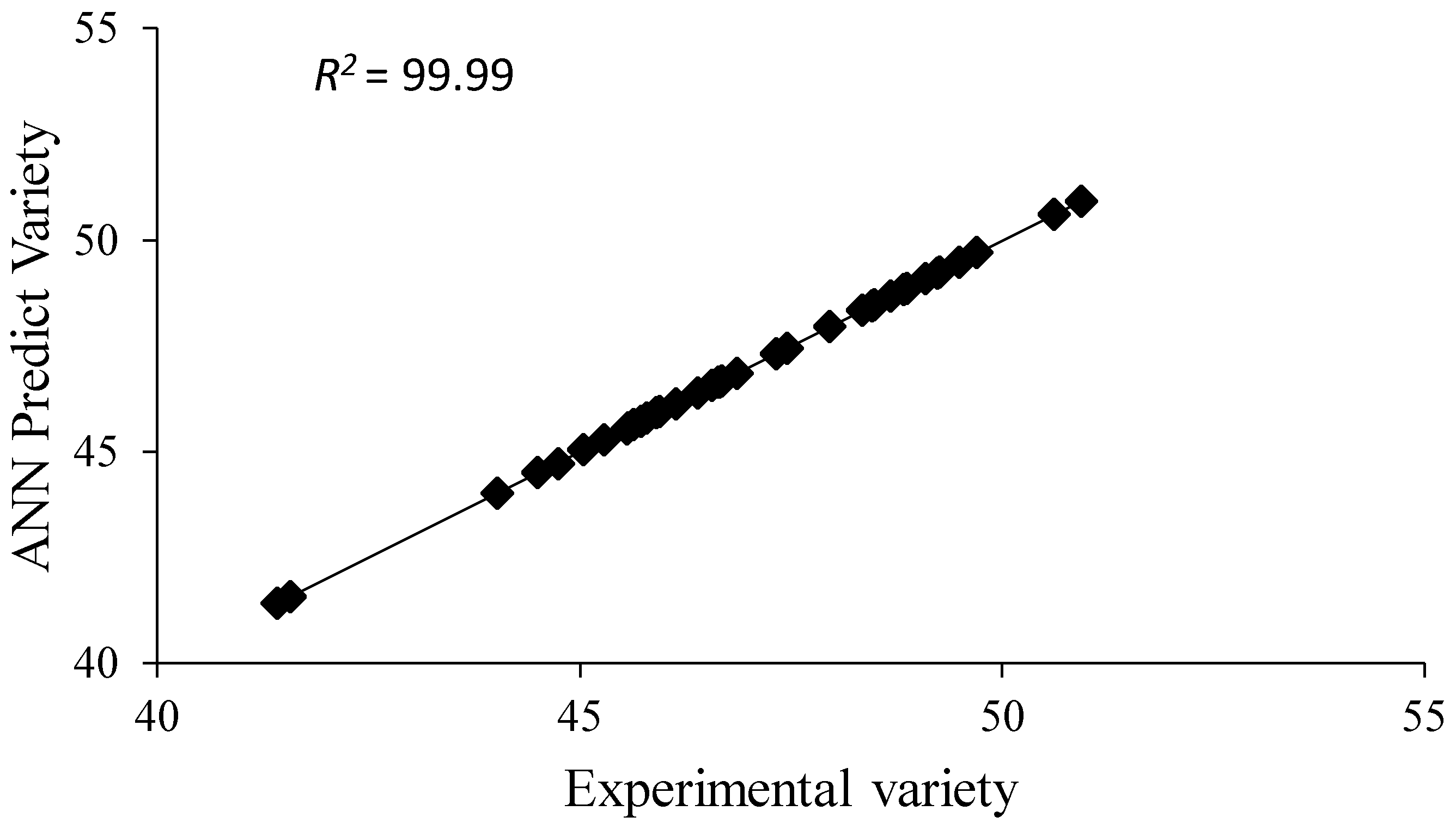
3.11. Artificial Neural Networks

In the ANN model, the structure of the network was designed in the form of 11-(7-7)-2, consisting of 11 input, 2 hidden and 2 output layers (Figure 1). As training algorithm, the Levenberg-Marquart algorithm was used [37,38], As transfer function, tansig was used in the first hidden layer, logsig in the second hidden layer; and linear functions were used in the output layer. For the network, the lowest training error was obtained at the epoch number of 10,000.

The mathematical formula of the ANN model is given in the following equation.

$$y_m={\displaystyle \sum }_1^k{(W_3)}_{k,m}{F}_k+b_k$$

(11)

LOGSIG transfer function for the second hidden layer (F_k),

$$F_k=\frac{1}{(1+e^{(-NE{T}_k)})}$$

(12)

$$NE{T}_k={\displaystyle \sum }_1^j{(W_2)}_{j,k}{F}_j+b_j$$

(13)

TANSIG transfer function for the first hidden layer (F_j),

$$F_j=\frac{2}{(1+e^{(-2NE{T}_j)})}-1$$

(14)

$$NE{T}_j={\displaystyle \sum }_1^i{(W_1)}_{i,j}{x}_1+b_i$$

(15)

were calculated using the equations above. In these equations; i, number of inputs, j, number of neurons in the first hidden layer, k, number of neurons in the second hidden layer, m, number of outputs, W₁, W₂, W₃, connection weight, x, input parameter, y_m, output parameter and b, bias. Weights are given in

Table 3. Connection weight values for Equation (15).

(J)	(W1)i1	(W1)i2	(W1)i3	(W1)i4	(W1)i5	(W1)i6	(W1)i7	(W1)i8	(W1)i9	(W1)i10	(W1)i11
1	0.5722	−0.1842	0.2088	−0.4904	0.8882	0.0004	0.1553	−0.2154	0.0294	0.2401	0.0727
2	0.1007	0.7627	−0.2897	0.4454	−1.485	−1.0178	0.7479	−0.7256	−0.3673	0.0447	−0.4264
3	−0.0103	0.0607	−0.0985	0.0191	−0.0794	−0.0455	−0.0053	−0.0056	−0.0095	−0.0704	−0.0183
4	−3.8002	7.4396	2.5305	−15.66	10.0015	−39.2805	26.9969	−27.0111	2.3286	−4.7543	−3.5571
5	3.1613	10.7492	−8.5456	7.0885	−22.8294	7.962	−8.0335	7.4794	0.9506	0.1078	−1.782
6	−0.0105	0.0993	−0.1542	0.0196	−0.1033	−0.0662	−0.0115	−0.0028	−0.0117	−0.1014	−0.0257
7	−0.0855	−0.7741	0.1382	−0.4588	1.6941	−0.0753	−0.0859	0.1043	0.1076	1.8165	0.1336

,

Table 4. Connection weight values for Equation (13).

(k)	(W2)j1	(W2)j2	(W2)j3	(W2)j4	(W2)j5	(W2)j6	(W2)j7
1	−5.1431	70.406	−4.5058	−18.016	−11.9865	−7.7543	15.8411
2	−0.1415	0.0677	−40.336	−0.0007	−0.0007	19.4536	−0.0737
3	51.1274	85.4875	−25.997	66.2967	50.4012	−36.0585	−67.172
4	−32.12	−63.85	−4.2685	15.3922	5.191	1.8093	29.4206
5	0.3936	−0.2782	18.4034	0.1364	0.1275	−13.0859	−4.0637
6	6.5031	−57.464	−8.112	−13.945	78.3948	−9.5059	81.1453
7	−14.722	−56.893	17.9144	−18.052	−13.727	13.933	8.3927

and

Table 5. Connection weight values for Equation (11).

(m)	(W3)k1	(W3)k2	(W3)k3	(W3)k4	(W3)k5	(W3)k6	(W3)k7
1	−0.007	32.1518	−0.0078	−0.0003	10.3896	0.0001	−0.0089
2	0.25	−0.0002	0.75	1	0.0006	0.25	0

and bias values in

Table 6. Bias values.

Number of Neurons	bi	bj	bk
1	−1.2269	2.1839	−15.7802
2	1.4557	13.8917	−0.2506
3	0.8503	−63.862
4	23.8469	−23.8218
5	2.7217	2.2416
6	0.7096	−32.6007
7	−1.2706	30.4023

.

Among the models obtained, the ANN model with the lowest RMSE and the highest R² value were determined to be the best fit. Whereas R² and RMSE values for species in the training set were found to be 0.99 and 0.000027, respectively; in the test set, they were found to be 0.99 and 0.000184, respectively. While R² and RMSE values for varieties in the training set were found to be 0.99 and 0.000318, respectively; in the test set, they were found to be 0.99 and 0.000624 (

Table 7. Performance of the ANN model.

Output	Training Set		Test Set
	RMSE	R2	RMSE	R2
Species	0.000027	0.99	0.000184	0.99
Variety	0.000318	0.99	0.000624	0.99

).

Coefficient of determination (R²) of the correlation between experimental data and the predicted values from the ANN model was found to be 99.99% for both species and varieties (Figure 2 and Figure 3).

Experimental data, predicted values calculated from the ANN model and the error values between them are given in

Table 8. Test and error values for the ANN model.

Variety	Variety			Species
	Experimental Data	Test Data	Error (%)	Experimental Data	Test Data	Error (%)
Sultan 95	49.26	49.26	0.004	39.89	39.89	0.000
Süzen 97	46.65	46.65	0.004	39.89	39.89	0.000
Tosunbey	47.96	47.96	0.001	39.89	39.89	0.000
Gerek 79	45.79	45.79	0.001	39.89	39.89	0.000
Alpu 2001	49.70	49.70	0.003	39.89	39.89	0.000
İkizce 96	45.05	45.06	0.016	39.89	39.89	0.000
Göksu-99	45.57	45.57	0.002	39.89	39.89	0.000
Konya-2002	46.57	46.57	0.004	39.89	39.89	0.000
Müfitbey	45.73	45.72	0.006	39.89	39.89	0.000
Kınacı-97	48.83	48.83	0.016	39.89	39.89	0.000
Bağcı-2002	46.68	46.68	0.001	39.89	39.89	0.000
Bayraktar 2000	45.91	45.92	0.008	39.89	39.89	0.000
Ahmetağa	45.64	45.64	0.006	39.89	39.89	0.000
Ekiz	47.45	47.45	0.001	39.89	39.89	0.000
Pehlivan	49.49	49.49	0.002	39.89	39.90	0.031
Altıntaç-95	46.64	46.64	0.001	42.78	42.78	0.008
Çeşit-1252	50.93	50.93	0.001	42.78	42.78	0.000
Mirzabey-2000	48.67	48.67	0.004	42.78	42.78	0.000
Meram-2002	50.61	50.61	0.003	42.78	42.78	0.000
Yılmaz-98	48.87	48.87	0.009	42.78	42.78	0.000
Kızıltan-91	48.34	48.34	0.008	42.78	42.78	0.000
Karatay 94	45.28	45.29	0.009	45.67	45.67	0.000
Çetin 2000	47.32	47.31	0.024	45.67	45.67	0.000
Larende	48.49	48.49	0.005	45.67	45.67	0.000
Avcı-2002	48.46	48.45	0.009	45.67	45.67	0.000
Kıral-97	44.75	44.72	0.069	45.67	45.67	0.000
Beyşehir	49.23	49.23	0.006	45.67	45.67	0.000
Aydanhanım	49.09	49.08	0.005	45.67	45.67	0.000
Karma 2000	46.40	46.39	0.005	48.57	48.57	0.000
Melez-2001	45.94	45.95	0.012	48.57	48.57	0.000
Mikham-2002	46.14	46.13	0.007	48.57	48.57	0.000
Samur Sortu	44.02	44.02	0.002	48.57	48.57	0.002
Y-1779	45.55	45.54	0.034	51.46	51.46	0.000
Checota	44.50	44.50	0.010	51.46	51.46	0.000
Argentina	41.43	41.43	0.002	51.46	51.46	0.000
Seydişehir	46.86	46.85	0.035	51.46	51.46	0.000
Faikbey	41.58	41.57	0.011	51.46	51.46	0.000
Mean Error	0.009					0.001

. The mean error value for variety was found to be 0.009% and 0.001% for species.

4. Conclusions

The physical parameters of agricultural materials are important to have an accurate estimate of physical features and other characteristics which can be considered as engineering parameters for that product. These parameters such as the length, width, thickness, arithmetic mean diameter, geometric mean diameter, sphericity, volume, thousand seed mass, bulk density, true density, porosity and surface area are used in the grading, handling, sieving, storage, drying, processing and designing equipment.

11 physical properties for species grown in Turkey were determined. It was determined that these properties found to be statistically different could be used to classify species and varieties.

In the study, an Artificial Neural Network model was developed for classification. The structure of the model was set up to consist of 11 input, 2 hidden and 2 output layers. Using tansig and logsig transfer functions in the hidden layers and linear function in the output layer, the lowest error value was obtained.

In the developed model, R² values for the species and varieties were found to be 0.99 for both; and RMSE values to be 0.000184 and 0.000624, respectively. The mean errors in approximation to the experimental data were obtained to be 0.001% and 0.009% for species and varieties, respectively. It has shown that all the results acquired from the developed ANN model had a good alignment with the experimental data.

Explaining two subjects (species and variety) by a single model obtained with ANN shows that the ANN offers a significant ease of use. It will enable to manufacture more easily, simply and economically the equipment to be developed thanks to this model.

It would be possible to construct automation systems, using the ANN model developed, for classifying and cleaning grains to use in Commodity Exchanges and milling factories.

References

1. Neuman, M.; Sapirstein, H.D.; Shwedyk, E.; Bushuk, W. Discrimination of wheat class and variety by digital image analysis of whole grain samples. J. Cereal Sci. 1987, 6, 125–132. [Google Scholar] [CrossRef]
2. Barker, D.A.; Vouri, T.A.; Hegedus, M.R.; Myers, D.G. The use of ray parameters for the discrimination of Australian wheat varieties. Plant Var. Seeds 1992, 5, 35–45. [Google Scholar]
3. Chen, X.; Xun, Y.; Li, W.; Zhang, J. Combining discriminant analysis and neural networks for corn variety identification. Comput. Electron. Agric. 2010, 71, 48–53. [Google Scholar] [CrossRef]
4. Pourreza, A.; Pourreza, H.R.; Abbaspour-Fard, M.H.; Sadrnia, H. Identification of nine Iranian wheat seed varieties by textural analysis with image processing. Comput. Electron. Agric. 2012, 83, 102–108. [Google Scholar] [CrossRef]
5. Mohsenin, N.N. Physical Properties of Plant and Animal Materials; Gordon and Breach Science Publishers Inc.: New York, NY, USA, 1970. [Google Scholar]
6. Tabatabaeefar, A. Moisture-dependent physical properties of wheat. Int. Agrophys. 2003, 17, 207–211. [Google Scholar]
7. Kalogirou, S.A. Applications of artificial neural networks in energy systems. Comput. Electron. Agric. 1999, 40, 1073–1087. [Google Scholar] [CrossRef]
8. Aydogan, H.; Altun, A.A.; Ozcelik, A.E. Performance analysis of a turbo charged diesel engine using biodiesel with back propagation artificial neural network. Energy Educ. Sci. Technol-A. 2011, 28, 459–468. [Google Scholar]
9. Visen, N.S.; Paliwal, J.; Jayas, D.S.; White, N.D.G. Specialist neural networks for cereal grain classification. Biosyst. Eng. 2002, 82, 151–159. [Google Scholar] [CrossRef]
10. Dubey, B.P.; Bhagwat, S.G.; Shouche, S.P.; Sainis, J.K. Potential of artificial neural networks in varietal identification using morphometry of wheat grains. Biosyst. Eng. 2006, 95, 61–67. [Google Scholar] [CrossRef]
11. Kalogirou, S.A. Artificial neural networks in the renewable energy systems applications: A review. Renew. Sustain. Energy Rev. 2001, 5, 373–401. [Google Scholar] [CrossRef]
12. Paliwal, J.; Visen, N.S.; Jayas, D.S. Evaluation of neural network architectures for cereal grain classification using morphological features. J. Agric. Eng. Res. 2001, 79, 361–370. [Google Scholar] [CrossRef]
13. Wang, N.; Dowell, F.; Zhang, N. Determining wheat vitreousness using image processing and a neural network. Presented at the 2002 ASAE Annual International Meeting/CIGR XVth World Congress, Chicago, IL, USA, 28–31 July 2002. [Google Scholar]
14. Visen, N.S.; Jayas, D.S.; Paliwal, J.; White, N.D.G. Comparison of two neural network architectures for classification of singulated cereal grains. Can. Biosyst. Eng. 2004, 46, 7–14. [Google Scholar]
15. Baykan, Ö.K.; Babalık, A.; Botsalı, F.M. Recognition of wheat type using artificial neural network. Presented at the 4th International Advanced Technologies Symposium, Konya, Turkey, 28–30 September 2005. [Google Scholar]
16. Babalık, A.; Baykan, Ö.K.; Botsalı, F.M. Determination of wheat kernel type by using image processing techniques and ANN. Presented at the International Conference on Modelling and Simulating, Konya, Turkey, 28–30 August 2006. [Google Scholar]
17. Pazoki, A.R.; Pazoki, Z. Classification system for rain fed wheat grain cultivars using artificial neural network. Afr. J. Biotechnol. 2011, 10, 8031–8038. [Google Scholar]
18. Taner, A.; Tekgüler, A.; Sauk, H.; Demirel, B. Classification of oat varieties by using artificial neural networks. Presented at the 27th National Congress of Agricultural Mechanization, Samsun, Turkey, 5–7 September 2012. [Google Scholar]
19. Liao, K.; Paulsen, M.R.; Reid, J.F.; Ni, B.C.; Bonifacio-Maghirang, E.P. Corn kernel breakage classification by machine vision using a neural network classifier. Trans. ASAE 1993, 36, 1949–1953. [Google Scholar] [CrossRef]
20. Romaniuk, M.D.; Sokhansanj, S.; Wood, H.C. Barley seed recognition using a multi-layer neural network. Presented at the 1993 International ASAE Winter Meeting, Chicago, IL, USA, 14–17 December 1993. [Google Scholar]
21. Jayas, D.S.; Paliwal, J.; Visen, N.S. Multi-layer neural networks for image analysis of agricultural products. J. Agric. Eng. Res. 2000, 77, 119–128. [Google Scholar] [CrossRef]
22. Federico, M.; Remo, B.; Antonio, L.M.; Andrea, D.M.; Rita, A.; Roberta, F. Classification of 6 durum wheat cultivars from Sicily (Italy) using artificial neural networks. Chemometr. Intell. Lab. Syst. 2008, 90, 1–7. [Google Scholar]
23. Wang, Z.; Cong, P.; Zhou, J.; Zhu, Z. Method for identification of external quality of wheat grain based on image processing and artificial neural network. Trans. CSAE 2007, 23, 158–161. [Google Scholar]
24. Zapotoczny, P. Discrimination of wheat grain varieties using image analysis and neural networks. Part I. Single kernel texture. J. Cereal Sci. 2011, 54, 60–68. [Google Scholar]
25. Jain, R.K.; Bal, S. Properties of pearl millet. J. Agric. Eng. Res. 1997, 66, 85–91. [Google Scholar] [CrossRef]
26. Hacıseferogulları, H.; Özcan, M.; Demir, F.; Çalışır, S. Some nutritional and technological properties of garlic (Allium sativum L.). J. Food Eng. 2005, 68, 463–469. [Google Scholar] [CrossRef]
27. Bell, M.; Fischer, R.A. Guide to Plant and Crop Sampling: Measurement and Observations for Agronomic and Physiological Research in Small Grain Cereals; Wheat Special Report No. 32; CIMMYT: Veracruz, Mexico, 1994. [Google Scholar]
28. Cölkesen, M.; Öktem, A.; Eren, N.; Akıncı, C. Determination of suitable durum wheat varieties on dry and irrigated conditions in şanliurfa. Presented at the Symposium of Durum Wheat and Products, Ankara, Turkey, 30 November–3 December 1993. [Google Scholar]
29. Aviara, N.A.; Gwandzang, M.I.; Haque, M.A. Physical properties of guna seeds. J. Agric. Eng. Res. 1999, 73, 105–111. [Google Scholar] [CrossRef]
30. Sacilik, K.; Oztürk, R.; Keskin, R. Some physical properties of hemp seed. Biosyst. Eng. 2003, 86, 191–198. [Google Scholar] [CrossRef]
31. Ogunjimi, L.O.; Aviara, N.A.; Aregbesola, O.A. Some engineering properties of locust bean seed. J. Food Eng. 2002, 55, 95–99. [Google Scholar] [CrossRef]
32. Smedley, S.M. Discrimination between beers with small colour differences using the CIELAB colour space. J. Inst. Brew. 1995, 101, 195–201. [Google Scholar] [CrossRef]
33. Connolly, C.; Fleiss, T. A study of efficiency and accuracy in the transformation from RGB to CIELAB colour space. IEEE Trans. Image Process. 1997, 6, 1046–1048. [Google Scholar] [CrossRef] [PubMed]
34. Purushothaman, S.; Srinivasa, Y.G. A back-propagation algorithm applied to tool wear monitoring. Int. J. Mach. Tool Manuf. 1994, 34, 625–631. [Google Scholar] [CrossRef]
35. Jacobs, R.A. Increased rate of convergence through learning rate adaptation. Neural Netw. 1988, 1, 295–307. [Google Scholar] [CrossRef]
36. Minai, A.A.; Williams, R.D. Back-propagation heuristics: A study of the extended delta-bar-delta algorithm. In Proceedings of the 1990 IJCNN International Joint Conference on Neural Networks, San Diego, CA, USA, 17–21 June 1990. [Google Scholar]
37. Levenberg, K. A method for the solution of certain nonlinear problems in least squares. Quart. Appl. Math. 1944, 2, 164–168. [Google Scholar] [CrossRef]
38. Marquart, D.W. An algorithm for least-squares estimation of nonlinear parameters. J. Soc. Ind. Appl. Math. 1963, 11, 431–441. [Google Scholar] [CrossRef]
39. Bechtler, H.; Browne, M.W.; Bansal, P.K.; Kecman, V. New approach to dynamic modelling of vapour-compression liquid chillers: Artificial neural networks. Appl. Therm. Eng. 2001, 21, 941–953. [Google Scholar] [CrossRef]
40. Taner, A.; Tekgüler, A.; Sauk, H. Classification of durum wheat varieties by artificial neural networks. Anadolu J. Agric. Sci. 2015, 30, 51–59. [Google Scholar] [CrossRef]
41. Yurtsever, N. Experimental Statistical Methods; Soil and Fertilizer Research Institute, The Global Forum on Agricultural Research and Innovation: Ankara, Turkey, 1984. [Google Scholar]
42. Babi´c, L.; Babi´c, M.; Turan, J.; Mati´c-Keki´c, S.; Radojˇcin, M.; Mehandˇzi´c-Staniˇsi´c, S.; Pavkov, I.; Zoranovi´c, M. Physical and stress-strain properties of wheat (Triticum aestivum) kernel. J. Sci. Food Agric. 2011, 91, 1236–1243. [Google Scholar] [CrossRef] [PubMed]
43. Topal, A.; Aydın, C.; Akgün, N.; Babaoglu, M. Diallel cross analysis in durum wheat (Triticum durum Desf.): Identification of best parents for some kernel physical features. Field Crop Res. 2004, 87, 1–12. [Google Scholar] [CrossRef]
44. Güner, M. Pneumatic conveying characteristics of some agricultural seeds. J. Food Eng. 2007, 80, 904–913. [Google Scholar] [CrossRef]
45. Dursun, E.; Güner, M. Determination of mechanical behaviour of wheat and barley under compression loading. J. Agric. Sci. 2003, 9, 415–420. [Google Scholar]
46. Molenda, M.; Horabik, J. Part1: Characterization of mechanical properties of particulate solids for storage and handling. In Mechanical Properties of Granular Agro-Materials and Food Powders for Industrial Practice; Molenda, M., Horabik, J., Eds.; Institute of Agrophysics Polish Academy of Sciences: Lublin, Poland, 2005. [Google Scholar]
47. Nelson, S.O. Dimensional and density data for seeds of cereal grain and other crops. Trans. ASAE 2002, 45, 165–170. [Google Scholar] [CrossRef]
48. Markowski, M.; Zuk-Golaszewska, K.; Kwiatkowski, D. Influence of variety on selected physical and mechanical properties of wheat. Ind. Crop Prod. 2013, 47, 113–117. [Google Scholar] [CrossRef]
49. Tavakoli, M.; Tavakoli, H.; Rajabipour, A.; Ahmadi, H.; Gharib-Zahedi, S.M.T. Moisture-dependent physical properties of barley grains. Int. J. Agric. Biol. Eng. 2009, 2, 84–91. [Google Scholar] [CrossRef]
50. Song, H.; Litchfield, J.B. Predicting method of terminal velocity for grains. Trans. ASAE 1991, 34, 225–231. [Google Scholar] [CrossRef]
51. Sokhansanj, S.; Lang, W. Prediction of kernel and bulk volüme of wheat and canola during adsorption and desorption. J. Agric. Eng. Res. 1996, 63, 129–136. [Google Scholar] [CrossRef]
Figure 1. The Artificial Neural Network (ANN) structure.
Agronomy 08 00123 g001
Figure 2. Regression graphics between ANN-predicted values and experimental data for species.
Agronomy 08 00123 g002
Figure 3. Regression graphics between ANN-predicted values and experimental data for variety.
Agronomy 08 00123 g003