Role of Modelling in International Crop Research: Overview and Some Case Studies

 , , , , ,
Abstract
1. Introduction
2. Basic Principles and History of Crop Modelling
2.1. Environment
2.2. Management
2.3. Genotype
2.4. Socioeconomics
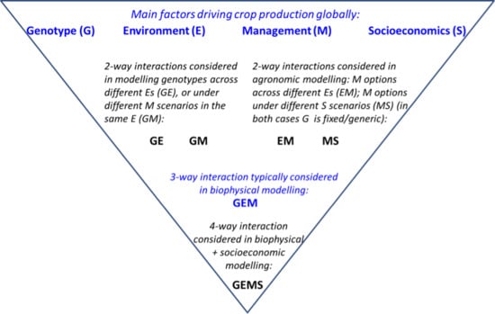
2.5. Interactions
3. Modelling the Environment
3.1. The Physical Environment
3.2. Tools for Monitoring and Managing Pests and Diseases
Case Study: Insect Life Cycle Modelling Software for Pest and Disease Management
4. Modelling Crop Management
4.1. Crop Models for Management Practices
Case Study: Exploring Sustainable Crop Management Options to Reduce Groundwater Table Decline in Northwest India
- If minimizing permanent loss of water from the system is the objective, the best method is a partial conservation agriculture rice-wheat system with a short duration rice variety.
- If maximizing productivity is the sole objective, a full conservation agriculture system with a medium duration variety is the best option.
- Replacing rice with rainy season maize (Zea mays L.) in the system can maintain yields while reducing the total irrigation amount by ~80%, which can contribute to huge reductions in pumping costs and energy use. Maize-based systems also reduce permanent water loss from the system by 200 mm (Figure 3).
4.2. E × M Interactions
Case Study: Irrigation Scheduling in Bangladesh’s Ganges Delta Region
4.3. M × S Interactions
4.4. Technological Innovations Aiding Crop Management Models
Case Study: Anomalies in Irrigation Experiments in Maize Farmer’s Fields Detected with Remote Sensors
5. Modelling Genetic Variability
5.1. Crop Simulation Models for Genetic Improvement
5.2. Genomic Selection Models Incorporating Physiological Traits and Insights
5.3. G × E Interactions
5.4. G × E × M Interactions
- Statistical modelling of G × E × M (and lower order interactions) as a stochastic tool for testing specific elements of simulation models and to parameterize or calibrate input variables;
- Genomic selection models using high density molecular markers to parameterize G and thus test the value of specific genomic regions and make predictions in different target environments [115];
- Physiological breeding models to test different combinations of traits and alleles through strategic crossing and progeny testing in well-defined target environments [7];
- Testing of G × M interactions, which lend well to reductionist research approaches because—unlike E, which is infinitely variable in the field—M can be varied for one or more factor within a single E.
6. Modelling Socioeconomic Factors
6.1. Bio-Economic Modelling
6.2. Foresight Analysis
6.3. Case Study: Calculating Food Systems Risks
7. Increasing the Availability of Data and Its Value in Modelling
7.1. Global Phenotyping Networks
7.2. Data Sharing and Standardization
8. Conclusions
- New insights into the biology of plant development and response to environmental cues will naturally enable model development, as it becomes possible to incorporate additional functions into the main algorithms of models. While this will contribute to a continuous improvement, it contains an inherent risk of making models so complex that they lose their initial purpose of being a simpler representation of the reality, but not the reality itself. A recent paper by Soltani and Sinclair [309] illustrates the value of keeping models simple. While continuous improvements to the science of crop models are critical, there should be a balance between the level of complexity and approximation of the processes they model.
- While crop models are primarily being developed and used as scientific research tools, their stakeholders extend far beyond research institutions to include farmers, policymakers, development practitioners, and the private sector. Maintaining close links with this international community is a crucial part of developing and applying models, and one where CGIAR centres can play a major role through their network of public and private sector partners at all levels. Coordinated linkages between stakeholders will help define the crop modelling community’s priorities and stimulate further development in the modelling science, as well as transparently communicate the capacity and caveats of crop modelling approaches. For example, crop models are increasingly equipped to provide stochastic estimates of crop growth and yields (e.g., Yield Prophet®) and potential impacts of altering specific genetic or agronomic traits (e.g., [370]). Meanwhile, foresight studies increasingly incorporate crop models and couple them with large-scale economic models to address questions from policymakers on the potential impacts of global change scenarios.
- Scientists, including many working in CGIAR Centres, are progressively picking robust and complex methods from advanced mathematics, computer science, and physics principles to address the challenges outlined in this review. Artificial neural networks and cellular automata, coupled with fuzzy logic percolation and individual/agent-based approaches, are among the modelling methods being applied to improving crop management (Figure 2). Artificial neural networks are a system inspired by the functioning of neural networks of animal brains [371]. Its main advance is that it permits the use of data collected at any suitable scale, bypassing the ambiguities that can occur when fitting equations to estimated parameters [371]. Meanwhile cellular automate is a spatially and temporally discrete modelling concept that describes the dynamics through interactions and synchronous evolution using elements such as grid of cells, states, neighbourhood, transition rules, and time step [372]. This approach, when coupled with fuzzy logic (i.e., representation of the level of truth with scaled values from 0 and 1), yields a robust model capable of incorporating vague and imprecise knowledge to guide and improve pest management [372].
- As great strides are made in harnessing the genotypic information of more and more traits, the potential exists to interface a layer of genetic information within crop coefficients. Crop coefficient(s), leading to a specific response, could be driven by QTL with a value of putative effect. This kind of progress would theoretically enable the prediction of ideotype performance, based on marker content [373,374,375]. However, more knowledge is needed to better understand epistatic interactions and their role in determining phenotypes.
- Genomic selection is increasingly being used to select promising recombinants, based on their marker content. Genomic selection has shown that breeding can be done saving time and money and thus improving the genetic gains. Crop models could therefore be interfaced to deal with the portion of the phenotypic variance that is accounted for by these interactions.
- The G × E × M × S paradigm offers scope to address the complexities of agri-food systems, using data and models, without falling into the trap of over-simplification, inherent in modelling, by harnessing data and tools across multiple scientific disciplines and thus, enhancing the potential for creating impact for the target beneficiaries of the CGIAR.
Author Contributions
Funding
Acknowledgments
Conflicts of Interest
References
- Grassini, P.; Eskridge, K.M.; Cassman, K.G. Distinguishing between yield advances and yield plateaus in historical crop production trends. Nat. Commun. 2013, 4, 2918. [Google Scholar] [CrossRef] [PubMed]
- Wiebe, K.; Lotze-Campen, H.; Sands, R.; Tabeau, A.; Van Der Mensbrugghe, D.; Biewald, A.; Bodirsky, B.; Islam, S.; Kavallari, A.; Mason-D’croz, D.; et al. Climate change impacts on agriculture in 2050 under a range of plausible socioeconomic and emissions scenarios. Environ. Res. Lett. 2015, 10, 085010. [Google Scholar] [CrossRef]
- Rosegrant, M.W.; Tokgoz, S.; Bhandary, P. The new normal? A tighter global agricultural supply and demand relation and its implications for food security. Am. J. Agric. Econ. 2013, 95, 303–309. [Google Scholar] [CrossRef]
- Fischer, R.A.; And, D.B.; Edmeades, G.O. Crop Yields and Global Food Security: Will Yield Increase Continue to Feed the World? Australian Centre for International Agricultural Research: Canberra, Australia, 2014; ISBN 978-1-925133-06-6. [Google Scholar]
- Antle, J.M.; Basso, B.; Conant, R.T.; Godfray, H.C.J.; Jones, J.W.; Herrero, M.; Howitt, R.E.; Keating, B.A.; Munoz-Carpena, R.; Rosenzweig, C.; et al. Towards a new generation of agricultural system data, models and knowledge products: Design and improvement. Agric. Syst. 2017, 155, 255–268. [Google Scholar] [CrossRef]
- Hodson, D.; White, J. GIS and Crop Simulation Modelling Applications in Climate Change Research. Clim. Chang. Crop Prod. 2010, 1, 245–262. [Google Scholar] [CrossRef]
- Reynolds, M.; Langridge, P. Physiological breeding. Curr. Opin. Plant Biol. 2016, 31, 162–171. [Google Scholar] [CrossRef] [PubMed]
- CIAT; IFPRI. CGIAR Big Data Coordination Platform. Leveraging CGIAR Data: Bringing Big Data to Agriculture, and Agriculture to Big Data; Proposal to the CGIAR Fund Council; International Center for Tropical Agriculture (CIAT): Cali, Colombia; International Food Policy Research Institute: Washington, DC, USA, 2016. [Google Scholar]
- Bassu, S.; Brisson, N.; Durand, J.L.; Boote, K.; Lizaso, J.; Jones, J.W.; Rosenzweig, C.; Ruane, A.C.; Adam, M.; Baron, C.; et al. How do various maize crop models vary in their responses to climate change factors? Glob. Chang. Biol. 2014, 20, 2301–2320. [Google Scholar] [CrossRef]
- Rosenzweig, C.; Jones, J.W.; Hatfield, J.L.; Ruane, A.C.; Boote, K.J.; Thorburn, P.; Antle, J.M.; Nelson, G.C.; Porter, C.; Janssen, S.; et al. The Agricultural Model Intercomparison and Improvement Project (AgMIP): Protocols and pilot studies. Agric. For. Meteorol. 2013, 170, 166–182. [Google Scholar] [CrossRef]
- Ruane, A.C.; Hudson, N.I.; Asseng, S.; Camarrano, D.; Ewert, F.; Martre, P.; Boote, K.J.; Thorburn, P.J.; Aggarwal, P.K.; Angulo, C.; et al. Multi-wheat-model ensemble responses to interannual climate variability. Environ. Model. Softw. 2016, 81, 86–101. [Google Scholar] [CrossRef]
- White, J.W.; Hunt, L.A.; Boote, K.J.; Jones, J.W.; Koo, J.; Kim, S.; Porter, C.H.; Wilkens, P.W.; Hoogenboom, G. Integrated description of agricultural field experiments and production: The ICASA Version 2.0 data standards. Comput. Electron. Agric. 2013, 96, 1–12. [Google Scholar] [CrossRef]
- Reynolds, M.P.; Braun, H.J.; Cavalieri, A.J.; Chapotin, S.; Davies, W.J.; Ellul, P.; Feuillet, C.; Govaerts, B.; Kropff, M.J.; Lucas, H.; et al. Improving global integration of crop research. Science 2017, 357, 359–360. [Google Scholar] [CrossRef] [PubMed]
- Jones, J.W.; Antle, J.M.; Basso, B.; Boote, K.J.; Conant, R.T.; Foster, I.; Godfray, H.C.J.; Herrero, M.; Howitt, R.E.; Janssen, S.; et al. Brief history of agricultural systems modeling. Agric. Syst. 2017, 155, 240–254. [Google Scholar] [CrossRef] [PubMed]
- Whisler, F.D. Sensitivity Tests of the Crop Variables in Ricemod; IRRI Research Paper Series; International Rice Research Institute: Los Baños, Philippines, 1983; 14p. [Google Scholar]
- Kropff, M.J.; Cassman, K.G.; Van Laar, H.H.; Peng, S. Nitrogen and yield potential of irrigated rice. Plant Soil 1993, 155–156, 391–394. [Google Scholar] [CrossRef]
- Kropff, M.J.; van Laar, H.H.; CAB International; International Rice Research Institute. Modelling Crop-Weed Interactions; Kropff, M.J., van Laar, H.H., Eds.; CAB International: Wallingford, UK; International Rice Research Institute: Los Banos, Philipines, 1993; ISBN 9712200388. [Google Scholar]
- Kropff, M.J.; Van Laar, H.H.; Matthews, R.B. ORYZA1: An Ecophysiological Model for Irrigated Rice Production; DLO-Research Institute for Agrobiology and Soil Fertility: Wageningen, The Netherlands, 1994; ISBN 9073384230. [Google Scholar]
- Wopereis, M.C.S.; Bouman, B.A.M.; Kropff, M.J.; ten Berge, H.F.M.; Maligaya, A.R. Water use efficiency of flooded rice fields I. Validation of the soil-water balance model SAWAH. Agric. Water Manag. 1994, 26, 277–289. [Google Scholar] [CrossRef]
- Kropff, M.J.; Teng, P.S.; Rabbinge, R. The challenge of linking pest and crop models. Agric. Syst. 1995, 49, 413–434. [Google Scholar] [CrossRef]
- Matthews, R.B.; Kropff, M.J.; Bachelet, D.; Van Laar, H.H. (Eds.) Modeling the Impact of Climate Change on Rice Production in Asia; CAB International, in association with IRRI: Wallingford, UK, 1995; ISBN 0-85198-959-4. [Google Scholar]
- Aggarwal, P.K.; Kropff, M.J.; Cassman, K.G.; Berge, H.F.M. Simulating genotypic strategies for increasing rice yield potential in irrigated, tropical environments. Field Crops Res. 1997, 51, 5–17. [Google Scholar] [CrossRef]
- Kropff, M.J.; Teng, P.; Aggarwal, P.K.; Bouma, J.; Bouman, B.A.M.; Jones, J.W.; Van Laar, H.H. Applications of Systems Approaches at the Field Level. Volume 2: Proceedings of the Second International Symposium on Systems Approaches for Agricultural Development, held at IRRI, Los Baños, Philippines, 6–8 December 1995, 1st ed.; Springer: Cham, Switzerland, 1997; ISBN 978-0-7923-4286-1. [Google Scholar]
- Teng, P.S.; Kropff, M.J.; Ten-Berge, H.F.M.; Dent, J.B.; Lansigan, F.P.; Van-Laar, H.H. Applications of Systems Approaches at the Farm and Regional Levels. Volume 1: Proceedings of the Second International Symposium on Systems Approaches for Agricultural Development, held at IRRI, Los Banos, Philippines, 6–8 December 1995, 1st ed.; Springer: Cham, Switzerland, 1997; ISBN 9789401062787. [Google Scholar]
- Dingkuhn, M.; Sow, A.; Samb, A.; Diack, S.; Asch, F. Climatic determinants of irrigated rice performance in the Sahel—I. Photothermal and micro-climatic responses of flowering. Agric. Syst. 1995, 48, 385–410. [Google Scholar] [CrossRef]
- Dingkuhn, M.; Miezan, K.M. Climatic determinants of irrigated rice performance in the Sahel—II. Validation of photothermal constants and characterization of genotypes. Agric. Syst. 1995, 48, 411–433. [Google Scholar] [CrossRef]
- Dingkuhn, M. Climatic determinants of irrigated rice performance in the Sahel—III. Characterizing environments by simulating crop phenology. Agric. Syst. 1995, 48, 435–456. [Google Scholar] [CrossRef]
- Dingkuhn, M. Modelling concepts for the phenotypic plasticity of dry matter and nitrogen partitioning in rice. Agric. Syst. 1996, 52, 383–397. [Google Scholar] [CrossRef]
- Dingkuhn, M.; Sow, A. Potential yields of irrigated rice in the Sahel. In Irrigated Rice in the Sahel: Prospects for Sustainable Development; Springer: Dordrecht, The Netherlands, 1997; pp. 311–326. [Google Scholar]
- Asch, F.; Dingkuhn, M.; Wopereis, M.C.S.; Dörffling, K.; Miézan, K. A conceptual model for sodium uptake and distribution in irrigated rice. In Applications of Systems Approaches at the Field Level. Systems Approaches for Sustainable Agricultural Development; Kropff, M.J., Teng, P.S., Aggarwal, P.K., Bouma, J., Bouman, B.A.M., Jones, J.W., van Laar, H.H., Eds.; Springer: Dordrecht, The Netherlands, 1997; pp. 201–217. ISBN 978-90-481-4763-2. [Google Scholar]
- Sié, M.; Dingkuhn, M.; Wopereis, M.C.; Miezan, K. Rice crop duration and leaf appearance rate in a variable thermal environment.: I. Development of an empirically based model. Field Crops Res. 1998, 57, 1–13. [Google Scholar] [CrossRef]
- Sié, M.; Dingkuhn, M.; Wopereis, M.C.S.; Miezan, K.M. Rice crop duration and leaf appearance rate in a variable thermal environment. II. Comparison of genotypes. Field Crops Res. 1998, 58, 129–140. [Google Scholar] [CrossRef]
- Sié, M.; Dingkuhn, M.; Wopereis, M.C.S.; Miezan, K.M. Rice crop duration and leaf appearance rate in a variable thermal environment. III. Heritability of photothermal traits. Field Crops Res. 1998, 58, 141–152. [Google Scholar] [CrossRef]
- Dingkuhn, M.; Asch, F. Phenological responses of Oryza sativa, O. glaberrima and inter-specific rice cultivars on a toposquence in West Africa. Euphytica 1999, 110, 109–126. [Google Scholar] [CrossRef]
- Boote, K.J.; Jones, J.W.; Singh, P. Modeling growth and yield of groundnut. In Groundnut—A Global Perspective: Proceeding of an International Workshop, 25–29 November 1991, ICRISAT Asia Centre; ICRISAT: Patancheru, Andhra Pradesh, India, 1992; pp. 331–343. [Google Scholar]
- Singh, P.; Boote, K.J.; Yogeswara Rao, A.; Iruthayaraj, M.R.; Sheikh, A.M.; Hundal, S.S.; Narang, R.S.; Singh, P. Evaluation of the groundnut model PNUTGRO for crop response to water availability, sowing dates, and seasons. Field Crops Res. 1994, 39, 147–162. [Google Scholar] [CrossRef]
- Singh, P.; Virmani, S.M. Modeling growth and yield of chickpea (Cicer arietinum L.). Field Crops Res. 1996, 46, 41–59. [Google Scholar] [CrossRef]
- Hoogenboom, G.; White, J.W.; Jones, J.W.; Boote, K.J. BEANGRO: A process-oriented dry bean model with a versatile user interface. Agron. J. 1994, 86, 182–190. [Google Scholar] [CrossRef]
- Hoogenboom, G.; White, J.W.; Jones, J.W.; Boote, K.J. A new and improved dry bean simulation model: CROPGRO-dry bean. Bean Improv. Coop. Annu. Rep. 1995, 38, 15–16. [Google Scholar]
- Acosta-Gallegos, J.A.; Vargas-Vázquez, M.L.P.; White, J.W. Effect of sowing date on the growth and seed yield of common bean (Phaseolus vulgaris L.) in highland environments. Field Crops Res. 1996, 49, 1–10. [Google Scholar] [CrossRef]
- Elings, A.; White, J.W.; Edmeades, G.O. Options for breeding for greater maize yields in the tropics. Dev. Crop Sci. 1997, 25, 155–168. [Google Scholar] [CrossRef]
- Alagarswamy, G.; Singh, P.; Hoogenboom, G.; Wani, S.P.; Pathak, P.; Virmani, S.M. Evaluation and application of the CROPGRO-Soybean simulation model in a Vertic Inceptisol. Agric. Syst. 2000, 63, 19–32. [Google Scholar] [CrossRef]
- Naab, J.B.; Singh, P.; Boote, K.J.; Jones, J.W.; Marfo, K.O. Using the CROPGRO-peanut model to quantify yield gaps of peanut in the Guinean Savanna zone of Ghana. Agron. J. 2004, 96, 1231–1242. [Google Scholar] [CrossRef]
- Bhatia, V.S.; Singh, P.; Wani, S.P.; Rao, A.K.; Srinivas, K. Yield Gap Analysis of Soybean, Groundnut, Pigeonpea and Chickpea in India Using Simulation Modeling; International Crops Research Institute for the Semi-Arid Tropics (ICRISAT): Patancheru, Andhra Pradesh, India, 2006. [Google Scholar]
- Bhatia, V.S.; Singh, P.; Wani, S.P.; Chauhan, G.S.; Rao, A.V.R.K.; Mishra, A.K.; Srinivas, K. Analysis of potential yields and yield gaps of rainfed soybean in India using CROPGRO-Soybean model. Agric. For. Meteorol. 2008, 148, 1252–1265. [Google Scholar] [CrossRef]
- Singh, P.; Aggarwal, P.K.; Bhatia, V.S.; Murty, M.V.R.; Pala, M.; Oweis, T.; Benli, B.; Rao, K.P.C.; Wani, S.P. Yield gap analysis: modelling of achievable yields at farm level. In Rainfed Agriculture: Unlocking the Potential. Comprehensive Assessment of Water Management in Agriculture Series 7; CABI Publishing: Wallingford, Oxfordshire, UK, 2009; pp. 81–123. ISBN 978-1-84593-389-0. [Google Scholar]
- Hijmans, R.J.; Forbes, G.A.; Walker, T.S. Estimating the global severity of potato late blight with GIS-linked disease forecast models. Plant Pathol. 2000, 49, 697–705. [Google Scholar] [CrossRef]
- Hijmans, R.J. The effect of climate change on global potato production. Am. J. Potato Res. 2003, 80, 271–279. [Google Scholar] [CrossRef]
- Hijmans, R.J.; Condori, B.; Carrillo, R.; Kropff, M.J. A quantitative and constraint-specific method to assess the potential impact of new agricultural technology: The case of frost resistant potato for the Altiplano (Peru and Bolivia). Agric. Syst. 2003, 76, 895–911. [Google Scholar] [CrossRef]
- Hijmans, R.J.; Jacobs, M.; Bamberg, J.B.; Spooner, D.M. Frost tolerance in wild potato species: Assessing the predictivity of taxonomic, geographic, and ecological factors. Euphytica 2003, 130, 47–59. [Google Scholar] [CrossRef]
- Andrade-Piedra, J.L.; Forbes, G.; Shtienberg, D.; Grünwald, N.J.; Chacón, M.G.; Taipe, M.V.; Hijmans, R.J.; Fry, W.E. Qualification of a Plant Disease Simulation Model: Performance of the LATEBLIGHT Model Across a Broad Range of Environments. Phytopathology 2005, 95, 1412–1422. [Google Scholar] [CrossRef]
- Andrade-Piedra, J.L.; Hijmans, R.J.; Forbes, G.; Fry, W.E.; Nelson, R.J. Simulation of Potato Late Blight in the Andes. I: Modification and Parameterization of the LATEBLIGHT Model. Phytopathology 2005, 95, 1191–1199. [Google Scholar] [CrossRef]
- Andrade-Piedra, J.L.; Hijmans, R.J.; Juárez, H.S.; Forbes, G.; Shtienberg, D.; Fry, W.E. Simulation of Potato Late Blight in the Andes. II: Validation of the LATEBLIGHT Model. Phytopathology 2005, 95, 1200–1208. [Google Scholar] [CrossRef]
- Condori, B.; Mamani, P.; Botello, R.; Patiño, F.; Devaux, A.; Ledent, J.F. Agrophysiological characterisation and parametrisation of Andean tubers: Potato (Solanum sp.), oca (Oxalis tuberosa), isaño (Tropaeolum tuberosum) and papalisa (Ullucus tuberosus). Eur. J. Agron. 2008, 28, 526–540. [Google Scholar] [CrossRef]
- Forbes, G.A.; Fry, W.E.; Andrade-Piedra, J.L.; Shtienberg, D.; Ciancio, A.; Mukerji, K.G. Simulation Models for Potato Late Blight Management and Ecology. In Integrated Management of Diseases Caused by Fungi, Phytoplasma and Bacteria; Ciancio, A., Mukerji, K.G., Eds.; Springer: Dordrecht, The Netherlands, 2008; pp. 161–177. ISBN 978-1-4020-8571-0. [Google Scholar]
- Condori, B.; Hijmans, R.J.; Quiroz, R.; Ledent, J.F. Quantifying the expression of potato genetic diversity in the high Andes through growth analysis and modeling. Field Crops Res. 2010, 119, 135–144. [Google Scholar] [CrossRef]
- Bouman, B.A.M.; Kropff, M.; Tuong, T.; Wopereis, M.; Ten Berge, H.; van Laar, H. ORYZA2000: Modeling Lowland Rice; International Rice Research Institute (IRRI), Wageningen University and Research Centre: Los Baños, Philippines, 2001; ISBN 971-22-0171-6. [Google Scholar]
- Denier Van Der Gon, H.; Kropff, M.J.; Van Breemen, N.; Wassmann, R.; Lantin, R.S.; Aduna, E.; Corton, T.M.; Van Laar, H.H. Optimizing grain yields reduces CH4 emissions from rice paddy fields. Proc. Natl. Acad. Sci. USA 2002, 99, 12021–12024. [Google Scholar] [CrossRef] [PubMed]
- Kropff, M.J.; Cassman, K.G.; Peng, S.; van Laar, H.H. Yields at IRRI research farm are still close to the climatic potential level. Int. Rice Res. Notes 2003, 28, 19–21. [Google Scholar]
- Akanvou, R.K. Quantitative understanding of the performance of upland rice—Cover legume cropping systems in West Africa. Ph.D. Thesis, Wageningen University, Wageningen, The Netherlands, 2001; 149p. [Google Scholar]
- Haefele, S.M.; Wopereis, M.C.S.; Ndiaye, M.K.; Kropff, M.J. A framework to improve fertilizer recommendations for irrigated rice in West Africa. Agric. Syst. 2003, 76, 313–335. [Google Scholar] [CrossRef]
- Akanvou, R.; Bastiaans, L.; Kropff, M.J.; Becker, M. Analysis of the productivity of upland rice and COVER crops in relay intercropping systems using a mechanistic competition model. Agron. Afr. 2006, 18, 285–298. [Google Scholar] [CrossRef]
- Van Asten, P.J.A.; Wopereis, M.C.S.; Haefele, S.; Isselmou, M.O.; Kropff, M.J. Explaining yield gaps on farmer-identified degraded and non-degraded soils in a Sahelian irrigated rice scheme. NJAS Wagening. J. Life Sci. 2003, 50, 277–296. [Google Scholar] [CrossRef]
- Hartkamp, A.D.; Hoogenboom, G.; Gilbert, R.A.; Benson, T.; Tarawali, S.A.; Gijsman, A.J.; Bowen, W.; White, J.W. Adaptation of the CROPGRO growth model to velvet bean (Mucuna pruriens) II. Cultivar evaluation and model testing. Field Crops Res. 2002, 78, 27–40. [Google Scholar] [CrossRef]
- Jones, P.; Thornton, P. The potential impacts of climate change on maize production in Africa and Latin America in 2055. Glob. Environ. Chang. 2003, 13, 51–59. [Google Scholar] [CrossRef]
- Jarvis, A.; Lane, A.; Hijmans, R.J. The effect of climate change on crop wild relatives. Agric. Ecosyst. Environ. 2008, 126, 13–23. [Google Scholar] [CrossRef]
- Hunt, L.A.; Reynolds, M.P.; Sayre, K.D.; Rajaram, S.; White, J.W.; Yan, W. Crop modeling and the identification of stable coefficients that may reflect significant groups of genes. Agron. J. 2003, 95, 20–31. [Google Scholar] [CrossRef]
- Hodson, D.P.; White, J.W. Use of spatial analyses for global characterization of wheat-based production systems. J. Agric. Sci. 2007, 145, 115. [Google Scholar] [CrossRef]
- Erenstein, O.; Thorpe, W.; Singh, J.; Varma, A. Crop–Livestock Interactions and Livelihoods in The Trans-Gangetic Plains, India; CIMMYT: Mexico City, Mexico, 2007. [Google Scholar]
- Singh, J.; Erenstein, O.; Thorpe, W.; Varma, A. Crop-Livestock Interactions and Livelihoods in the Gangetic Plains of Uttar Pradesh, India; ILRI Research Report 11; ILRI: Nairobi, Kenya, 2007; ISBN 9291462209. [Google Scholar]
- Koo, J.; Bostick, W.M.; Naab, J.B.; Jones, J.W.; Graham, W.D.; Gijsman, A.J. Estimating soil carbon in agricultural systems using ensemble Kalman filter and DSSAT-CENTURY. Trans. ASABE 2007, 50, 1851–1865. [Google Scholar] [CrossRef]
- Nelson, G.C.; Rosegrant, M.W.; Koo, J.; Robertson, R.; Sulser, T.; Zhu, T.; Ringler, C.; Msangi, S.; Palazzo, A.; Batka, M.; et al. Climate Change and Agriculture Impacts and costs of adaptation. Food Policy 2009, 307–324. [Google Scholar] [CrossRef]
- Jarvis, A.; Ramirez-Villegas, J.; Campo, B.V.H.; Navarro-Racines, C. Is Cassava the Answer to African Climate Change Adaptation? Trop. Plant Biol. 2012, 5, 9–29. [Google Scholar] [CrossRef]
- Ramirez-Villegas, J.; Jarvis, A.; Läderach, P. Empirical approaches for assessing impacts of climate change on agriculture: The EcoCrop model and a case study with grain sorghum. Agric. For. Meteorol. 2013, 170, 67–78. [Google Scholar] [CrossRef]
- Ramirez-Villegas, J.; Watson, J.; Challinor, A.J. Identifying traits for genotypic adaptation using crop models. J. Exp. Bot. 2015, 66, 3451–3462. [Google Scholar] [CrossRef]
- Cammarano, D.; Rötter, R.P.; Asseng, S.; Ewert, F.; Wallach, D.; Martre, P.; Hatfield, J.L.; Jones, J.W.; Rosenzweig, C.; Ruane, A.C.; et al. Uncertainty of wheat water use: Simulated patterns and sensitivity to temperature and CO2. Field Crops Res. 2016, 198, 80–92. [Google Scholar] [CrossRef]
- Eitzinger, A.; Läderach, P.; Rodriguez, B.; Fisher, M.; Beebe, S.; Sonder, K.; Schmidt, A. Assessing high-impact spots of climate change: Spatial yield simulations with Decision Support System for Agrotechnology Transfer (DSSAT) model. Mitig. Adapt. Strateg. Glob. Chang. 2017, 22, 743–760. [Google Scholar] [CrossRef]
- Durand, J.-L.; Delusca, K.; Boote, K.; Lizaso, J.; Manderscheid, R.; Weigel, H.J.; Ruane, A.C.; Rosenzweig, C.; Jones, J.; Ahuja, L.; et al. How accurately do maize crop models simulate the interactions of atmospheric CO2 concentration levels with limited water supply on water use and yield? Eur. J. Agron. 2017. [Google Scholar] [CrossRef]
- Ramirez-Villegas, J.; Koehler, A.K.; Challinor, A.J. Assessing uncertainty and complexity in regional-scale crop model simulations. Eur. J. Agron. 2017, 88, 84–95. [Google Scholar] [CrossRef]
- Piikki, K.; Winowiecki, L.; Vågen, T.G.; Ramirez-Villegas, J.; Söderström, M. Improvement of spatial modelling of crop suitability using a new digital soil map of Tanzania. S. Afr. J. Plant Soil 2017, 34, 243–254. [Google Scholar] [CrossRef]
- Fodor, N.; Challinor, A.; Droutsas, I.; Ramirez-Villegas, J.; Zabel, F.; Koehler, A.-K.; Foyer, C.H. Integrating Plant Science and Crop Modeling: Assessment of the Impact of Climate Change on Soybean and Maize Production. Plant Cell Physiol. 2017, 58, 1833–1847. [Google Scholar] [CrossRef]
- Heinemann, A.B.; Ramirez-Villegas, J.; Stone, L.F.; Didonet, A.D. Climate change determined drought stress profiles in rainfed common bean production systems in Brazil. Agric. For. Meteorol. 2017, 246, 64–77. [Google Scholar] [CrossRef]
- Ramirez-Villegas, J.; Heinemann, A.B.; Pereira de Castro, A.; Breseghello, F.; Navarro-Racines, C.; Li, T.; Rebolledo, M.C.; Challinor, A.J. Breeding implications of drought stress under future climate for upland rice in Brazil. Glob. Chang. Biol. 2018, 24, 2035–2050. [Google Scholar] [CrossRef] [PubMed]
- Cammarano, D.; Rivington, M.; Matthews, K.B.; Miller, D.G.; Bellocchi, G. Implications of climate model biases and downscaling on crop model simulated climate change impacts. Eur. J. Agron. 2017, 88, 63–75. [Google Scholar] [CrossRef]
- Challinor, A.J.; Müller, C.; Asseng, S.; Deva, C.; Nicklin, K.J.; Wallach, D.; Vanuytrecht, E.; Whitfield, S.; Ramirez-Villegas, J.; Koehler, A.-K. Improving the use of crop models for risk assessment and climate change adaptation. Agric. Syst. 2018, 159, 296–306. [Google Scholar] [CrossRef]
- Nelson, G.C.; Rosegrant, M.W.; Palazzo, A.; Gray, I.; Ingersoll, C.; Robertson, R.D.; Tokgoz, S.; Zhu, T.; Sulser, T.B.; Ringler, C.; et al. Food Security, Farming, and Climate Change to 2050: Scenarios, Results, Policy Options; International Food Policy Research Institute (IFPRI): Washington, DC, USA, 2010; ISBN 978-0-89629-186-7. [Google Scholar]
- Wiebelt, M.; Breisinger, C.; Ecker, O.; Al-Riffai, P.; Robertson, R.; Thiele, R. Compounding food and income insecurity in Yemen: Challenges from climate change. Food Policy 2013, 43, 77–89. [Google Scholar] [CrossRef]
- Robertson, R.; Nelson, G.; Thomas, T.; Rosegrant, M. Incorporating process-based crop simulation models into global economic analyses. Am. J. Agric. Econ. 2013, 95, 228–235. [Google Scholar] [CrossRef]
- Negassa, A.; Shiferaw, B.; Koo, J.; Sonder, K.; Smale, M.; Braun, H.J.; Gbegbelegbe, S.; Guo, Z.; Hodson, D.P.; Wood, S.; et al. The Potential for Wheat Production in Africa: Analysis of Biophysical Suitability and Economic Profitability; CIMMYT: Mexico City, Mexico, 2013; ISBN 9786078263288. [Google Scholar]
- Nelson, G.C.; Valin, H.; Sands, R.D.; Havlík, P.; Ahammad, H.; Deryng, D.; Elliott, J.; Fujimori, S.; Hasegawa, T.; Heyhoe, E.; et al. Climate change effects on agriculture: Economic responses to biophysical shocks. Proc. Natl. Acad. Sci. USA 2014, 111, 3274–3279. [Google Scholar] [CrossRef]
- Nelson, G.C.; van der Mensbrugghe, D.; Ahammad, H.; Blanc, E.; Calvin, K.; Hasegawa, T.; Havlik, P.; Heyhoe, E.; Kyle, P.; Lotze-Campen, H.; et al. Agriculture and climate change in global scenarios: Why don’t the models agree. Agric. Econ. 2014, 45, 85–101. [Google Scholar] [CrossRef]
- Rosegrant, M.W.; Koo, J.; Cenacchi, N.; Ringler, C.; Robertson, R.; Fisher, M.; Cox, C.; Garrett, K.; Perez, N.D.; Sabbagh, P. Food Security in a World of Natural Resource Scarcity: The Role of Agricultural Technologies; International Food Policy Research Institute (IFPRI): Washington, DC, USA, 2014; Volume 79, ISBN 9780896298477. [Google Scholar]
- Müller, C.; Robertson, R.D. Projecting future crop productivity for global economic modeling. Agric. Econ. 2014, 45, 37–50. [Google Scholar] [CrossRef]
- Robinson, S.; Mason-D’croz, D.; Islam, S.; Cenacchi, N.; Creamer, B.; Gueneau, A.; Hareau, G.; Kleinwechter, U.; Mottaleb, K.; Nedumaran, S.; et al. Climate Change Adaptation in Agriculture: Ex Ante Analysis of Promising and Alternative Crop Technologies Using DSSAT and IMPACT; IFPRI Discussion Paper 01469; International Food Policy Research Institute (IFPRI): Washington, DC, USA, 2015. [Google Scholar]
- Robinson, S.; Mason-D’Croz, D.; Islam, S.; Sulser, T.B.; Robertson, R.; Zhu, T.; Gueneau, A.; Pitois, G.; Rosegrant, M. The International Model for Policy Analysis of Agricultural Commodities and Trade (IMPACT): Model Description for Version 3; IFPRI Discussion Paper 1483; International Food Policy Research Institute (IFPRI): Washington, DC, USA, 2015. [Google Scholar]
- Islam, S.; Cenacchi, N.; Sulser, T.B.; Gbegbelegbe, S.; Hareau, G.; Kleinwechter, U.; Mason-D’Croz, D.; Nedumaran, S.; Robertson, R.; Robinson, S.; et al. Structural approaches to modeling the impact of climate change and adaptation technologies on crop yields and food security. Glob. Food Secur. 2016, 10, 63–70. [Google Scholar] [CrossRef]
- Zougmoré, R.; Partey, S.; Ouédraogo, M.; Omitoyin, B.; Thomas, T.; Ayantunde, A.; Ericksen, P.; Said, M.; Jalloh, A. Toward climate-smart agriculture in West Africa: A review of climate change impacts, adaptation strategies and policy developments for the livestock, fishery and crop production sectors. Agric. Food Secur. 2016, 5, 26. [Google Scholar] [CrossRef]
- Rosegrant, M.W.; Sulser, T.B.; Mason-D’croz, D.; Cenacchi, N.; Nin-Pratt, A.; Dunston, S.; Zhu, T.; Ringler, C.; Wiebe, K.D.; Robinson, S.; et al. Quantitative Foresight Modeling to Inform the CGIAR Research Portfolio; Project Report for USAID; International Food Policy Research Institute (IFPRI): Washington, DC, USA, 2017. [Google Scholar]
- Rosenzweig, C.; Ruane, A.C.; Antle, J.; Elliott, J.; Ashfaq, M.; Chatta, A.A.; Ewert, F.; Folberth, C.; Hathie, I.; Havlik, P.; et al. Coordinating AgMIP data and models across global and regional scales for 1.5 °C and 2.0 °C assessments. Philos. Trans. A Math. Phys. Eng. Sci. 2018, 376, 20160455. [Google Scholar] [CrossRef]
- Li, T.; Raman, A.K.; Marcaida, M.; Kumar, A.; Angeles, O.; Radanielson, A.M. Simulation of genotype performances across a larger number of environments for rice breeding using ORYZA2000. Field Crops Res. 2013, 149, 312–321. [Google Scholar] [CrossRef]
- Li, T.; Angeles, O.; Radanielson, A.; Marcaida, M.; Manalo, E. Drought stress impacts of climate change on rainfed rice in South Asia. Clim. Chang. 2015, 133, 709–720. [Google Scholar] [CrossRef]
- Li, T.; Hasegawa, T.; Yin, X.; Zhu, Y.; Boote, K.; Adam, M.; Bregaglio, S.; Buis, S.; Confalonieri, R.; Fumoto, T.; et al. Uncertainties in predicting rice yield by current crop models under a wide range of climatic conditions. Glob. Chang. Biol. 2015, 21, 1328–1341. [Google Scholar] [CrossRef]
- Silva, J.V.; Reidsma, P.; Laborte, A.G.; van Ittersum, M.K. Explaining rice yields and yield gaps in Central Luzon, Philippines: An application of stochastic frontier analysis and crop modelling. Eur. J. Agron. 2017, 82, 223–241. [Google Scholar] [CrossRef]
- Dingkuhn, M.; Pasco, R.; Pasuquin, J.M.; Damo, J.; Soulié, J.-C.; Raboin, L.-M.; Dusserre, J.; Sow, A.; Manneh, B.; Shrestha, S.; et al. Crop-model assisted phenomics and genome-wide association study for climate adaptation of indica rice. 1. Phenology. J. Exp. Bot. 2017, 68, 4369–4388. [Google Scholar] [CrossRef]
- Dingkuhn, M.; Pasco, R.; Pasuquin, J.M.; Damo, J.; Soulié, J.-C.; Raboin, L.-M.; Dusserre, J.; Sow, A.; Manneh, B.; Shrestha, S.; et al. Crop-model assisted phenomics and genome-wide association study for climate adaptation of indica rice. 2. Thermal stress and spikelet sterility. J. Exp. Bot. 2017, 68, 4389–4406. [Google Scholar] [CrossRef] [PubMed]
- Mottaleb, K.A.; Rejesus, R.M.; Murty, M.; Mohanty, S.; Li, T. Benefits of the development and dissemination of climate-smart rice: ex ante impact assessment of drought-tolerant rice in South Asia. Mitig. Adapt. Strateg. Glob. Chang. 2017, 22, 879–901. [Google Scholar] [CrossRef]
- Li, T.; Angeles, O.; Marcaida, M.; Manalo, E.; Manalili, M.P.; Radanielson, A.; Mohanty, S. From ORYZA2000 to ORYZA (v3): An improved simulation model for rice in drought and nitrogen-deficient environments. Agric. For. Meteorol. 2017, 237–238, 246–256. [Google Scholar] [CrossRef] [PubMed]
- Savary, S.; Nelson, A.D.; Djurle, A.; Esker, P.D.; Sparks, A.; Amorim, L.; Bergamin Filho, A.; Caffi, T.; Castilla, N.; Garrett, K.; et al. Concepts, approaches, and avenues for modelling crop health and crop losses. Eur. J. Agron. 2018. [Google Scholar] [CrossRef]
- Ngwira, A.R.; Aune, J.B.; Thierfelder, C. DSSAT modelling of conservation agriculture maize response to climate change in Malawi. Soil Tillage Res. 2014, 143. [Google Scholar] [CrossRef]
- Chung, U.; Gbegbelegbe, S.; Shiferaw, B.; Robertson, R.; Yun, J.I.; Tesfaye, K.; Hoogenboom, G.; Sonder, K. Modeling the effect of a heat wave on maize production in the USA and its implications on food security in the developing world. Weather Clim. Extrem. 2014, 5, 67–77. [Google Scholar] [CrossRef]
- Gbegbelegbe, S.; Chung, U.; Shiferaw, B.; Msangi, S.; Tesfaye, K. Quantifying the impact of weather extremes on global food security: A spatial bio-economic approach. Weather Clim. Extrem. 2014, 4, 96–108. [Google Scholar] [CrossRef]
- Tesfaye, K.; Gbegbelegbe, S.; Cairns, J.E.; Shiferaw, B.; Prasanna, B.M.; Sonder, K.; Boote, K.; Makumbi, D.; Robertson, R. Maize systems under climate change in sub-Saharan Africa. Int. J. Clim. Chang. Strateg. Manag. 2015, 7, 247–271. [Google Scholar] [CrossRef]
- Tesfaye, K.; Sonder, K.; Cairns, J.; Magorokosho, C.; Tarekegn, A.; Kassie, G.T.; Getaneh, F.; Abdoulaye, T.; Abate, T.; Erenstein, O. Targeting drought-tolerant maize varieties in Southern Africa: A geospatial crop modeling approach using big data. Int. Food Agribus. Manag. Rev. 2016, 19, 75–92. [Google Scholar]
- Corbeels, M.; Chirat, G.; Messad, S.; Thierfelder, C. Performance and sensitivity of the DSSAT crop growth model in simulating maize yield under conservation agriculture. Eur. J. Agron. 2016, 76, 41–53. [Google Scholar] [CrossRef]
- Rutkoski, J.; Poland, J.; Mondal, S.; Autrique, E.; Pérez, L.G.; Crossa, J.; Reynolds, M.; Singh, R. Canopy Temperature and Vegetation Indices from High-Throughput Phenotyping Improve Accuracy of Pedigree and Genomic Selection for Grain Yield in Wheat. G3 Genes Genomes Genet. 2016, 6, 2799–2808. [Google Scholar] [CrossRef] [PubMed]
- Gaydon, D.S.; Balwinder-Singh; Wang, E.; Poulton, P.L.; Ahmad, B.; Ahmed, F.; Akhter, S.; Ali, I.; Amarasingha, R.; Chaki, A.K.; et al. Evaluation of the APSIM model in cropping systems of Asia. Field Crops Res. 2017, 204, 52–75. [Google Scholar] [CrossRef]
- Alderman, P.D.; Stanfill, B. Quantifying model-structure- and parameter-driven uncertainties in spring wheat phenology prediction with Bayesian analysis. Eur. J. Agron. 2017, 88, 1–9. [Google Scholar] [CrossRef]
- Maiorano, A.; Asseng, S.; Müller, C.; Rötter, R.P.; Ruane, A.C.; Semenov, M.A.; Wallach, D.; Wang, E.; Alderman, P.D.; Kassie, B.T.; et al. Crop model improvement reduces the uncertainty of the response to temperature of multi-model ensembles. Field Crops Res. 2017, 202, 5–20. [Google Scholar] [CrossRef]
- Tesfaye, K.; Zaidi, P.H.; Gbegbelegbe, S.; Boeber, C.; Rahut, D.B.; Getaneh, F.; Seetharam, K.; Erenstein, O.; Stirling, C. Climate change impacts and potential benefits of heat-tolerant maize in South Asia. Theor. Appl. Climatol. 2017, 130, 959–970. [Google Scholar] [CrossRef]
- Tesfaye, K.; Aggarwal, P.; Mequanint, F.; Shirsath, P.; Stirling, C.; Khatri-Chhetri, A.; Rahut, D. Climate Variability and Change in Bihar, India: Challenges and Opportunities for Sustainable Crop Production. Sustainability 2017, 9, 1998. [Google Scholar] [CrossRef]
- Tonnang, H.E.Z.; Hervé, B.D.B.; Biber-Freudenberger, L.; Salifu, D.; Subramanian, S.; Ngowi, V.B.; Guimapi, R.Y.A.; Anani, B.; Kakmeni, F.M.M.; Affognon, H.; et al. Advances in crop insect modelling methods—Towards a whole system approach. Ecol. Model. 2017, 354, 88–103. [Google Scholar] [CrossRef]
- Jain, M.; Singh, B.; Srivastava, A.A.K.; Malik, R.K.; McDonald, A.J.; Lobell, D.B. Using satellite data to identify the causes of and potential solutions for yield gaps in India’s Wheat Belt. Environ. Res. Lett. 2017, 12, 094011. [Google Scholar] [CrossRef]
- Sukumaran, S.; Crossa, J.; Jarquín, D.; Reynolds, M. Pedigree-based prediction models with genotype × environment interaction in multienvironment trials of CIMMYT wheat. Crop Sci. 2017, 57, 1865–1880. [Google Scholar] [CrossRef]
- Sukumaran, S.; Crossa, J.; Jarquin, D.; Lopes, M.; Reynolds, M.P. Genomic Prediction with Pedigree and Genotype × Environment Interaction in Spring Wheat Grown in South and West Asia, North Africa, and Mexico. G3 Genes Genomes Genet. 2017, 7, 481–495. [Google Scholar] [CrossRef]
- Juliana, P.; Singh, R.P.; Singh, P.K.; Crossa, J.; Huerta-Espino, J.; Lan, C.; Bhavani, S.; Rutkoski, J.E.; Poland, J.A.; Bergstrom, G.C.; et al. Genomic and pedigree-based prediction for leaf, stem, and stripe rust resistance in wheat. Theor. Appl. Genet. 2017, 130, 1415–1430. [Google Scholar] [CrossRef]
- Juliana, P.; Singh, R.P.; Singh, P.K.; Crossa, J.; Rutkoski, J.E.; Poland, J.A.; Bergstrom, G.C.; Sorrells, M.E. Comparison of Models and Whole-Genome Profiling Approaches for Genomic-Enabled Prediction of Septoria Tritici Blotch, Stagonospora Nodorum Blotch, and Tan Spot Resistance in Wheat. Plant Genome 2017, 10, 1–16. [Google Scholar] [CrossRef] [PubMed]
- Pérez-Rodríguez, P.; Crossa, J.; Rutkoski, J.; Poland, J.; Singh, R.; Legarra, A.; Autrique, E.; de los Campos, G.; Burgueño, J.; Dreisigacker, S. Single-Step Genomic and Pedigree Genotype × Environment Interaction Models for Predicting Wheat Lines in International Environments. Plant Genome 2017, 10, 1–15. [Google Scholar] [CrossRef] [PubMed]
- Montesinos-López, O.A.; Montesinos-López, A.; Crossa, J.; los Campos, G.; Alvarado, G.; Suchismita, M.; Rutkoski, J.; González-Pérez, L.; Burgueño, J. Predicting grain yield using canopy hyperspectral reflectance in wheat breeding data. Plant Methods 2017, 13, 1–23. [Google Scholar] [CrossRef]
- Montesinos-López, O.A.; Montesinos-López, A.; Crossa, J.; Toledo, F.H.; Montesinos-López, J.C.; Singh, P.; Juliana, P.; Salinas-Ruiz, J. A Bayesian Poisson-lognormal Model for Count Data for Multiple-Trait Multiple-Environment Genomic-Enabled Prediction. G3 Genes Genomes Genet. 2017, 7, 1595–1606. [Google Scholar] [CrossRef] [PubMed]
- Montesinos-López, A.; Montesinos-López, O.A.; Cuevas, J.; Mata-López, W.A.; Burgueño, J.; Mondal, S.; Huerta, J.; Singh, R.; Autrique, E.; González-Pérez, L.; et al. Genomic Bayesian functional regression models with interactions for predicting wheat grain yield using hyper-spectral image data. Plant Methods 2017, 13, 1–29. [Google Scholar] [CrossRef]
- Sun, J.; Rutkoski, J.E.; Poland, J.A.; Crossa, J.; Jannink, J.-L.; Sorrells, M.E. Multitrait, Random Regression, or Simple Repeatability Model in High-Throughput Phenotyping Data Improve Genomic Prediction for Wheat Grain Yield. Plant Genome 2017, 10, 1–12. [Google Scholar] [CrossRef] [PubMed]
- Jarquín, D.; Lemes da Silva, C.; Gaynor, R.C.; Poland, J.; Fritz, A.; Howard, R.; Battenfield, S.; Crossa, J. Increasing Genomic-Enabled Prediction Accuracy by Modeling Genotype × Environment Interactions in Kansas Wheat. Plant Genome 2017, 10. [Google Scholar] [CrossRef]
- Dunckel, S.; Crossa, J.; Wu, S.; Bonnett, D.; Poland, J. Genomic selection for increased yield in synthetic-derived wheat. Crop Sci. 2017, 57, 713–725. [Google Scholar] [CrossRef]
- Cuevas, J.; Crossa, J.; Soberanis, V.; Perez-Elizalde, S.; Perez-Rodriguez, P.; de Los Campos, G.; Montesinos-Lopez, O.A.; Burgueño, J. Genomic Prediction of Genotype x Environment Interaction Kernel Regression Models. Plant Genome 2017, 9, 1–20. [Google Scholar] [CrossRef]
- Crossa, J.; Pérez-Rodríguez, P.; Cuevas, J.; Montesinos-López, O.; Jarquín, D.; de los Campos, G.; Burgueño, J.; González-Camacho, J.M.; Pérez-Elizalde, S.; Beyene, Y.; et al. Genomic Selection in Plant Breeding: Methods, Models, and Perspectives. Trends Plant Sci. 2017, 22, 961–975. [Google Scholar] [CrossRef]
- Crespo-Herrera, L.A.; Crossa, J.; Huerta-Espino, J.; Autrique, E.; Mondal, S.; Velu, G.; Vargas, M.; Braun, H.J.; Singh, R.P. Genetic yield gains in CIMMYT’S international elite spring wheat yield trials by modeling the genotype × environment interaction. Crop Sci. 2017, 57, 789–801. [Google Scholar] [CrossRef]
- Corbeels, M.; Berre, D.; Rusinamhodzi, L.; Lopez-Ridaura, S. Can we use crop modelling for identifying climate change adaptation options? Agric. For. Meteorol. 2018, 256–257, 46–52. [Google Scholar] [CrossRef]
- Tesfaye, K.; Kruseman, G.; Cairns, J.E.; Mainassara Zaman-Allah, D.W.; Zaidi, P.H.; Boote, K.J.; Rahut, D.; Erenstein, O. Potential benefits of drought and heat tolerance for adapting maize to climate change in tropical environments. Clim. Risk Manag. 2018, 19, 106–119. [Google Scholar] [CrossRef]
- Montesinos-López, O.A.; Luna-Vazquez, F.J.; Montesinos- López, A.; Juliana, P.; Singh, R.; Crossa, J. An R Package for Multi-Trait and Multi-Environment Data with the Item Based Collaborative Filtering Algorithm. Plant Genome 2018, 11, 1–16. [Google Scholar] [CrossRef]
- Montesinos-López, O.A.; Montesinos-López, A.; Crossa, J.; Montesinos-López, J.C.; Mota-Sanchez, D.; Estrada-González, F.; Gillberg, J.; Singh, R.; Mondal, S.; Juliana, P. Prediction of Multiple-Trait and Multiple-Environment Genomic Data Using Recommender Systems. G3 Genes Genomes Genet. 2018, 8, 131–147. [Google Scholar] [CrossRef] [PubMed]
- Cuevas, J.; Granato, I.; Fritsche-Neto, R.; Montesinos-Lopez, O.A.; Burgueño, J.; Bandeira, E.; Sousa, M.; Crossa, J. Genomic-Enabled Prediction Kernel Models with Random Intercepts for Multi-environment Trials. G3 Genes Genomes Genet. 2018, 8, 1347–1365. [Google Scholar] [CrossRef]
- Sukumaran, S.; Jarquin, D.; Crossa, J.; Reynolds, M. Genomic-enabled Prediction Accuracies Increased by Modeling Genotype × Environment Interaction in Durum Wheat. Plant Genome 2018, 11, 1–11. [Google Scholar] [CrossRef]
- Vadez, V.; Soltani, A.; Sinclair, T.R. Modelling possible benefits of root related traits to enhance terminal drought adaptation of chickpea. Field Crops Res. 2012, 137, 108–115. [Google Scholar] [CrossRef]
- Singh, P.; Boote, K.J.; Kumar, U.; Srinivas, K.; Nigam, S.N.; Jones, J.W. Evaluation of Genetic Traits for Improving Productivity and Adaptation of Groundnut to Climate Change in India. J. Agron. Crop Sci. 2012, 198, 399–413. [Google Scholar] [CrossRef]
- Vadez, V.; Soltani, A.; Sinclair, T.R. Crop simulation analysis of phenological adaptation of chickpea to different latitudes of India. Field Crops Res. 2013, 146, 1–9. [Google Scholar] [CrossRef]
- Vadez, V.; Kholova, J. Coping with drought: Resilience versus risk. Targeting the most suitable G*E*M options by crop simulation modeling. Sci. Chang. Planet. Secher. 2013, 24, 274–281. [Google Scholar] [CrossRef]
- Craufurd, P.Q.; Vadez, V.; Jagadish, S.V.K.; Prasad, P.V.V.; Zaman-Allah, M. Crop science experiments designed to inform crop modeling. Agric. For. Meteorol. 2013, 170, 8–18. [Google Scholar] [CrossRef]
- Nedumaran, S.; Shiferaw, B.; Bantilan, M.C.S.; Palanisami, K.; Wani, S.P. Bioeconomic modeling of farm household decisions for ex-ante impact assessment of integrated watershed development programs in semi-arid India. Environ. Dev. Sustain. 2014, 16, 257–286. [Google Scholar] [CrossRef]
- Kholová, J.; McLean, G.; Vadez, V.; Craufurd, P.; Hammer, G.L. Drought stress characterization of post-rainy season (rabi) sorghum in India. Field Crops Res. 2013, 141, 38–46. [Google Scholar] [CrossRef]
- Homann-Kee Tui, S.; Blümmel, M.; Valbuena, D.; Chirima, A.; Masikati, P.; van Rooyen, A.F.; Kassie, G.T. Assessing the potential of dual-purpose maize in southern Africa: A multi-level approach. Field Crops Res. 2013, 153, 37–51. [Google Scholar] [CrossRef]
- Kholová, J.; Murugesan, T.; Kaliamoorthy, S.; Malayee, S.; Baddam, R.; Hammer, G.L.; McLean, G.; Deshpande, S.; Hash, C.T.; Craufurd, P.Q.; et al. Modelling the effect of plant water use traits on yield and stay-green expression in sorghum. Funct. Plant Biol. 2014, 41, 1019–1034. [Google Scholar] [CrossRef]
- Sinclair, T.R.; Marrou, H.; Soltani, A.; Vadez, V.; Chandolu, K.C. Soybean production potential in Africa. Glob. Food Secur. 2014, 3, 31–40. [Google Scholar] [CrossRef]
- Singh, P.; Nedumaran, S.; Boote, K.J.; Gaur, P.M.; Srinivas, K.; Bantilan, M.C.S. Climate change impacts and potential benefits of drought and heat tolerance in chickpea in South Asia and East Africa. Eur. J. Agron. 2014, 52, 123–137. [Google Scholar] [CrossRef]
- Singh, P.; Nedumaran, S.; Traore, P.C.S.; Boote, K.J.; Rattunde, H.F.W.; Prasad, P.V.V.; Singh, N.P.; Srinivas, K.; Bantilan, M.C.S. Quantifying potential benefits of drought and heat tolerance in rainy season sorghum for adapting to climate change. Agric. For. Meteorol. 2014, 185, 37–48. [Google Scholar] [CrossRef]
- Singh, P.; Nedumaran, S.; Ntare, B.R.; Boote, K.J.; Singh, N.P.; Srinivas, K.; Bantilan, M.C.S. Potential benefits of drought and heat tolerance in groundnut for adaptation to climate change in India and West Africa. Mitig. Adapt. Strateg. Glob. Chang. 2014, 19, 509–529. [Google Scholar] [CrossRef]
- Singh, P.; Singh, N.P.; Boote, K.J.; Nedumaran, S.; Srinivas, K.; Bantilan, M.C.S. Management options to increase groundnut productivity under climate change at selected sites in India. J. Agrometeorol. 2014, 16, 152–159. [Google Scholar]
- Soltani, A.; Hajjarpour, A.; Vadez, V. Analysis of chickpea yield gap and water-limited potential yield in Iran. Field Crops Res. 2016, 185, 21–30. [Google Scholar] [CrossRef]
- Vadez, V.; Halilou, O.; Hissene, H.M.; Sibiry-Traore, P.; Sinclair, T.R.; Soltani, A. Mapping Water Stress Incidence and Intensity, Optimal Plant Populations, and Cultivar Duration for African Groundnut Productivity Enhancement. Front. Plant Sci. 2017, 8, 1–13. [Google Scholar] [CrossRef] [PubMed]
- Traore, B.; Descheemaeker, K.; van Wijk, M.T.; Corbeels, M.; Supit, I.; Giller, K.E. Modelling cereal crops to assess future climate risk for family food self-sufficiency in southern Mali. Field Crops Res. 2017, 201, 133–145. [Google Scholar] [CrossRef]
- Singh, P.; Boote, K.J.; Kadiyala, M.D.M.; Nedumaran, S.; Gupta, S.K.; Srinivas, K.; Bantilan, M.C.S. An assessment of yield gains under climate change due to genetic modification of pearl millet. Sci. Total Environ. 2017, 601–602, 1226–1237. [Google Scholar] [CrossRef] [PubMed]
- Mohammed, A.; Tana, T.; Singh, P.; Molla, A.; Seid, A. Identifying best crop management practices for chickpea (Cicer arietinum L.) in Northeastern Ethiopia under climate change condition. Agric. Water Manag. 2017, 194, 68–77. [Google Scholar] [CrossRef]
- Mohammed, A.; Tana, T.; Singh, P.; Korecha, D.; Molla, A. Management options for rainfed chickpea (Cicer arietinum L.) in northeast Ethiopia under climate change condition. Clim. Risk Manag. 2017, 16, 222–233. [Google Scholar] [CrossRef]
- Boote, K.J.; Prasad, V.; Allen, L.H.; Singh, P.; Jones, J.W. Modeling sensitivity of grain yield to elevated temperature in the DSSAT crop models for peanut, soybean, dry bean, chickpea, sorghum, and millet. Eur. J. Agron. 2017. [Google Scholar] [CrossRef]
- Nelson, W.C.D.; Hoffmann, M.P.; Vadez, V.; Roetter, R.P.; Whitbread, A.M. Testing pearl millet and cowpea intercropping systems under high temperatures. Field Crops Res. 2018, 217, 150–166. [Google Scholar] [CrossRef]
- Faye, B.; Webber, H.; Naab, J.B.; MacCarthy, D.S.; Adam, M.; Ewert, F.; Lamers, J.P.A.; Schleussner, C.-F.; Ruane, A.; Gessner, U.; et al. Impacts of 1.5 versus 2.0 °C on cereal yields in the West African Sudan Savanna. Environ. Res. Lett. 2018, 13, 034014. [Google Scholar] [CrossRef]
- Adam, M.; Dzotsi, K.A.; Hoogenboom, G.; Traoré, P.C.S.; Porter, C.H.; Rattunde, H.F.W.; Nebie, B.; Leiser, W.L.; Weltzien, E.; Jones, J.W. Modelling varietal differences in response to phosphorus in West African sorghum. Eur. J. Agron. 2018. [Google Scholar] [CrossRef]
- Kroschel, J.; Sporleder, M.; Tonnang, H.E.Z.; Juarez, H.; Carhuapoma, P.; Gonzales, J.C.; Simon, R. Predicting climate-change-caused changes in global temperature on potato tuber moth Phthorimaea operculella (Zeller) distribution and abundance using phenology modeling and GIS mapping. Agric. For. Meteorol. 2013, 170, 228–241. [Google Scholar] [CrossRef]
- Sporleder, M.; Tonnang, H.E.Z.; Carhuapoma, P.; Gonzales, J.C.; Juarez, H.; Kroschel, J. Insect Life Cycle Modelling (ILCYM) software—A new tool for regional and global insect pest risk assessments under current and future climate change scenarios. In Potential Invasive Pests of Agricultural Crops; Peña, J.E., Ed.; CABI Publishing: Wallingford, UK, 2013; pp. 412–427. ISBN 978-1-84593-829-1. [Google Scholar]
- Condori, B.; Hijmans, R.J.; Ledent, J.F.; Quiroz, R. Managing potato biodiversity to cope with frost risk in the high Andes: A modeling perspective. PLoS ONE 2014. [Google Scholar] [CrossRef] [PubMed]
- Carli, C.; Yuldashev, F.; Khalikov, D.; Condori, B.; Mares, V.; Monneveux, P. Effect of different irrigation regimes on yield, water use efficiency and quality of potato (Solanum tuberosum L.) in the lowlands of Tashkent, Uzbekistan: A field and modeling perspective. Field Crops Res. 2014, 163, 90–99. [Google Scholar] [CrossRef]
- Kleinwechter, U.; Gastelo, M.; Ritchie, J.; Nelson, G.; Asseng, S. Simulating cultivar variations in potato yields for contrasting environments. Agric. Syst. 2016, 145, 51–63. [Google Scholar] [CrossRef]
- Sporleder, M.; Schaub, B.; Aldana, G.; Kroschel, J. Temperature-dependent phenology and growth potential of the Andean potato tuber moth, Symmetrischema tangolias (Gyen) (Lep., Gelechiidae). J. Appl. Entomol. 2017, 141, 202–218. [Google Scholar] [CrossRef]
- Fleisher, D.H.; Condori, B.; Quiroz, R.; Alva, A.; Asseng, S.; Barreda, C.; Bindi, M.; Boote, K.J.; Ferrise, R.; Franke, A.C.; et al. A potato model intercomparison across varying climates and productivity levels. Glob. Chang. Biol. 2017, 23, 1258–1281. [Google Scholar] [CrossRef]
- Raymundo, R.; Asseng, S.; Robertson, R.; Petsakos, A.; Hoogenboom, G.; Quiroz, R.; Hareau, G.; Wolf, J. Climate change impact on global potato production. Eur. J. Agron. 2017, in press. [Google Scholar] [CrossRef]
- Raymundo, R.; Asseng, S.; Prassad, R.; Kleinwechter, U.; Concha, J.; Condori, B.; Bowen, W.; Wolf, J.; Olesen, J.E.; Dong, Q.; et al. Performance of the SUBSTOR-potato model across contrasting growing conditions. Field Crops Res. 2017, 202, 57–76. [Google Scholar] [CrossRef]
- Quiroz, R.; Loayza, H.; Barreda, C.; Gavilán, C.; Posadas, A.; Ramírez, D.A. Linking process-based potato models with light reflectance data: Does model complexity enhance yield prediction accuracy? Eur. J. Agron. 2017, 82, 104–112. [Google Scholar] [CrossRef]
- Ramírez, D.A.; Gavilán, C.; Barreda, C.; Condori, B.; Rossel, G.; Mwanga, R.O.M.; Andrade, M.; Monneveux, P.; Anglin, N.L.; Ellis, D.; et al. Characterizing the diversity of sweetpotato through growth parameters and leaf traits: Precocity and light use efficiency as important ordination factors. S. Afr. J. Bot. 2017, 113, 192–199. [Google Scholar] [CrossRef]
- Mujica, N.; Sporleder, M.; Carhuapoma, P.; Kroschel, J. A Temperature-Dependent Phenology Model for Liriomyza huidobrensis (Diptera: Agromyzidae). J. Econ. Entomol. 2017, 1–12. [Google Scholar] [CrossRef] [PubMed]
- Scott, G.J.; Kleinwechter, U. Future Scenarios for Potato Demand, Supply and Trade in South America to 2030. Potato Res. 2017, 60, 23–45. [Google Scholar] [CrossRef]
- Petsakos, A.; Hareau, G.; Kleinwechter, U.; Wiebe, K.; Sulser, T.B. Comparing modeling approaches for assessing priorities in international agricultural research. Res. Eval. 2018, 27, 145–156. [Google Scholar] [CrossRef]
- Van Oort, P.A.J.; Saito, K.; Zwart, S.J.; Shrestha, S. A simple model for simulating heat induced sterility in rice as a function of flowering time and transpirational cooling. Field Crops Res. 2014, 156, 303–312. [Google Scholar] [CrossRef]
- Van Oort, P.A.J.; De Vries, M.E.; Yoshida, H.; Saito, K. Improved climate risk simulations for rice in arid environments. PLoS ONE 2015, 10, e0118114. [Google Scholar] [CrossRef] [PubMed]
- Van Oort, P.A.J.; Saito, K.; Tanaka, A.; Amovin-Assagba, E.; Van Bussel, L.G.J.; Van Wart, J.; De Groot, H.; Van Ittersum, M.K.; Cassman, K.G.; Wopereis, M.C.S. Assessment of rice self-sufficiency in 2025 in eight African countries. Glob. Food Secur. 2015, 5, 39–49. [Google Scholar] [CrossRef]
- Dingkuhn, M.; Sow, A.; Manneh, B.; Radanielina, T.; Raboin, L.M.; Dusserre, J.; Ramantsoanirina, A.; Shrestha, S.; Ahmadi, N.; Courtois, B. Field phenomics for response of a rice diversity panel to ten environments in Senegal and Madagascar. 1. Plant phenological traits. Field Crops Res. 2015, 183, 342–355. [Google Scholar] [CrossRef]
- van Oort, P.A.J.; Balde, A.; Diagne, M.; Dingkuhn, M.; Manneh, B.; Muller, B.; Sow, A.; Stuerz, S. Intensification of an irrigated rice system in Senegal: Crop rotations, climate risks, sowing dates and varietal adaptation options. Eur. J. Agron. 2016, 80, 168–181. [Google Scholar] [CrossRef]
- El-Namaky, R.; van Oort, P.A.J. Phenology, sterility and inheritance of two environment genic male sterile (EGMS) lines for hybrid rice. Rice 2017, 10, 31. [Google Scholar] [CrossRef]
- van Oort, P.A.J.; Saito, K.; Dieng, I.; Grassini, P.; Cassman, K.G.; van Ittersum, M.K. Can yield gap analysis be used to inform R&D prioritisation? Glob. Food Secur. 2017, 12, 109–118. [Google Scholar]
- van Oort, P.A.J.; Zwart, S.J. Impacts of climate change on rice production in Africa and causes of simulated yield changes. Glob. Chang. Biol. 2018, 24, 1029–1045. [Google Scholar] [CrossRef] [PubMed]
- van Oort, P.A.J. Mapping abiotic stresses for rice in Africa: Drought, cold, iron toxicity, salinity and sodicity. Field Crops Res. 2018, 219, 55–75. [Google Scholar] [CrossRef] [PubMed]
- Duku, C.; Zwart, S.J.; Hein, L. Impacts of climate change on cropping patterns in a tropical, sub-humid watershed. PLoS ONE 2018, 13, e0192642. [Google Scholar] [CrossRef] [PubMed]
- Luedeling, E.; Kindt, R.; Huth, N.I.; Koenig, K. Agroforestry systems in a changing climate—Challenges in projecting future performance. Curr. Opin. Environ. Sustain. 2014, 6, 1–7. [Google Scholar] [CrossRef]
- Araya, A.; Hoogenboom, G.; Luedeling, E.; Hadgu, K.M.; Kisekka, I.; Martorano, L.G. Assessment of maize growth and yield using crop models under present and future climate in southwestern Ethiopia. Agric. For. Meteorol. 2015, 214–215, 252–265. [Google Scholar] [CrossRef]
- Luedeling, E.; Smethurst, P.J.; Baudron, F.; Bayala, J.; Huth, N.I.; van Noordwijk, M.; Ong, C.K.; Mulia, R.; Lusiana, B.; Muthuri, C.; et al. Field-scale modeling of tree–crop interactions: Challenges and development needs. Agric. Syst. 2016, 142, 51–69. [Google Scholar] [CrossRef]
- Smethurst, P.J.; Huth, N.I.; Masikati, P.; Sileshi, G.W.; Akinnifesi, F.K.; Wilson, J.; Sinclair, F. Accurate crop yield predictions from modelling tree-crop interactions in gliricidia-maize agroforestry. Agric. Syst. 2017, 155, 70–77. [Google Scholar] [CrossRef]
- Masikati, P.; Homann Kee-Tui, S.; Descheemaeker, K.; Sisito, G.; Senda, T.; Crespo, O.; Nhamo, N. Integrated Assessment of Crop-Livestock Production Systems Beyond Biophysical Methods: Role of Systems Simulation Models. In Smart Technologies for Sustainable Smallholder Agriculture: Upscaling in Developing Countries; Academic Press: Cambridge, MA, USA, 2017; pp. 257–278. ISBN 9780128105221. [Google Scholar]
- van Wijk, M.T.; Rufino, M.C.; Enahoro, D.; Parsons, D.; Silvestri, S.; Valdivia, R.O.; Herrero, M. Farm household models to analyse food security in a changing climate: A review. Glob. Food Secur. 2014, 3, 77–84. [Google Scholar] [CrossRef]
- Herrero, M.; Thornton, P.K.; Bernués, A.; Baltenweck, I.; Vervoort, J.; van de Steeg, J.; Makokha, S.; van Wijk, M.T.; Karanja, S.; Rufino, M.C.; et al. Exploring future changes in smallholder farming systems by linking socio-economic scenarios with regional and household models. Glob. Environ. Chang. 2014, 24, 165–182. [Google Scholar] [CrossRef]
- Marcos, J.; Cornet, D.; Bussière, F.; Sierra, J. Water yam (Dioscorea alata L.) growth and yield as affected by the planting date: Experiment and modelling. Eur. J. Agron. 2011, 34, 247–256. [Google Scholar] [CrossRef]
- Cornet, D.; Sierra, J.; Tournebize, R. Assessing Allometric Models to Predict Vegetative Growth of Yams in Different Environments. Agron. J. 2015, 107, 241–248. [Google Scholar] [CrossRef]
- Cornet, D.; Sierra, J.; Tournebize, R.; Gabrielle, B.; Lewis, F.I. Bayesian network modeling of early growth stages explains yam interplant yield variability and allows for agronomic improvements in West Africa. Eur. J. Agron. 2016, 75, 80–88. [Google Scholar] [CrossRef]
- Sommer, R.; Glazirina, M.; Yuldashev, T.; Otarov, A.; Ibraeva, M.; Martynova, L.; Bekenov, M.; Kholov, B.; Ibragimov, N.; Kobilov, R.; et al. Impact of climate change on wheat productivity in Central Asia. Agric. Ecosyst. Environ. 2013, 178, 78–99. [Google Scholar] [CrossRef]
- Bobojonov, I.; Aw-Hassan, A. Impacts of climate change on farm income security in Central Asia: An integrated modeling approach. Agric. Ecosyst. Environ. 2014, 188, 245–255. [Google Scholar] [CrossRef]
- Dixit, P.N.; Telleria, R. Advancing the climate data driven crop-modeling studies in the dry areas of Northern Syria and Lebanon: An important first step for assessing impact of future climate. Sci. Total Environ. 2015, 511, 562–575. [Google Scholar] [CrossRef]
- Frija, A.; Telleria, R. Country-Level Bio-Economic Modeling of Agricultural Technologies to Enhance Wheat-Based Systems Productivity in the Dry Areas. Sustain. Agric. Res. 2016, 5, 113. [Google Scholar] [CrossRef]
- Ghanem, M.E.; Marrou, H.; Soltani, A.; Kumar, S.; Sinclair, T.R. Lentil variation in phenology and yield evaluated with a model. Agron. J. 2015, 107, 1967–1977. [Google Scholar] [CrossRef]
- Ghanem, M.E.; Marrou, H.; Biradar, C.; Sinclair, T.R. Production potential of Lentil (Lens culinaris Medik.) in East Africa. Agric. Syst. 2015, 137, 24–38. [Google Scholar] [CrossRef]
- Soni, M.L.; Yadava, N.D.; Jat, S.R.; Gulati, I.J.; Rathore, V.S.; Birbal; Kumawat, A.; Glazirina, M. Evaluation of crop syst model for simulating green area index, soil water and yield of Psyllium in hyper arid partially irrigated zone of Rajasfhan. Ann. Arid Zone 2016, 55, 129–138. [Google Scholar]
- Dixit, P.N.; Telleria, R.; Al Khatib, A.N.; Allouzi, S.F. Decadal analysis of impact of future climate on wheat production in dry Mediterranean environment: A case of Jordan. Sci. Total Environ. 2018, 610–611, 219–233. [Google Scholar] [CrossRef] [PubMed]
- Mohammadi, R.; Armion, M.; Zadhasan, E.; Ahmadi, M.M.; Amri, A. The use of ammi model for interpreting genotype × environment interaction in durum wheat. Exp. Agric. 2018, 54, 670–683. [Google Scholar] [CrossRef]
- Boote, K.J.; Jones, J.W.; Pickering, N.B. Potential uses and limitations of crop models. Agron. J. 1996, 88, 704–716. [Google Scholar] [CrossRef]
- Di Paola, A.; Valentini, R.; Santini, M. An overview of available crop growth and yield models for studies and assessments in agriculture. J. Sci. Food Agric. 2016, 96, 709–714. [Google Scholar] [CrossRef] [PubMed]
- Jones, J.W.; Antle, J.M.; Basso, B.; Boote, K.J.; Conant, R.T.; Foster, I.; Godfray, H.C.J.; Herrero, M.; Howitt, R.E.; Janssen, S.; et al. Toward a new generation of agricultural system data, models, and knowledge products: State of agricultural systems science. Agric. Syst. 2017, 155, 269–288. [Google Scholar] [CrossRef] [PubMed]
- Jame, Y.W.; Cutforth, H.W. Crop growth models for decision support systems. Can. J. Plant Sci. 1996, 76, 9–19. [Google Scholar] [CrossRef]
- Lobell, D.B.; Cassman, K.G.; Field, C.B. Crop Yield Gaps: Their Importance, Magnitudes, and Causes. Annu. Rev. Environ. Resour. 2009, 34, 179–204. [Google Scholar] [CrossRef]
- Kirkegaard, J.A.; Hunt, J.R.; McBeath, T.M.; Lilley, J.M.; Moore, A.; Verburg, K.; Robertson, M.; Oliver, Y.; Ward, P.R.; Milroy, S.; et al. Improving water productivity in the Australian grains industry—A nationally coordinated approach. Crop Pasture Sci. 2014, 65, 583–601. [Google Scholar] [CrossRef]
- Cossani, C.M.; Reynolds, M.P. Physiological traits for improving heat tolerance in wheat. Plant Physiol. 2012, 160, 1710–1718. [Google Scholar] [CrossRef] [PubMed]
- Zheng, B.; Chenu, K.; Chapman, S.C. Velocity of temperature and flowering time in wheat—Assisting breeders to keep pace with climate change. Glob. Chang. Biol. 2016, 22, 921–933. [Google Scholar] [CrossRef] [PubMed]
- Yin, X.; Struik, P.C. Crop Systems Biology: Narrowing the Gaps between Crop Modelling and Genetics; Yin, X., Struik, P.C., Eds.; Springer International Publishing: Cham, Switzerland, 2016; ISBN 9783319205625. [Google Scholar]
- Chamberlin, J.; Pender, J.L.; Yu, B. Development Domains for Ethiopia: Capturing the Geographical Context of Smallholder Development Options; IFPRI-DSGD Discussion Paper No. 49; IFPRI: Washington, DC, USA, 2006; 104p. [Google Scholar]
- Kruseman, G.; Ruben, R.; Tesfay, G. Diversity and development domains in the Ethiopian highlands. Agric. Syst. 2006, 88, 75–91. [Google Scholar] [CrossRef]
- Pender, J.; Place, F.; Ehui, S. Strategies for Sustainable Land Management in the East African Highlands; International Food Policy Research Institute: Washington, DC, USA, 2006; ISBN 0896297578. [Google Scholar]
- Dias, M.P.N.M.; Navaratne, C.M.; Weerasinghe, K.D.N.; Hettiarachchi, R.H.A.N. Application of DSSAT Crop Simulation Model to Identify the Changes of Rice Growth and Yield in Nilwala River Basin for Mid-centuries under Changing Climatic Conditions. Procedia Food Sci. 2016, 6, 159–163. [Google Scholar] [CrossRef]
- Jones, J.W.; Hoogenboom, G.; Porter, C.H.; Boote, K.J.; Batchelor, W.D.; Hunt, L.A.; Wilkens, P.W.; Singh, U.; Gijsman, A.J.; Ritchie, J.T. The DSSAT cropping system model. In European Journal of Agronomy; Elsevier: Amsterdam, The Netherlands, 2003; Volume 18, pp. 235–265. [Google Scholar]
- Harris, I.; Jones, P.D.; Osborn, T.J.; Lister, D.H. Updated high-resolution grids of monthly climatic observations—The CRU TS3.10 Dataset. Int. J. Climatol. 2014, 34, 623–642. [Google Scholar] [CrossRef]
- Hijmans, R.J.; Cameron, S.E.; Parra, J.L.; Jones, P.G.; Jarvis, A. Very high resolution interpolated climate surfaces for global land areas. Int. J. Climatol. 2005, 25, 1965–1978. [Google Scholar] [CrossRef]
- New, M.; Hulme, M.; Jones, P. Representing Twentieth-Century Space–Time Climate Variability. Part I: Development of a 1961–90 Mean Monthly Terrestrial Climatology. J. Clim. 1999, 12, 829–856. [Google Scholar] [CrossRef]
- New, M.; Lister, D.; Hulme, M.; Makin, I. A high-resolution data set of surface climate over global land areas. Clim. Res. 2002, 21, 1–25. [Google Scholar] [CrossRef]
- Zhao, G.; Siebert, S.; Enders, A.; Rezaei, E.E.; Yan, C.; Ewert, F. Demand for multi-scale weather data for regional crop modeling. Agric. For. Meteorol. 2015, 200, 156–171. [Google Scholar] [CrossRef]
- Jones, P.G.; Thornton, P.K. MarkSim: Software to generate daily weather data for Latin America and Africa. Agron. J. 2000, 92, 445–453. [Google Scholar] [CrossRef]
- Jones, P.G.; Thornton, P.K. Generating downscaled weather data from a suite of climate models for agricultural modelling applications. Agric. Syst. 2013, 114, 1–5. [Google Scholar] [CrossRef]
- Soltani, A.; Hoogenboom, G. A statistical comparison of the stochastic weather generators WGEN and SIMMETEO. Clim. Res. 2003, 24, 215–230. [Google Scholar] [CrossRef]
- Soltani, A.; Hoogenboom, G. Assessing crop management options with crop simulation models based on generated weather data. Field Crops Res. 2007, 103, 198–207. [Google Scholar] [CrossRef]
- Eden, J.M.; Widmann, M. Downscaling of GCM-simulated precipitation using model output statistics. J. Clim. 2014, 27, 312–324. [Google Scholar] [CrossRef]
- Knutson, T.R.; Sirutis, J.J.; Vecchi, G.A.; Garner, S.; Zhao, M.; Kim, H.S.; Bender, M.; Tuleya, R.E.; Held, I.M.; Villarini, G. Dynamical downscaling projections of twenty-first-century atlantic hurricane activity: CMIP3 and CMIP5 model-based scenarios. J. Clim. 2013, 26, 6591–6617. [Google Scholar] [CrossRef]
- Mitchell, T.D.; Carter, T.R.; Jones, P.D.; Hulme, M.; New, M. A Comprehensive Set of High-Resolution Grids of Monthly Climate for Europe and the Globe: The Observed Record (1901–2000) and 16 Scenarios (2001–2100); Tyndall Centre: Norwich, UK, 2004. [Google Scholar]
- Ramirez Villegas, J.; Jarvis, A. Downscaling Global Circulation Model Outputs: The Delta Method Decision and Policy Analysis Working Paper No. 1; International Center for Tropical Agriculture (CIAT): Cali, Colombia, 2010. [Google Scholar]
- Ramirez, J.; Jarvis, A. Disaggregation of Global Circulation Model Outputs Decision and Policy Analysis Working Paper No. 2; International Center for Tropical Agriculture (CIAT): Cali, Colombia, 2010. [Google Scholar]
- Hengl, T.; Heuvelink, G.B.M.; Kempen, B.; Leenaars, J.G.B.; Walsh, M.G.; Shepherd, K.D.; Sila, A.; MacMillan, R.A.; Mendes de Jesus, J.; Tamene, L.; et al. Mapping Soil Properties of Africa at 250 m Resolution: Random Forests Significantly Improve Current Predictions. PLoS ONE 2015, 10, e0125814. [Google Scholar] [CrossRef] [PubMed]
- Gijsman, A.J.; Thornton, P.K.; Hoogenboom, G. Using the WISE database to parameterize soil inputs for crop simulation models. Comput. Electron. Agric. 2007, 56, 85–100. [Google Scholar] [CrossRef]
- Romero, C.C.; Hoogenboom, G.; Baigorria, G.A.; Koo, J.; Gijsman, A.J.; Wood, S. Reanalysis of a global soil database for crop and environmental modeling. Environ. Model. Softw. 2012, 35, 163–170. [Google Scholar] [CrossRef]
- Shangguan, W.; Dai, Y.; Duan, Q.; Liu, B.; Yuan, H. A global soil data set for earth system modeling. J. Adv. Model. Earth Syst. 2014, 6, 249–263. [Google Scholar] [CrossRef]
- Adler, R.F.; Huffman, G.J.; Bolvin, D.T.; Curtis, S.; Nelkin, E.J. Tropical Rainfall Distributions Determined Using TRMM Combined with Other Satellite and Rain Gauge Information. J. Appl. Meteorol. 2000, 39, 2007–2023. [Google Scholar] [CrossRef]
- Liu, Z.; Ostrenga, D.; Vollmer, B.; Deshong, B.; MacRitchie, K.; Greene, M.; Kempler, S. Global precipitation measurement mission products and services at the nasa ges disc. Bull. Am. Meteorol. Soc. 2017, 98, 437–444. [Google Scholar] [CrossRef]
- Rozante, J.R.; Moreira, D.S.; de Goncalves, L.G.G.; Vila, D.A. Combining TRMM and Surface Observations of Precipitation: Technique and Validation over South America. Weather Forecast. 2010, 25, 885–894. [Google Scholar] [CrossRef]
- Ruane, A.C.; Goldberg, R.; Chryssanthacopoulos, J. Climate forcing datasets for agricultural modeling: Merged products for gap-filling and historical climate series estimation. Agric. For. Meteorol. 2015, 200, 233–248. [Google Scholar] [CrossRef]
- Chandler, W.; Hoell, J.M.; Westberg, D.; Zhang, T.; Stackhouse, P.W., Jr. NASA prediction of worldwide energy resource high resolution meteorology data for sustainable building design. In Proceedings of the Solar 2013 Conference (American Solar Energy Society), Baltimore, MD, USA, 16–20 April 2013. [Google Scholar]
- White, J.W.; Hoogenboom, G.; Wilkens, P.W.; Stackhouse, P.W.; Hoel, J.M. Evaluation of Satellite-Based, Modeled-Derived Daily Solar Radiation Data for the Continental United States. Agron. J. 2011, 103, 1242. [Google Scholar] [CrossRef]
- Zhang, T.; Stackhouse, P.W.; Chandler, W.S.; Westberg, D.J. Application of a global-to-beam irradiance model to the NASA GEWEX SRB dataset: An extension of the NASA Surface meteorology and Solar Energy datasets. Sol. Energy 2014, 110, 117–131. [Google Scholar] [CrossRef]
- Vågen, T.-G.; Winowiecki, L.A.; Tondoh, J.E.; Desta, L.T.; Gumbricht, T. Mapping of soil properties and land degradation risk in Africa using MODIS reflectance. Geoderma 2016, 263, 216–225. [Google Scholar] [CrossRef]
- Reynolds, M.P.; Quilligan, E.; Aggarwal, P.K.; Bansal, K.C.; Cavalieri, A.J.; Chapman, S.C.; Chapotin, S.M.; Datta, S.K.; Duveiller, E.; Gill, K.S.; et al. An integrated approach to maintaining cereal productivity under climate change. Glob. Food Secur. 2016, 8, 9–18. [Google Scholar] [CrossRef]
- Dalgliesh, N.; Foale, M. Soil Matters. Monitoring Soil Water and Nutrients in Dryland Farming; Agricultural Production Systems Research Unit/CSIRO: Toowomba, QLD, Australia, 1998; ISBN 0643063757. [Google Scholar]
- Donatelli, M.; Magarey, R.D.; Bregaglio, S.; Willocquet, L.; Whish, J.P.M.; Savary, S. Modelling the impacts of pests and diseases on agricultural systems. Agric. Syst. 2017, 155, 213–224. [Google Scholar] [CrossRef] [PubMed]
- Fiaboe, K.K.M.; Fonseca, R.L.; de Moraes, G.J.; Ogol, C.K.P.O.; Knapp, M. Identification of priority areas in South America for exploration of natural enemies for classical biological control of Tetranychus evansi (Acari: Tetranychidae) in Africa. Biol. Control 2006, 38, 373–379. [Google Scholar] [CrossRef]
- Pueyo, S.; He, F.; Zillio, T. The maximum entropy formalism and the idiosyncratic theory of biodiversity. Ecol. Lett. 2007, 10, 1017–1028. [Google Scholar] [CrossRef]
- Adjemian, J.C.Z.; Girvetz, E.H.; Beckett, L.; Foley, J.E. Analysis of Genetic Algorithm for Rule-Set Production (GARP) modeling approach for predicting distributions of fleas implicated as vectors of plague, Yersinia pestis, in California. J. Med. Entomol. 2006, 43, 93–103. [Google Scholar]
- Parsa, S.; Kondo, T.; Winotai, A. The Cassava Mealybug (Phenacoccus manihoti) in Asia: First Records, Potential Distribution, and an Identification Key. PLoS ONE 2012, 7, e47675. [Google Scholar] [CrossRef] [PubMed]
- Magarey, R.D.; Fowler, G.A.; Borchert, D.M.; Sutton, T.B.; Colunga-Garcia, M.; Simpson, J.A. NAPPFAST: An Internet System for the Weather-Based Mapping of Plant Pathogens. Plant Dis. 2007, 91, 336–345. [Google Scholar] [CrossRef]
- Tonnang, H.E.Z.; Sporleder, M.; Juarez, H.; Carhuapoma, P.; Krosc, J. Insect Life Cycle Modelling (ILCYM) software—A generic platform for developing insect phenology models, population analysis and risk mapping. In Potato and Sweetpotato in Africa: Transforming the Value Chains for Food and Nutrition Security; CABI: Wallingford, UK, 2015; pp. 350–361. [Google Scholar]
- Sharpe, P.J.H.; DeMichele, D.W. Reaction kinetics of poikilotherm development. J. Theor. Biol. 1977, 64, 649–670. [Google Scholar] [CrossRef]
- Wagner, T.; Wu, H.-I.; Sharpe, P.; Schoolfield, R.; Coulson, R. Modeling insect development rates: A literature review and application of a biophysical model. Ann. Entomol. Soc. Am. 1984, 77, 208–220. [Google Scholar] [CrossRef]
- Fand, B.B.; Tonnang, H.E.Z.; Kumar, M.; Bal, S.K.; Singh, N.P.; Rao, D.V.K.N.; Kamble, A.L.; Nangare, D.D.; Minhas, P.S. Predicting the impact of climate change on regional and seasonal abundance of the mealybug Phenacoccus solenopsis Tinsley (Hemiptera: Pseudococcidae) using temperature-driven phenology model linked to GIS. Ecol. Model. 2014, 288, 62–78. [Google Scholar] [CrossRef]
- Chivers, C.; Leung, B.; Yan, N.D. Validation and calibration of probabilistic predictions in ecology. Methods Ecol. Evol. 2014, 5, 1023–1032. [Google Scholar] [CrossRef]
- Nedorezov, L.V.; Löhr, B.L.; Sadykova, D.L. Assessing the importance of self-regulating mechanisms in diamondback moth population dynamics: Application of discrete mathematical models. J. Theor. Biol. 2008, 254, 587–593. [Google Scholar] [CrossRef]
- Humphreys, E.; Kukal, S.S.; Christen, E.W.; Hira, G.S.; Balwinder-Singh; Sudhir-Yadav; Sharma, R.K. Halting the groundwater decline in north-west india-which crop technologies will be winners? Adv. Agron. 2010, 109, 155–217. [Google Scholar] [CrossRef]
- Balwinder-Singh; Humphreys, E.; Sudhir-Yadav; Gaydon, D.S. Options for increasing the productivity of the rice-wheat system of north-west India while reducing groundwater depletion. Part 1. Rice variety duration, sowing date and inclusion of mungbean. Field Crops Res. 2015, 173, 68–80. [Google Scholar] [CrossRef]
- Balwinder-Singh; Humphreys, E.; Gaydon, D.S.; Sudhir-Yadav. Options for increasing the productivity of the rice-wheat system of north west India while reducing groundwater depletion. Part 2. Is conservation agriculture the answer? Field Crops Res. 2015, 173, 81–94. [Google Scholar] [CrossRef]
- Dourte, D.R.; Gelcer, E.; Uryasev, O.; Staub, C.G.; Barreto, D.D.; Fraisse, C.W. Gridded, monthly rainfall and temperature climatology for El Niño Southern Oscillation impacts in the United States. Int. J. Climatol. 2017, 37, 2200–2208. [Google Scholar] [CrossRef]
- Hunt, J.; Van Rees, H.; Hochman, Z.; Carberry, P.; Holzworth, D.; Dalgliesh, N.; Poulton, P.; Van Rees, S.; Huth, N.; Peake, A. Yield Prophet®: An online crop simulation service. In Proceedings of the 13th ASA Conference Ground Breaking Stuff, Perth, Australia, 10–14 September 2006; pp. 1–5. [Google Scholar]
- Yield Prophet Lite. Available online: http://www.yieldprophet.com.au/yplite/ (accessed on 11 April 2018).
- Program for Advanced Numerical Irrigation (PANI). Mobile Application for Irrigation Schedule; Bangladesh Institute of ICT in Development: Dhaka, Bangladesh, 2016. [Google Scholar]
- Krupnik, T.J.; Schulthess, U.; Ahmed, Z.U.; McDonald, A.J. Sustainable crop intensification through surface water irrigation in Bangladesh? A geospatial assessment of landscape-scale production potential. Land Use Policy 2017, 60, 206–222. [Google Scholar] [CrossRef] [PubMed]
- Shamsudduha, M.; Chandler, R.E.; Taylor, R.G.; Ahmed, K.M. Recent trends in groundwater levels in a highly seasonal hydrological system: the Ganges-Brahmaputra-Meghna Delta. Hydrol. Earth Syst. Sci. 2009, 13, 2373–2385. [Google Scholar] [CrossRef]
- Talsma, T. The Control of Saline Groundwater; Veenma: Wageningen, The Netherlands, 1963; Volume 63. [Google Scholar]
- Wu, Q.; Christen, E.; Enever, D. BASINMAN: A Water Balance Model for Farms with Subsurface Pipe Drainage and On-Farm Evaporation Basin; Technical Report; CSIRO Land and Water: Griffith, Australia, 1998. [Google Scholar]
- Ritchie, J.R.; Otter, S. Description and Performance of CERES-Wheat: A User-Oriented Wheat Yield Model; ARS United States Department of Agriculture, Agricultural Research Service: Beltsville, MD, USA, 1985; pp. 159–175. [Google Scholar]
- Clevers, J.G.P.W. Application of a weighted infrared-red vegetation index for estimating leaf Area Index by Correcting for Soil Moisture. Remote Sens. Environ. 1989, 29, 25–37. [Google Scholar] [CrossRef]
- Maas, S.J.; Rajan, N. Estimating ground cover of field crops using medium-resolution multispectral satellite imagery. Agron. J. 2008, 100, 320–327. [Google Scholar] [CrossRef]
- van Ittersum, M.K.; Cassman, K.G.; Grassini, P.; Wolf, J.; Tittonell, P.; Hochman, Z. Yield gap analysis with local to global relevance—A review. Field Crops Res. 2013, 143, 4–17. [Google Scholar] [CrossRef]
- Schulthess, U.; Timsina, J.; Herrera, J.M.; McDonald, A. Mapping field-scale yield gaps for maize: An example from Bangladesh. Field Crops Res. 2013, 143, 151–156. [Google Scholar] [CrossRef]
- Tittonell, P.; Giller, K.E. When yield gaps are poverty traps: The paradigm of ecological intensification in African smallholder agriculture. Field Crops Res. 2013, 143, 76–90. [Google Scholar] [CrossRef]
- Mueller, N.D.; Gerber, J.S.; Johnston, M.; Ray, D.K.; Ramankutty, N.; Foley, J.A. Closing yield gaps through nutrient and water management. Nature 2012, 490, 254–257. [Google Scholar] [CrossRef]
- Kruseman, G. Farm household behaviour and agricultural resource degradation: Using econometric and simulation approaches for policy analysis. In Development Economics between Markets and Institutions Incentives for Growth, Food Security and Sustainable Use of the Environment; Bulte, E., Ruben, R., Eds.; Wageningen Academic Publ.: Wageningen, The Netherlands, 2007; pp. 151–166. ISBN 9789086860470. [Google Scholar]
- Acs, S.; Berentsen, P.B.M.; Huirne, R.B.M. Modelling conventional and organic farming: A literature review. NJAS Wagening. J. Life Sci. 2005, 53, 1–18. [Google Scholar] [CrossRef]
- Brown, D. A Review of Bio-Economic Models; Cornell African Food Security and Natural Resource Management (CAFSNRM) Program, Cornell University: Ithaca, NY, USA, 2000; 101p. [Google Scholar]
- Heckelei, T.; Britz, W.; Zhang, Y. Positive Mathematical Programming Approaches—Recent Developments in Literature and Applied Modelling. Bio-Based Appl. Econ. 2012, 1, 109–124. [Google Scholar] [CrossRef]
- Janssen, S.; van Ittersum, M.K. Assessing farm innovations and responses to policies: A review of bio-economic farm models. Agric. Syst. 2007, 94, 622–636. [Google Scholar] [CrossRef]
- Oriande, C.; Dillon, C.R. Developments in biophysical and bioeconomic simuation of agricultural systems: A review. Agric. Econ. 1997, 17, 45–58. [Google Scholar] [CrossRef]
- Ruben, R.; Moll, H.; Kuyvenhoven, A. Integrating agricultural research and policy analysis: Analytical framework and policy applications for bio-economic modelling. Agric. Syst. 1998, 58, 331–349. [Google Scholar] [CrossRef]
- van Wijk, M.T. From global economic modelling to household level analyses of food security and sustainability: How big is the gap and can we bridge it? Food Policy 2014, 49, 378–388. [Google Scholar] [CrossRef]
- Zander, P.; Groot, J.C.J.; Josien, E.; Karpinski, I.; Knierim, A.; Meyer, B.C.; Madureira, L.; Rambonilaza, M.; Rossing, W.A.H. Farm models and economic valuation in the context of multifunctionality: A review of approaches from France, Germany, The Netherlands and Portugal. Int. J. Agric. Resour. Gov. Ecol. 2008, 7, 339. [Google Scholar] [CrossRef]
- Capalbo, S.M.; Antle, J.M.; Seavert, C. Next generation data systems and knowledge products to support agricultural producers and science-based policy decision making. Agric. Syst. 2017, 155, 191–199. [Google Scholar] [CrossRef]
- Groot, J.C.J.; Oomen, G.J.M.; Rossing, W.A.H. Multi-objective optimization and design of farming systems. Agric. Syst. 2012, 110, 63–77. [Google Scholar] [CrossRef]
- Kanter, D.R.; Musumba, M.; Wood, S.L.R.; Palm, C.; Antle, J.; Balvanera, P.; Dale, V.H.; Havlik, P.; Kline, K.L.; Scholes, R.J.; et al. Evaluating agricultural trade-offs in the age of sustainable development. Agric. Syst. 2016, 163, 73–88. [Google Scholar] [CrossRef]
- Kruseman, G. Bio-Economic Household Modelling for Agricultural Intensification. Ph.D. Thesis, Mansholt Studies, Mansholt Graduate School, Wageningen, The Netherlands, 2000. [Google Scholar]
- Komarek, A.M.; Drogue, S.; Chenoune, R.; Hawkins, J.; Msangi, S.; Belhouchette, H.; Flichman, G. Agricultural household effects of fertilizer price changes for smallholder farmers in central Malawi. Agric. Syst. 2017, 154, 168–178. [Google Scholar] [CrossRef]
- Komarek, A.M.; Waldron, S.A.; Brown, C.G. An exploration of livestock-development policies in western china. Food Policy 2012, 37, 12–20. [Google Scholar] [CrossRef]
- Louhichi, K.; Kanellopoulos, A.; Janssen, S.; Flichman, G.; Blanco, M.; Hengsdijk, H.; Heckelei, T.; Berentsen, P.; Lansink, A.O.; Van Ittersum, M. FSSIM, a bio-economic farm model for simulating the response of EU farming systems to agricultural and environmental policies. Agric. Syst. 2010, 103, 585–597. [Google Scholar] [CrossRef]
- van Dijk, M.; Morley, T.; Jongeneel, R.; van Ittersum, M.; Reidsma, P.; Ruben, R. Disentangling agronomic and economic yield gaps: An integrated framework and application. Agric. Syst. 2017, 154, 90–99. [Google Scholar] [CrossRef]
- van Dijk, M.; Meijerink, G.W. A review of global food security scenario and assessment studies: Results, gaps and research priorities. Glob. Food Secur. 2014, 3, 227–238. [Google Scholar] [CrossRef]
- van Dijk, M.; Meijerink, G.W.; Rau, M.L.; Shutes, K. Mapping Maize Yield Gaps in Africa: Can a Leopard Change Its Spots? LEI Wageningen UR: The Hague, The Netherlands, 2012. [Google Scholar]
- Garbulsky, M.F.; Peñuelas, J.; Gamon, J.; Inoue, Y.; Filella, I. The photochemical reflectance index (PRI) and the remote sensing of leaf, canopy and ecosystem radiation use efficiencies. A review and meta-analysis. Remote Sens. Environ. 2011, 115, 281–297. [Google Scholar] [CrossRef]
- Zarco-Tejada, P.J.; Berni, J.A.J.; Suárez, L.; Sepulcre-Cantó, G.; Morales, F.; Miller, J.R. Imaging chlorophyll fluorescence with an airborne narrow-band multispectral camera for vegetation stress detection. Remote Sens. Environ. 2009, 113, 1262–1275. [Google Scholar] [CrossRef]
- Janssen, S.J.C.; Porter, C.H.; Moore, A.D.; Athanasiadis, I.N.; Foster, I.; Jones, J.W.; Antle, J.M. Towards a new generation of agricultural system data, models and knowledge products: Information and communication technology. Agric. Syst. 2017, 155, 200–212. [Google Scholar] [CrossRef] [PubMed]
- Keating, B.A.; Carberry, P.S.; Hammer, G.L.; Probert, M.E.; Robertson, M.J.; Holzworth, D.; Huth, N.I.; Hargreaves, J.N.G.; Meinke, H.; Hochman, Z.; et al. An overview of APSIM, a model designed for farming systems simulation. Eur. J. Agron. 2003, 18, 267–288. [Google Scholar] [CrossRef]
- Soltani, A.; Sinclair, T.R. (Eds.) Modeling Physiology of Crop Development, Growth and Yield; CABI: Wallingford, UK, 2012; ISBN 9781845939700. [Google Scholar]
- Soltani, A.; Sinclair, T.R. A simple model for chickpea development, growth and yield. Field Crops Res. 2011, 124, 252–260. [Google Scholar] [CrossRef]
- Marrou, H.; Sinclair, T.R.; Metral, R. Assessment of irrigation scenarios to improve performances of Lingot bean (Phaseolus vulgaris) in southwest France. Eur. J. Agron. 2014, 59, 22–28. [Google Scholar] [CrossRef]
- Hammer, G.; Cooper, M.; Tardieu, F.; Welch, S.; Walsh, B.; van Eeuwijk, F.; Chapman, S.; Podlich, D. Models for navigating biological complexity in breeding improved crop plants. Trends Plant Sci. 2006, 11, 587–593. [Google Scholar] [CrossRef] [PubMed]
- Soltani, A.; Sinclair, T.R. A comparison of four wheat models with respect to robustness and transparency: Simulation in a temperate, sub-humid environment. Field Crops Res. 2015, 175, 37–46. [Google Scholar] [CrossRef]
- Chenu, K.; Chapman, S.C.; Tardieu, F.; McLean, G.; Welcker, C.; Hammer, G.L. Simulating the yield impacts of organ-level quantitative trait loci associated with drought response in maize: A “gene-to-phenotype” modeling approach. Genetics 2009, 183, 1507–1523. [Google Scholar] [CrossRef]
- Chenu, K.; Chapman, S.C.; Hammer, G.L.; McLean, G.; Salah, H.B.H.; Tardieu, F. Short-term responses of leaf growth rate to water deficit scale up to whole-plant and crop levels: An integrated modelling approach in maize. Plant Cell Environ. 2008, 31, 378–391. [Google Scholar] [CrossRef] [PubMed]
- Messina, C.D.; Podlich, D.; Dong, Z.; Samples, M.; Cooper, M. Yield-trait performance landscapes: From theory to application in breeding maize for drought tolerance. J. Exp. Bot. 2011, 62, 855–868. [Google Scholar] [CrossRef] [PubMed]
- Chapman, S.C.; Cooper, M.; Hammer, G.L.; Butler, D.G. Genotype by environment interactions affecting grain sorghum. II. Frequencies of different seasonal patterns of drought stress are related to location effects on hybrid yields. Aust. J. Agric. Res. 2000, 51, 209. [Google Scholar] [CrossRef]
- Vadez, V.; Kholova, J.; Zaman-Allah, M.; Belko, N. Water: The most important ‘molecular’ component of water stress tolerance research. Funct. Plant Biol. 2013, 40, 1310. [Google Scholar] [CrossRef]
- Calus, M.P.L.; Veerkamp, R.F. Accuracy of multi-trait genomic selection using different methods. Genet. Sel. Evol. 2011, 43, 26. [Google Scholar] [CrossRef]
- Jia, Y.; Jannink, J.L. Multiple-trait genomic selection methods increase genetic value prediction accuracy. Genetics 2012, 192, 1513–1522. [Google Scholar] [CrossRef]
- Pszczola, M.; Veerkamp, R.F.; de Haas, Y.; Wall, E.; Strabel, T.; Calus, M.P.L. Effect of predictor traits on accuracy of genomic breeding values for feed intake based on a limited cow reference population. Animal 2013, 7, 1759–1768. [Google Scholar] [CrossRef]
- Heslot, N.; Akdemir, D.; Sorrells, M.E.; Jannink, J.L. Integrating environmental covariates and crop modeling into the genomic selection framework to predict genotype by environment interactions. Theor. Appl. Genet. 2014, 127, 463–480. [Google Scholar] [CrossRef] [PubMed]
- Pinto, R.S.; Reynolds, M.P.; Mathews, K.L.; McIntyre, C.L.; Olivares-Villegas, J.-J.; Chapman, S.C. Heat and Drought Adaptive QTL in a Wheat Population Designed to Minimize Confounding Agronomic Effects. Theor. Appl. Genet. 2010, 121, 1001–1021. [Google Scholar] [CrossRef]
- Griffiths, S.; Wingen, L.; Pietragalla, J.; Garcia, G.; Hasan, A.; Miralles, D.; Calderini, D.F.; Ankleshwaria, J.B.; Waite, M.L.; Simmonds, J.; et al. Genetic Dissection of Grain Size and Grain Number Trade-Offs in CIMMYT Wheat Germplasm. PLoS ONE 2015, 10, e0118847. [Google Scholar] [CrossRef]
- Rebetzke, G.J.; Rattey, A.R.; Farquhar, G.D.; Richards, R.A.; Condon, A.T.G. Genomic regions for canopy temperature and their genetic association with stomatal conductance and grain yield in wheat. Funct. Plant Biol. 2013, 40, 14. [Google Scholar] [CrossRef]
- Chenu, K.; Deihimfard, R.; Chapman, S.C. Large-scale Characterization of Drought Pattern: A Continent-wide Modelling Approach Applied to the Australian Wheatbelt—Spatial and Temporal Trends. New Phytol. 2013, 198, 801–820. [Google Scholar] [CrossRef] [PubMed]
- Fisher, R.A.; Mackenzie, W.A. Studies in crop variation: II. The manurial response of different potato varieties. J. Agric. Sci. 1923, 13, 311–320. [Google Scholar] [CrossRef]
- Yates, F.; Cochran, W.G. The analysis of groups of experiments. J. Agric. Sci. 1938, 28, 556–580. [Google Scholar] [CrossRef]
- Cornelius, P.; Crossa, J.; Seyedsadr, M. Statistical Tests and Estimators of Multiplicative Models for Genotype-by-Environment Interaction. In Genotype-by-Environment Interaction; Gauch, H.G., Kan, M.S., Eds.; CRC Press: Boca Raton, FL, USA, 1996; pp. 199–234. ISBN 978-1-4200-4937-4. [Google Scholar]
- Crossa, J.; Cornelius, P.L. Sites Regression and Shifted Multiplicative Model Clustering of Cultivar Trial Sites under Heterogeneity of Error Variances. Crop Sci. 1997, 37, 406–415. [Google Scholar] [CrossRef]
- Gauch, H.G., Jr. Model Selection and Validation for Yield Trials with Interaction. Biometrics 1988, 44, 705–715. [Google Scholar] [CrossRef]
- Gollob, H.F. A statistical model which combines features of factor analytic and analysis of variance techniques. Psychometrika 1968, 33, 73–115. [Google Scholar] [CrossRef]
- Mandel, J. The partitioning of interaction in analysis of variance. J. Res. Natl. Bur. Stand. Ser. B 1969, 73, 309–328. [Google Scholar] [CrossRef]
- Piepho, H.-P.P. Methods for Comparing the Yield Stability of Cropping Systems. J. Agron. Crop Sci. 1998, 180, 193–213. [Google Scholar] [CrossRef]
- Smith, A.B.; Cullis, B.R.; Thompson, R. The analysis of crop cultivar breeding and evaluation trials: An overview of current mixed model approaches. J. Agric. Sci. 2005, 143, 449–462. [Google Scholar] [CrossRef]
- Smith, A.B.; Cullis, B.R.; Thompson, R. Exploring Variety–Environment Data Using Random Effects AMMI Models with Adjustments for Spatial Field Trend: Part 1: Theory. In Quantitative Genetics, Genomics and Plant Breeding; Kang, M.S., Ed.; CABI: Canberra Australia, 2001; pp. 323–335. ISBN 0851996019. [Google Scholar]
- Burgueño, J.; Crossa, J.; Cornelius, P.L.; Yang, R.C. Using factor analytic models for joining environments and genotypes without crossover genotype × environment interaction. Crop Sci. 2008, 48, 1291–1305. [Google Scholar] [CrossRef]
- Crossa, J.; Yang, R.-C.; Cornelius, P.L. Studying crossover genotype × environment interaction using linear-bilinear models and mixed models. J. Agric. Biol. Environ. Stat. 2004, 9, 362–380. [Google Scholar] [CrossRef]
- Crossa, J.; Burgueño, J.; Cornelius, P.L.; McLaren, G.; Trethowan, R.; Krishnamachari, A. Modeling genotype × environment interaction using additive genetic covariances of relatives for predicting breeding values of wheat genotypes. Crop Sci. 2006, 46, 1722–1733. [Google Scholar] [CrossRef]
- Denis, J.B. Two way analysis using covariates. Statistics 1988, 19, 123–132. [Google Scholar] [CrossRef]
- Van-Eeuwijk, F.A.; Denis, J.B. Kang Incorporating additional information on genotypes and environments in models for two-way genotype by environment tables. In Genotype-by-Environment Interaction: New Perspectives; Gauch, H.G., Kang, M., Eds.; CRC Press: Boca Raton, FL, USA, 1996; pp. 15–49. ISBN 978-1-4200-4937-4. [Google Scholar]
- Vargas, M.; Crossa, J.; Van Eeuwijk, F.A.; Ramírez, M.E.; Sayre, K. Using partial least squares regression, factorial regression, and AMMI models for interpreting genotype x environment interaction. Crop Sci. 1999, 39, 955–967. [Google Scholar] [CrossRef]
- Vargas, M.; Crossa, J.; Van Eeuwijk, F.; Sayre, K.D.; Reynolds, M.P. Statistics: Interpreting treatment × environment interaction in agronomy trials. Agron. J. 2001, 93, 949–960. [Google Scholar] [CrossRef]
- Yin, X.; Van Oijen, M.; Schapendonk, A.H.C.M. Extension of a biochemical model for the generalized stoichiometry of electron transport limited C3 photosynthesis. Plant Cell Environ. 2004, 27, 1211–1222. [Google Scholar] [CrossRef]
- Hwang, C.; Correll, M.J.; Gezan, S.A.; Zhang, L.; Bhakta, M.S.; Vallejos, C.E.; Boote, K.J.; Clavijo-Michelangeli, J.A.; Jones, J.W. Next generation crop models: A modular approach to model early vegetative and reproductive development of the common bean (Phaseolus vulgaris L). Agric. Syst. 2017, 155, 225–239. [Google Scholar] [CrossRef] [PubMed]
- Meuwissen, T.H.; Hayes, B.J.; Goddard, M.E. Prediction of total genetic value using genome-wide dense marker maps. Genetics 2001, 157, 1819–1829. [Google Scholar] [PubMed]
- Burgueño, J.; de los Campos, G.; Weigel, K.; Crossa, J. Genomic prediction of breeding values when modeling genotype × environment interaction using pedigree and dense molecular markers. Crop Sci. 2012, 52, 707–719. [Google Scholar] [CrossRef]
- Jarquín, D.; Crossa, J.; Lacaze, X.; Du Cheyron, P.; Daucourt, J.; Lorgeou, J.; Piraux, F.; Guerreiro, L.; Pérez, P.; Calus, M.; et al. A reaction norm model for genomic selection using high-dimensional genomic and environmental data. Theor. Appl. Genet. 2014, 127, 595–607. [Google Scholar] [CrossRef] [PubMed]
- Lopez-Cruz, M.; Crossa, J.; Bonnett, D.; Dreisigacker, S.; Poland, J.; Jannink, J.-L.; Singh, R.P.; Autrique, E.; de los Campos, G. Increased Prediction Accuracy in Wheat Breeding Trials Using a Marker × Environment Interaction Genomic Selection Model. G3 Genes Genomes Genet. 2015, 5, 569–582. [Google Scholar] [CrossRef]
- Asseng, S.; Ewert, F.; Martre, P.; Rötter, R.P.; Lobell, D.B.; Cammarano, D.; Kimball, B.A.; Ottman, M.J.; Wall, G.W.; White, J.W.; et al. Rising temperatures reduce global wheat production. Nat. Clim. Chang. 2015, 5, 143–147. [Google Scholar] [CrossRef]
- Montesinos-López, O.A.; Montesinos-López, A.; Crossa, J.; Toledo, F.H.; Pérez-Hernández, O.; Eskridge, K.M.; Rutkoski, J. A Genomic Bayesian Multi-trait and Multi-environment Model. G3 2016, 6, 2725–2744. [Google Scholar] [CrossRef]
- Sida, T.S.; Baudron, F.; Kim, H.; Giller, K.E. Climate-smart agroforestry: Faidherbia albida trees buffer wheat against climatic extremes in the Central Rift Valley of Ethiopia. Agric. For. Meteorol. 2018, 248, 339–347. [Google Scholar] [CrossRef]
- Kruseman, G.; Bade, J. Agrarian policies for sustainable land use: Bio-economic modelling to assess the effectiveness of policy instruments. Agric. Syst. 1998, 58, 465–481. [Google Scholar] [CrossRef]
- Louhichi, K.; Gomez y Paloma, S. A farm household model for agri-food policy analysis in developing countries: Application to smallholder farmers in Sierra Leone. Food Policy 2014, 45, 1–13. [Google Scholar] [CrossRef]
- Dukeman, A.; Adams, J.A.; Edmondson, J. Extensible collaborative autonomy using GAMS. In Proceedings of the 31st Annual ACM Symposium on Applied Computing—SAC’16, Pisa, Italy, 4–6 April 2016; ACM Press: New York, NY, USA, 2016; pp. 281–283. [Google Scholar]
- Wossen, T.; Berger, T. Climate variability, food security and poverty: Agent-based assessment of policy options for farm households in Northern Ghana. Environ. Sci. Policy 2015, 47, 95–107. [Google Scholar] [CrossRef]
- Zimmermann, A.; Heckelei, T.; Domínguez, I.P. Modelling farm structural change for integrated ex-ante assessment: review of methods and determinants. Environ. Sci. Policy 2009, 12, 601–618. [Google Scholar] [CrossRef]
- Antle, J.M.; Capalbo, S.M. Econometric-process models for integrated assessment of agricultural production systems. Am. J. Agric. Econ. 2001, 83, 389–401. [Google Scholar] [CrossRef]
- van Wijk, M.T.; Tittonell, P.; Rufino, M.C.; Herrero, M.; Pacini, C.; de Ridder, N.; Giller, K.E. Identifying key entry-points for strategic management of smallholder farming systems in sub-Saharan Africa using the dynamic farm-scale simulation model NUANCES-FARMSIM. Agric. Syst. 2009, 102, 89–101. [Google Scholar] [CrossRef]
- Rosegrant, M.W.; IMPACT Development Team. International Model for Policy Analysis of Agricultural Commodities and Trade (IMPACT): Model Description; International Food Policy Research Institute (IFPRI): Washington, DC, USA, 2012. [Google Scholar]
- Pardey, P.G.; Beddow, J.M.; Hurley, T.M.; Beatty, T.K.M.; Eidman, V.R. A Bounds Analysis of World Food Futures: Global Agriculture Through to 2050. Aust. J. Agric. Resour. Econ. 2014, 58, 571–589. [Google Scholar] [CrossRef]
- Woltjer, G.B.; Kuiper, M. The MAGNET Model: Module Description; LEI Wageningen UR: Wageningen, The Netherlands, 2014. [Google Scholar]
- Smeets Kristkova, Z.; Van Dijk, M.; Van Meijl, H. Projections of long-term food security with R&D driven technical change—A CGE analysis. NJAS Wagening. J. Life Sci. 2016, 77, 39–51. [Google Scholar] [CrossRef]
- Lotze-Campen, H.; von Lampe, M.; Kyle, P.; Fujimori, S.; Havlik, P.; van Meijl, H.; Hasegawa, T.; Popp, A.; Schmitz, C.; Tabeau, A.; et al. Impacts of increased bioenergy demand on global food markets: An AgMIP economic model intercomparison. Agric. Econ. 2014, 45, 103–116. [Google Scholar] [CrossRef]
- Von Lampe, M.; Willenbockel, D.; Ahammad, H.; Blanc, E.; Cai, Y.; Calvin, K.; Fujimori, S.; Hasegawa, T.; Havlik, P.; Heyhoe, E.; et al. Why do global long-term scenarios for agriculture differ? An overview of the AgMIP global economic model intercomparison. Agric. Econ. 2014, 45, 3–20. [Google Scholar] [CrossRef]
- Elliott, J.; Müller, C.; Deryng, D.; Chryssanthacopoulos, J.; Boote, K.J.; Büchner, M.; Foster, I.; Glotter, M.; Heinke, J.; Iizumi, T.; et al. The Global Gridded Crop Model Intercomparison: Data and modeling protocols for Phase 1 (v1.0). Geosci. Model Dev. 2015, 8, 261–277. [Google Scholar] [CrossRef]
- Lunt, T.; Jones, A.W.; Mulhern, W.S.; Lezaks, D.P.M.; Jahn, M.M. Vulnerabilities to agricultural production shocks: An extreme, plausible scenario for assessment of risk for the insurance sector. Clim. Risk Manag. 2016, 13, 1–9. [Google Scholar] [CrossRef]
- Pask, A.; Pietragalla, J.; Mullan, D. Physiological Breeding II: A Field Guide to Wheat Phenotyping; CIMMYT: Mexico City, Mexico, 2012; ISBN 9789706481825. [Google Scholar]
- Chapman, S.; Merz, T.; Chan, A.; Jackway, P.; Hrabar, S.; Dreccer, M.; Holland, E.; Zheng, B.; Ling, T.; Jimenez-Berni, J. Pheno-Copter: A Low-Altitude, Autonomous Remote-Sensing Robotic Helicopter for High-Throughput Field-Based Phenotyping. Agronomy 2014, 4, 279–301. [Google Scholar] [CrossRef]
- Tattaris, M.; Reynolds, M.P.; Chapman, S.C. A Direct Comparison of Remote Sensing Approaches for High-Throughput Phenotyping in Plant Breeding. Front. Plant Sci. 2016, 7, 1131. [Google Scholar] [CrossRef] [PubMed]
- Gourdji, S.M.; Mathews, K.L.; Reynolds, M.; Crossa, J.; Lobell, D.B. An assessment of wheat yield sensitivity and breeding gains in hot environments. Proc. R. Soc. B 2013, 280, 20122190. [Google Scholar] [CrossRef] [PubMed]
- Cramer, W.; Yohe, G.W.; Auffhammer, M.; Huggel, C.; Molau, U.; Dias, M.A.F.S.; Leemans, R. Climate Change 2014 Impacts, Adaptation, and Vulnerability; Field, C.B., Barros, V.R., Dokken, D.J., Mach, K.J., Mastrandrea, M.D., Eds.; Cambridge University Press: Cambridge, UK, 2014; ISBN 9781107415379. [Google Scholar]
- Delacy, I.H.; Dieters, M.J.; Crossa, J.; Godwin, I.D.; Arief, V.; Batley, J.; Davenport, G.; Dreisigacker, S.; Duveiller, E.; Edwards, D.; et al. Towards a Wheat Phenome Atlas and a Phenome Atlas Toolbox: What are they? What Progress? In Proceedings of the 11th International Wheat Genetics Symposium, Brisbane, QLD, Australia, 24–29 August 2008; Appels, R., Eastwood, R., Lagudah, E., Langridge, P., Lynne, M.M., Eds.; Sydney University Press: Brisbane, QLD, Australia, 2008; pp. 394–397. [Google Scholar]
- Sinclair, T.R.; Messina, C.D.; Beatty, A.; Samples, M. Assessment across the united states of the benefits of altered soybean drought traits. Agron. J. 2010, 102, 475–482. [Google Scholar] [CrossRef]
- Tonnang, H.E.Z.; Nedorezov, L.V.; Owino, J.O.; Ochanda, H.; Löhr, B. Host-parasitoid population density prediction using artificial neural networks: diamondback moth and its natural enemies. Agric. For. Entomol. 2010, 12. [Google Scholar] [CrossRef]
- Guimapi, R.Y.A.; Mohamed, S.A.; Okeyo, G.O.; Ndjomatchoua, F.T.; Ekesi, S.; Tonnang, H.E.Z. Modeling the risk of invasion and spread of Tuta absoluta in Africa. Ecol. Complex. 2016, 28, 77–93. [Google Scholar] [CrossRef]
- Chapman, S.; Cooper, M.; Podlich, D.; Hammer, G. Evaluating Plant Breeding Strategies by Simulating Gene Action and Dryland Environment Effects. Agron. J. 2003, 95, 99–113. [Google Scholar] [CrossRef]
- Letort, V.; Mahe, P.; Cournède, P.H.; De Reffye, P.; Courtois, B. Quantitative genetics and functional-structural plant growth models: Simulation of quantitative trait loci detection for model parameters and application to potential yield optimization. Ann. Bot. 2008, 101, 1243–1254. [Google Scholar] [CrossRef]
- Quilot-Turion, B.; Génard, M.; Valsesia, P.; Memmah, M.-M. Optimization of Allelic Combinations Controlling Parameters of a Peach Quality Model. Front. Plant Sci. 2016, 7, 1873. [Google Scholar] [CrossRef]


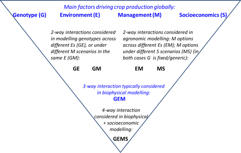
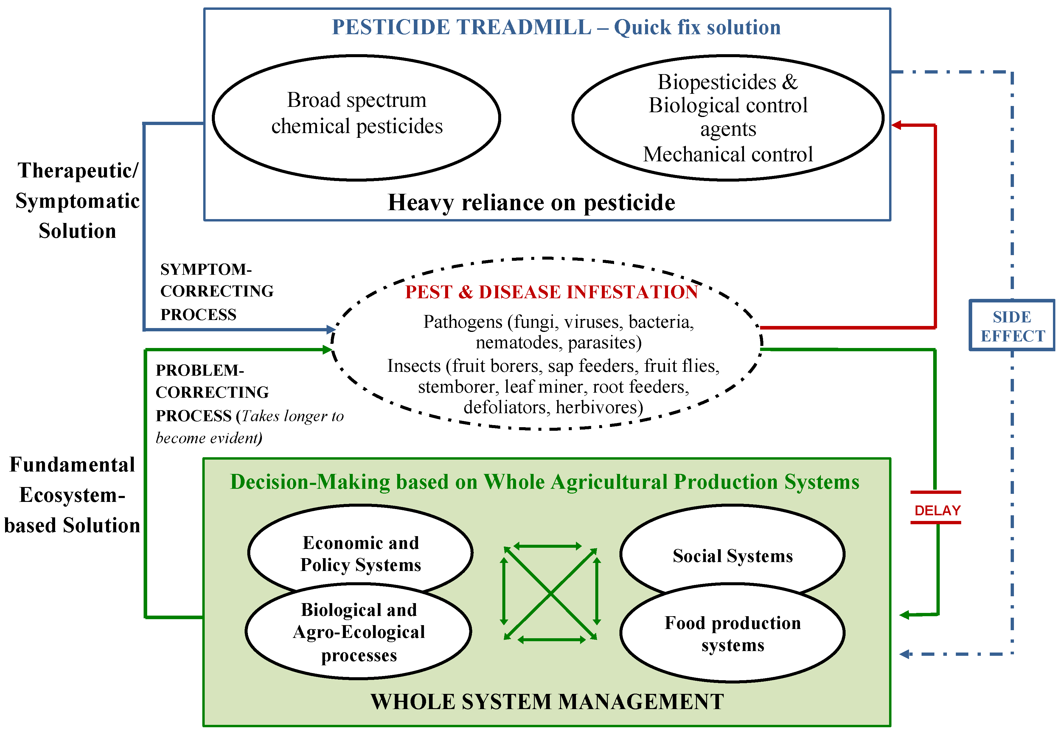
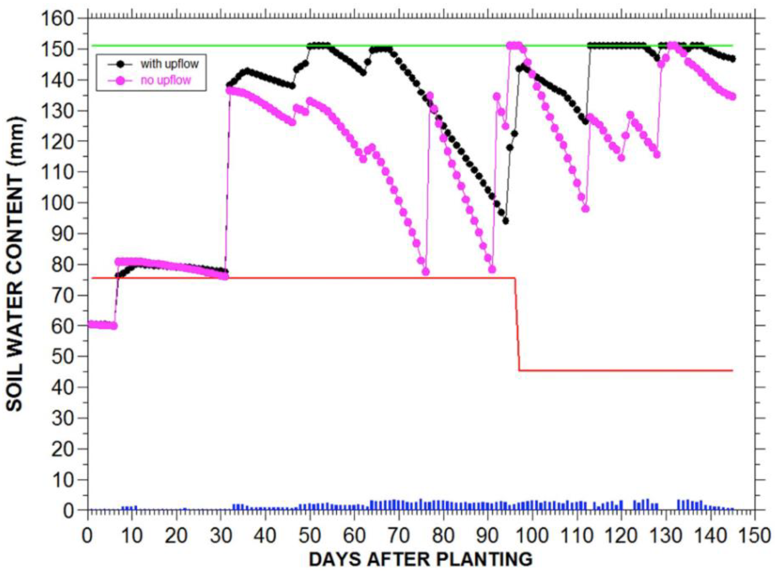
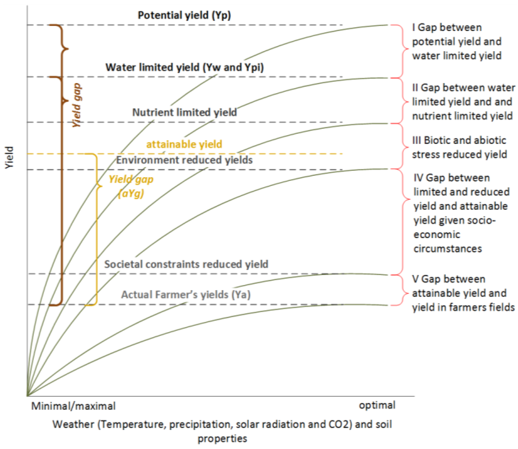
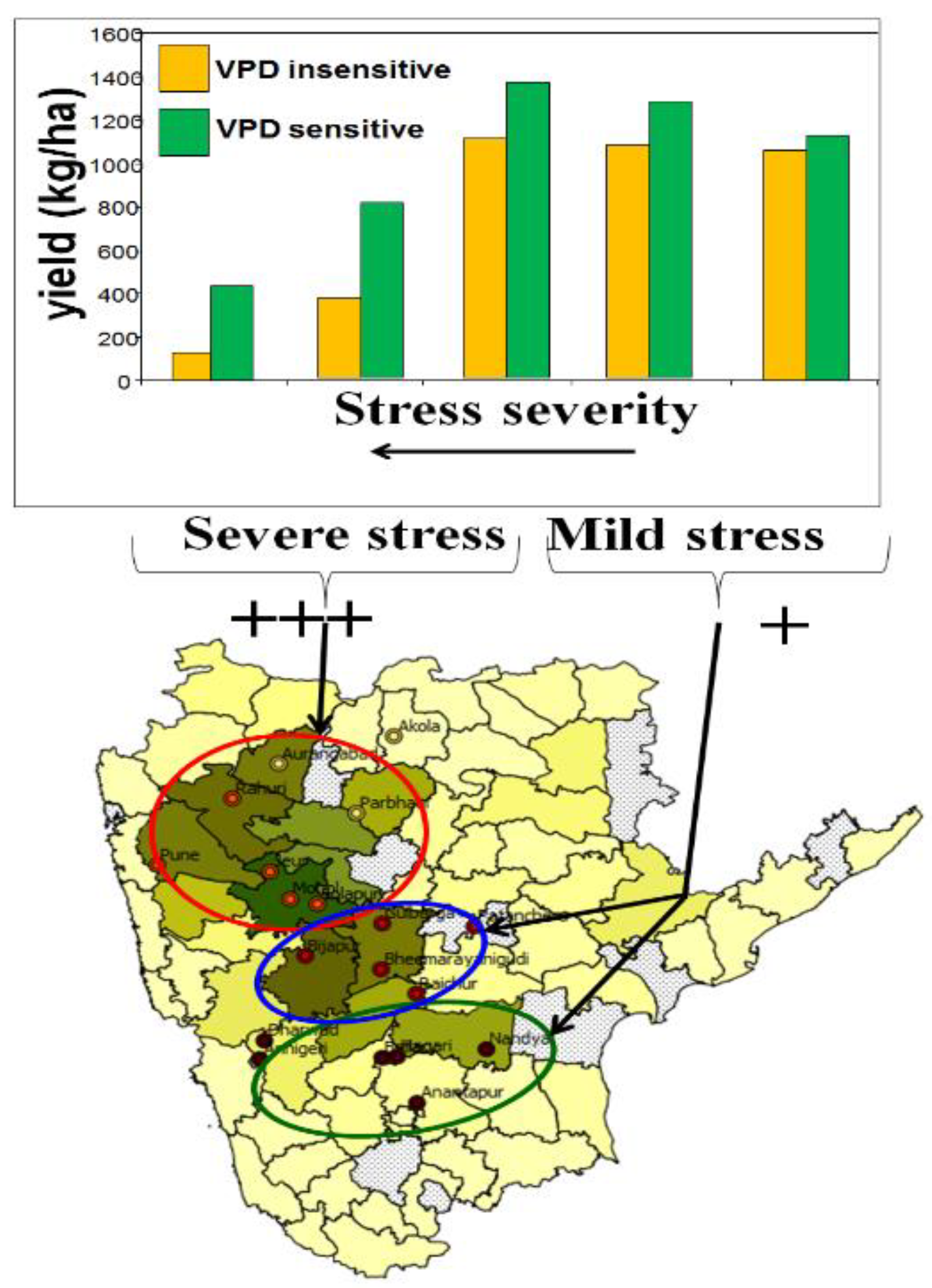
| 1970s FIRST RICE MODELS DEVELOPED | |
| 1980s RICE MODELS | |
| International Rice Research Institute (IRRI): Models developed for rice crops | Whisler, 1983 [15] |
| 1990s FURTHER WORK ON RICE, BEANS, MAIZE | |
| International Rice Research Institute (IRRI): ORYZA model family developed: IRRI, Wageningen UR & National Agricultural Research Systems of 9 Asian countries, Systems Analysis and Simulation in Rice Production (SARP) project. Yield gap analysis, identifying management constraints, climate change analysis, declining yields, Modelling interplant competition (INTERCOM models), Water management optimization, Linking crop and pest models, Plant type design and breeding strategies, Comparing yields in long term trials across years to yield potential, Optimize grain yields with minimum methane emissions, Predict impact of climate change on rice production in Asia using all SARP data | Kropff et al., 1993 [16]; Kropff and Van Laar, 1993 [17]; Kropff et al., 1994 [18]; Wopereis et al., 1994 [19]; Kropff et al., 1995 [20]; Matthews et al., 1995 [21]; Aggarwal et al., 1997 [22]; Kropff et al., 1997 [23]; Teng et al., 1997 [24] |
| West Africa Rice Development Association (WARDA, now known as Africa Rice Center): Rice modeling, model improvement, impact of climate changes in rice yields, genotype by environment | Dingkuhn et al., 1995 [25]; Dingkuhn and Miezan, 1995 [26]; Dingkuhn, 1995 [27]; Dingkuhn 1996 [28]; Dingkuhn and Sow, 1997 [29]; Asch et al., 1997 [30]; Sié et al., 1998 [31,32,33]; Dingkuhn and Asch, 1999 [34] |
| International Crops Research Institute for the Semi-Arid Tropics(ICRISAT): Groundnut modelling | Boote et al., 1992 [35]; Singh et al., 1994 [36]; Singh and Virmani, 1996 [37] |
| International Centre for Tropical Agriculture (CIAT): Bean model development | Hoogenboom et al., 1994 [38]; Hoogenboom et al., 1995 [39]; Acosta-Gallegos et al., 1996 [40] |
| International Maize and Wheat Improvement Centre (CIMMYT): Maize modelling | Elings et al., 1997 [41] |
| 2000s INNOVATIONS IN CROP MODELLING APPROACHES AT CGIAR CENTRES | |
| International Crops Research Institute for the Semi-Arid Tropics (ICRISAT): Crop management, yield gap analysis, analysis of soil constraints and abiotic stress impact for soybean, groundnut and sorghum | Alagarswamy et al., 2000 [42]; Naab et al., 2004 [43]; Bhatia et al., 2006 [44]; Bhatia et al., 2008 [45]; Singh et al., 2009 [46] |
| International Potato Centre (CIP): Growth potential and targeting varieties for potatoes and Andean tubers. Disease modelling for potatoes | Hijmans et al., 2000 [47]; Hijmans, 2003 [48]; Hijmans et al., 2003 [49]; Hijmans et al., 2003 [50]; Andrade-Piedra et al., 2005 [51]; Andrade-Piedra et al., 2005 [52]; Andrade-Piedra et al., 2005 [53]; Condori et al., 2008 [54]; Forbes et al., 2008 [55]; Condori et al., 2010 [56] |
| International Rice Research Institute (IRRI): Further rice model development | Bouman et al., 2001 [57]; Dernier van der Gon et al., 2002 [58]; Kropff et al., 2003 [59] |
| Africa Rice Center (AfricaRice): Intercropping systems, yield gap in rice | Akanvou, 2001 [60]; Haefele et al., 2003 [61]; Akanvou et al., 2006 [62]; van Asten et al., 2003 [63] |
| International Centre for Tropical Agriculture (CIAT): Crop management strategies for dry bean and other tropical legumes | Hartkamp et al., 2002 [64]; Jones and Thornton, 2003 [65]; Jarvis et al., 2008 [66] |
| International Maize and Wheat Improvement Centre (CIMMYT): Modelling for maize and wheat breeding, crop-livestock interactions | Hunt et al., 2003 [67]; Hodson and White, 2007 [68]; Erenstein et al., 2007 [69] |
| International Livestock Research Institute (ILRI): Crop-livestock interactions | Singh et al., 2007 [70]; Erenstein et al., 2007 [69] |
| International Food Policy Research Institute (IFPRI): Impact of climate Change on Agriculture, soil monitoring | Koo et al., 2007 [71]; Nelson et al., 2009 [72] |
| 2010s New interest in global and regional modelling focused on climate change foresight work, strong linkages with AgMIP, modelling groups at UF, CSIRO. Modelling work covering a wide range of uses including agronomy, rotations, agroforestry | |
| CIAT: Climate change impact analysis, including future climates in analogous environments, uncertainties of models and comparisons, abiotic stress testing | Jarvis et al., 2012 [73]; Ramirez-Villegas et al., 2013 [74]; Ramirez-Villegas et al., 2015 [75]; Cammarano et al., 2016 [76]; Eitzinger et al., 2017 [77] Durand et al., 2017 [78]; Ramirez-Villegas et al., 2017 [79]; Piikki et al., 2017 [80]; Fodor et al., 2017 [81]; Heinemann et al., 2017 [82]; Ramirez-Villegas et al., 2018 [83]; Cammarano et al., 2017 [84]; Challinor et al., 2018 [85] |
| IFPRI: Grid-based crop modelling to inform regional and global-scale simulation of food security and international trades under scenarios of agricultural technology developments, food policy, and climate changes | Nelson et al., 2010 [86]; Wiebelt et al., 2013 [87]; Robertson et al., 2013 [88]; Negassa et al., 2013 [89]; Nelson et al., 2014 [90]; Nelson et al., 2014 [91]; Rosegrant et al., 2014 [92]; Muller and Robertson, 2014 [93]; Wiebe et al., 2015 [2]; Robinson et al., 2015 [94]; Robinson et al., 2015 [95]; Islam et al., 2016 [96]; Zougmoré et al., 2017 [97]; Rosegrant et al., 2017 [98]; Rosenzweig et al., 2018 [99] |
| IRRI: Climate change foresight work, genomics studies incorporating crop modelling, abiotic stress modelling, model improvement, improved breeding speed with model assisted selection | Li et al., 2013 [100]; Li et al., 2015 [101]; Li et al., 2015 [102]; Silva et al., 2017 [103]; Dingkuhn et al., 2017a [104]; Dingkuhn et al., 2017b [105]; Mottaleb et al., 2017 [106]; Li et al., 2017 [107]; Savary et al., 2018 [108] |
| CIMMYT: Climate change foresight work on maize and wheat, model improvement, conservation agriculture ex ante modelling, testing of management interventions, Genotype × Environment Interactions | Ngwira et al., 2014 [109]; Chung et al., 2014 [110]; Gbegbelegbe et al., 2014 [111]; Tesfaye et al., 2015 [112]; Tesfaye et al., 2016 [113]; Corbeels et al., 2016 [114]; Rutkoski et al., 2016 [115]; Gaydon et al., 2017 [116]; Aldermann and Stanfill, 2017 [117]; Maiorano et al., 2017 [118]; Tesfaye et al., 2017 [119]; Tesfaye et al., 2017 [120]; Tonnang et al., 2017 [121]; Jain et al., 2017 [122]; Sukumaran et al., 2017 [123]; Sukumaran et al., 2017 [124]; Juliana et al., 2017 [125]; Juliana et al., 2017 [126]; Pérez-Rodríguez et al., 2017 [127]; Montesinos-López et al., 2017 [128]; Montesinos-López et al., 2017 [129]; Montesinos-López et al., 2017 [130]; Sun et al., 2017 [131]; Jarquín et al., 2017 [132]; Dunckel et al., 2017 [133]; Cuevas et al., 2017 [134]; Crossa et al., 2017 [135]; Crespo-Herrera et al., 2017 [136]; Corbeels et al. 2018 [137]; Tesfaye et al., 2018 [138]; Montesinos-López et al., 2018 [139]; Montesinos-López et al., 2018 [140]; Cuevas et al., 2018 [141]; Sukumaran et al., 2018 [142] |
| ICRISAT: Testing genotypes for breeding program orientation, climate change foresight work, drought testing, phenotype evaluations for drought stress, fertilizer response testing, abiotic stress modelling, mixed crop-livestock systems | Vadez et al., 2012 [143]; Singh et al., 2012 [144]; Vadez et al., 2013 [145]; Vadez and Kholova, 2013 [146]; Craufurd et al., 2013 [147]; Nedumaran et al., 2013 [148]; Kholova et al., 2013 [149], Homann-Kee et al., 2013 [150]; Kholova et al., 2014 [151]; Sinclair et al., 2014 [152]; Singh et al., 2014 [153]; Singh et al., 2014 [154]; Singh et al., 2014 [155]; Singh et al., 2014 [156]; Soltani et al., 2016 [157]; Vadez et al., 2017 [158]; Traore et al., 2017 [159]; Singh et al., 2017 [160]; Mohammed et al., 2017a [161]; Mohammed et al., 2017b [162]; Boote et al., 2017 [163]; Nelson et al., 2018 [164]; Faye et al., 2018 [165]; Adam et al., 2018 [166] |
| CIP: Potato disease modelling, foresight, further model development | Kroschel et al., 2013 [167]; Sporleder et al., 2013 [168]; Condori et al., 2014 [169]; Carli et al., 2014 [170]; Kleinwechter et al., 2016 [171]; Kroschel et al., 2017 [172]; Fleisher et al., 2017 [173]; Raymundo et al., 2017 [174]; Raymundo et al., 2017 [175]; Quiroz et al., 2017 [176]; Ramirez et al., 2017 [177]; Mujica et al., 2017 [178]; Scott and Kleinwechter, 2017 [179]; Petsakos et al., 2018 [180] |
| AfricaRice: Model improvement, yield gap analysis, genotype × environment interactions, impact of climate change | van Oort et al., 2014 [181]; van Oort et al., 2015 [182]; van Oort et al., 2015 [183]; Dingkuhn et al., 2015 [184]; van Oort et al., 2016 [185]; El-Namaky and van Oort, 2017 [186]; van Oort et al., 2017 [187]; Dingkuhn et al., 2017 [104,105]; van Oort and Zwart, 2018 [188]; van Oort, 2018 [189], Duku et al., 2018 [190] |
| ICRAF: Agroforestry and intercropping modelling Africa | Luedeling et al., 2014 [191]; Araya et al., 2015 [192]; Luedeling et al., 2016 [193]; Smethurst et al., 2017 [194], Masikati et al., 2017 [195] |
| ILRI: crop-livestock-farm interactions | Van Wijk et al., 2014 [196]; Herrero et al., 2014 [197] |
| IITA: Modelling on Yams in West Africa | Marcos et al., 2011 [198]; Cornet et al., 2015 [199]; Cornet et al., 2016 [200] |
| ICARDA: Climate variability and change impact studies, foresight, conservation agriculture impact, genotype × environment interactions | Sommer et al., 2013 [201]; Bobojonov and Aw-Hassan, 2014 [202]; Dixit and Telleria, 2015 [203]; Frija and Telleria, 2016 [204]; Ghanem et al., 2015 [205]; Ghanem et al., 2015 [206]; Soni et al., 2016 [207]; Mohammed et al. [161], 2017; Dixit et al., 2018 [208]; Mohammadi et al., 2018 [209] |
| Treatments: |
|
| Minimum Dataset to Define Target Environment: |
|
| Trade-Offs | Crop Establishment System | Rice Variety Duration | Rice Sowing | System REY (t ha−1) | Irrigation (mm) | ET (mm) | Deep Drainage (mm) | WPI (kg ha−1 mm−1) | WPET (kg ha−1 mm−1) |
|---|---|---|---|---|---|---|---|---|---|
| Best FP | FP | Long (150 days) | Early June | 13.5 | 1380 | 1270 | 620 | 9.9 | 10.6 |
| Highest productivity | Full CA | Medium (135 days) | Mid-June | 18.0 | 980 | 1360 | 300 | 19.1 | 13.3 |
| Minimum irrigation | Full CA | Short (125 days) | Mid-June | 16.7 | 730 | 1180 | 370 | 23.9 | 14.2 |
| Ground water depletion | Partial CA | Short (125 days) | June and July | 12.0 | 580 | 950 | 380 | 21.7 | 12.5 |
| Society benefit | Full CA | Short (125 days) | Mid-July | 17.2 | 790 | 1160 | 315 | 22.8 | 14.8 |
© 2018 by the authors. Licensee MDPI, Basel, Switzerland. This article is an open access article distributed under the terms and conditions of the Creative Commons Attribution (CC BY) license (http://creativecommons.org/licenses/by/4.0/).
Share and Cite
Reynolds, M.; Kropff, M.; Crossa, J.; Koo, J.; Kruseman, G.; Molero Milan, A.; Rutkoski, J.; Schulthess, U.; Balwinder-Singh; Sonder, K.; et al. Role of Modelling in International Crop Research: Overview and Some Case Studies. Agronomy 2018, 8, 291. https://doi.org/10.3390/agronomy8120291
Reynolds M, Kropff M, Crossa J, Koo J, Kruseman G, Molero Milan A, Rutkoski J, Schulthess U, Balwinder-Singh, Sonder K, et al. Role of Modelling in International Crop Research: Overview and Some Case Studies. Agronomy. 2018; 8(12):291. https://doi.org/10.3390/agronomy8120291
Chicago/Turabian StyleReynolds, Matthew, Martin Kropff, Jose Crossa, Jawoo Koo, Gideon Kruseman, Anabel Molero Milan, Jessica Rutkoski, Urs Schulthess, Balwinder-Singh, Kai Sonder, and et al. 2018. "Role of Modelling in International Crop Research: Overview and Some Case Studies" Agronomy 8, no. 12: 291. https://doi.org/10.3390/agronomy8120291
APA StyleReynolds, M., Kropff, M., Crossa, J., Koo, J., Kruseman, G., Molero Milan, A., Rutkoski, J., Schulthess, U., Balwinder-Singh, Sonder, K., Tonnang, H., & Vadez, V. (2018). Role of Modelling in International Crop Research: Overview and Some Case Studies. Agronomy, 8(12), 291. https://doi.org/10.3390/agronomy8120291