Evaluation of FAO AquaCrop Model for Simulating Rainfed Maize Growth and Yields in Uganda


Abstract
:1. Introduction
2. Materials and Methods
2.1. Description of the Study Area
2.2. Model Input Data
2.3. Description of AquaCrop Model
2.4. Field Data Collection
2.5. Model Evaluation Criterion
3. Results and Discussion
3.1. Canopy Cover
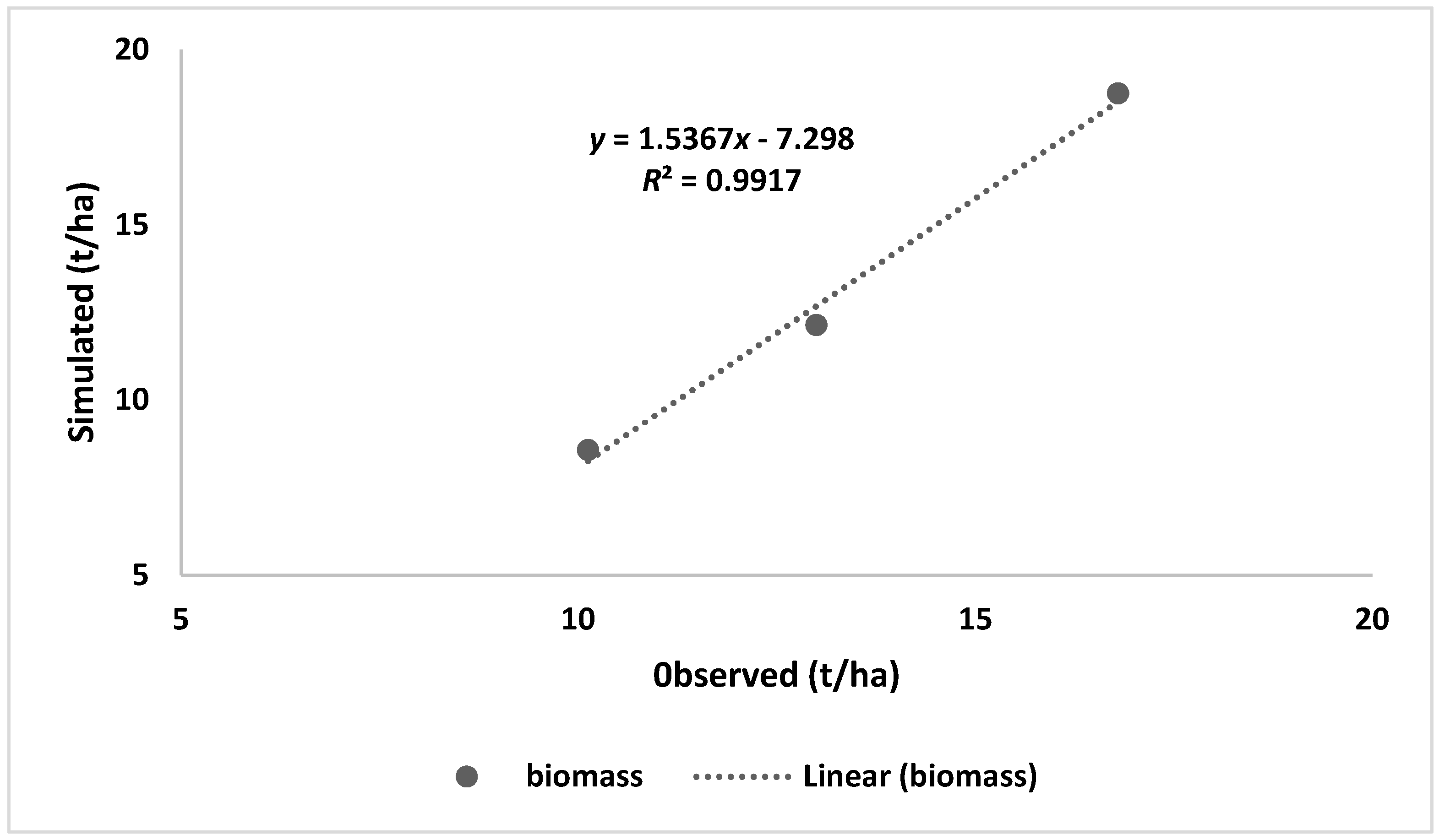
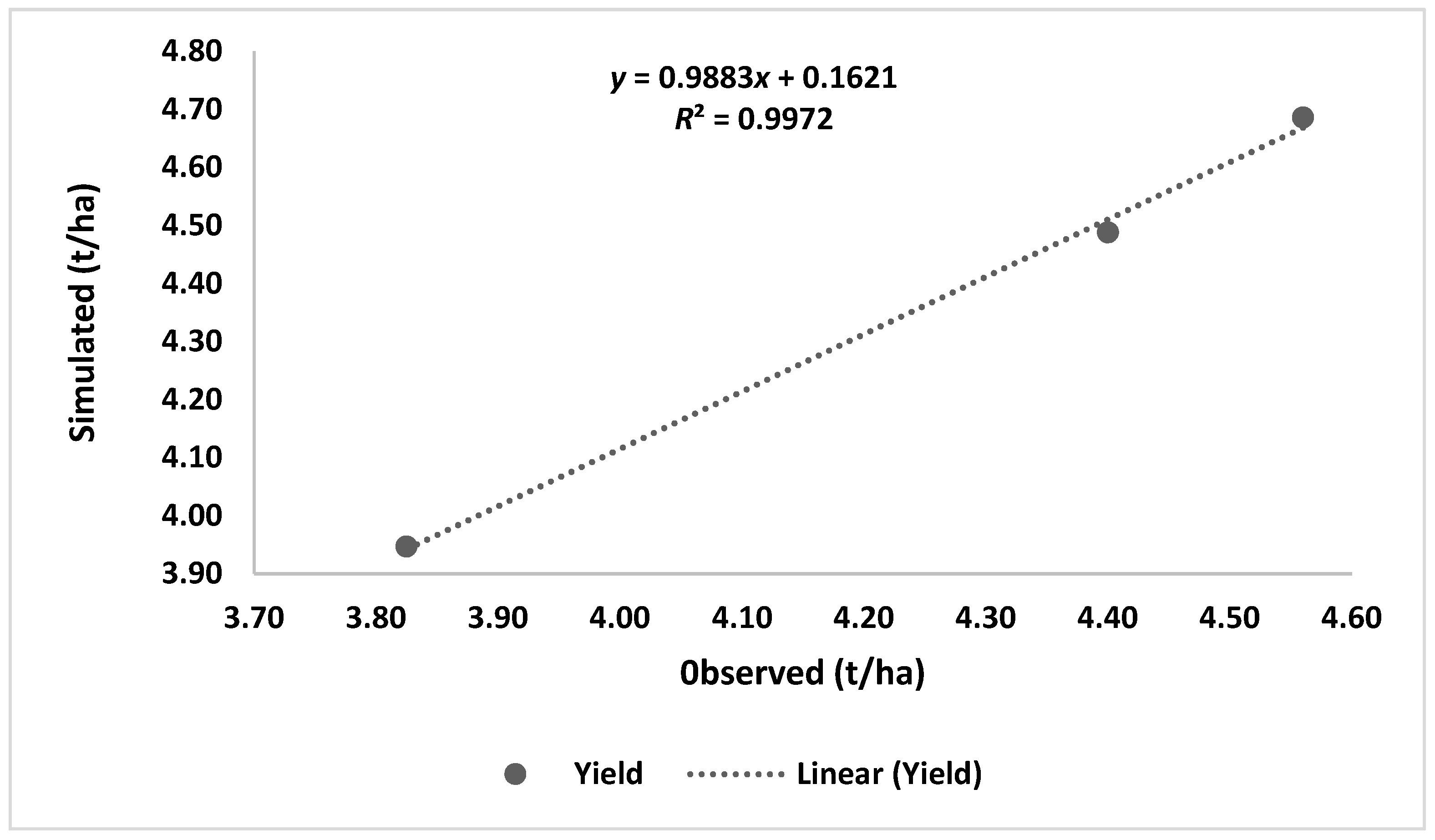
3.2. Final Biomass and Grain Yield
4. Conclusions
Author Contributions
Funding
Conflicts of Interest
References
- UBOS (Uganda Bureau of Statistics). 2016 Statistical Abstract. Uganda Bureau of Statistics. 2016. Available online: http://www.ubos.org/onlinefiles/uploads/ubos/pdf%20documents/abstracts/Statistical%20Abstract%202017.pdf (accessed on 21 August 2017).
- WRMD (Water Resources Management Development). The Year-Book of Water Resources Management Department (WRMD) 2002–2003; Ministry of Water and Environment: Entebbe, Uganda, 2004.
- Rockström, J.; Barron, J. Water productivity in rain fed systems: Overview of challenges and analysis of opportunities in water scarcity prone savannahs. Irrig. Sci. 2007, 25, 299–311. [Google Scholar] [CrossRef]
- USAID (United States Agency for International Development). Uganda Climate Change Vulnerability Assessment Report. African and Latin American Resilience to Climate Change. 2013. Available online: https://www.climatelinks.org/resources/uganda-climate-change-vulnerability-assessment-report (accessed on 21 August 2017).
- Food and Agriculture Organization (FAO). Maize Production in Uganda. Available online: http://www.fao.org/faostat/en/#data/QC (accessed on 19 August 2017).
- UBOS (Uganda Bureau of Statistics). 2013 Statistical Abstract. Uganda Bureau of Statistics. 2013. Available online: http://www.ubos.org/onlinefiles/uploads/ubos/pdf%20documents/abstracts/Statistical%20Abstract%202013.pdf (accessed on 21 August 2017).
- WFP (World Food Programme). Comprehensive Food Security and Vulnerability Analysis. Uganda Bureau of Standards. 2013. Available online: https://documents.wfp.org/stellent/groups/public/documents/ena/wfp256989.pdf?_ga=2.47802279.126176350.1538123855-339799242.1538123855 (accessed on 8 May 2015).
- Republic of Uganda. Uganda’s National Development Plan (2010/11–2014/15). 2010. Available online: http://www.adaptation-undp.org/sites/default/files/downloads/uganda-national_development_plan.pdf (accessed on 19 August 2017).
- McCready, M.S.; Dukes, M.D.; Miller, G.L. Water conservation potential of smart irrigation controllers on St. Augustine grass. Agric. Water Manag. 2009, 96, 1623–1632. [Google Scholar] [CrossRef]
- Kiggundu, N.; Migliaccio, K.W.; Schaffer, B.; Li, Y.; Crane, J.H. Water savings, nutrient leaching, and fruit yield in a young avocado orchard as affected by irrigation and nutrient management. Irrig. sci. 2012, 30, 275–286. [Google Scholar] [CrossRef]
- Mbabazi, D.; Migliaccio, K.W.; Crane, J.H.; Fraisse, C.; Zotarelli, L.; Morgan, K.T.; Kiggundu, N. An irrigation schedule testing model for optimization of the Smartirrigation avocado app. Agric. Water Manag. 2017, 179, 390–400. [Google Scholar] [CrossRef]
- Uganda Bureau of Statistics; Ministry of Agriculture, Animal Industry and Fishers. Uganda Census of Agriculture 2008/09. 2010. Available online: https://www.ubos.org/wp-content/uploads/publications/03_2018UCACrop.pdf (accessed on 10 July 2015).
- Wanga, E.; Robertsona, M.J.; Hammera, G.L.; Carberrya, P.S.; Holzwortha, D.; Meinkea, H.; Chapmanb, S.C.; Hargreavesa, J.N.G.; Hutha, N.I.; McLeana, G. Development of a generic crop model template in the cropping system model, APSIM. Eur. J. Agron. 2002, 18, 121–140. [Google Scholar] [CrossRef]
- Jones, J.W.; Hoogenboom, G.; Porter, C.; Boote, K.; Batchelor, W.; Hunt, L.; Wilkens, P.; Singh, U.; Gijsman, A.; Ritchie, J. The DSSAT cropping system model. Eur. J. Agron. 2003, 18, 235–265. [Google Scholar] [CrossRef]
- Raes, D.; Steduto, P.; Hsiao, T.C.; Fereres, E. Reference Manual: AquaCrop Plug-in Program Version 4.0; FAO (Food and Agriculture Organization): Rome, Italy, 2012. [Google Scholar]
- Doorenbos, J.; Kassam, A.H. Yield response to water. In FAO Irrigation and Drainage Paper; FAO (Food and Agriculture Organization): Rome, Italy, 1979. [Google Scholar]
- Raes, D.; Steduto, P.; Hsiao, T.C.; Fereres, E. AquaCrop—The FAO crop model to simulate yield response to water: II. main algorithms and software description. Agron. J. 2009, 101, 438–447. [Google Scholar] [CrossRef]
- Steduto, P.; Hsiao, T.C.; Raes, D.; Fereres, E. AquaCrop—The FAO crop model to simulate yield response to water: I. concepts and underlying principles. Agron. J. 2009, 101, 426–437. [Google Scholar] [CrossRef]
- Hsiao, T.C.; Heng, L.K.; Steduto, P.; Rojas-Lara, B.; Raes, D.; Fereres, E. AquaCrop—The FAO crop model to simulate yield response to water: III. Parameterization and testing for maize. Agron. J. 2009, 101, 448–459. [Google Scholar] [CrossRef]
- Heng, L.K.; Hsiao, T.C.; Evett, S.R.; Howell, T.A.; Steduto, P. Validating the FAO AquaCrop model for irrigated and water deficient field maize. Agron. J. 2009, 101, 488–498. [Google Scholar] [CrossRef]
- Araya, A.; Habtu, S.; Hadgu, K.M.; Afewerk, K.; Dejene, T. Test of AquaCrop model in simulating biomass and yield of water deficient and irrigated barley (Hordeum vulgare). Agric. Water Manag. 2010, 97, 1838–1846. [Google Scholar] [CrossRef]
- Ngetich, K.F.; Raes, D.; Shisanya, C.A.; Mugwe, J.; Mugendi, D.N.; Diels, J. Calibration and validation of AquaCrop model for maize in sub-humid and semi-arid regions of highlands of Kenya. In Proceedings of the RUFORUM Third Biennial Conference, Entebbe, Uganda, 24–28 September 2012. [Google Scholar]
- Majaliwa, J.G.M.; Omondi, P.; Komutunga, E.; Aribo, L.; Isubikalu, P.; Tenywa, M.M.; Massa-Makuma, H. Regional climate model performance and prediction of seasonal rainfall and surface temperature of Uganda. Afr. Crop Sci. J. 2012, 20, 213–225. [Google Scholar]
- De Groote, H.; Gunaratna, N.S.; Ergano, K.; Friesen, D. Extension and adoption of biofortified crops: Quality protein maize in East Africa. In Proceedings of the 2010 AAAE Third Conference/AEASA 48th Conference, Cape Town, South Africa, 19–23 September 2010. [Google Scholar]
- Allen, R.G.; Pereira, L.S.; Raes, D.; Smith, M. Crop Evapotranspiration-Guidelines for Computing Crop Water Requirements-FAO Irrigation and Drainage Paper 56; FAO (Food and Agriculture Organization): Rome, Italy, 1998. [Google Scholar]
- Food and Agriculture Organization of the United Nations. Eto Calculator; Version 3.1; Evapotranspiration from Reference Surface; FAO (Food and Agriculture Organization), Land and Water Division: Rome, Italy, 2009. [Google Scholar]
- Klute, A.; Dirksen, C. Hydraulic conductivity and diffusivity: Laboratory methods. In Methods of Soil Analysis: Part 1—Physical and Mineralogical Methods; Soil Science Society of America: Fitchburg, WI, USA; American Society of Agronomy: Madison, WI, USA, 1986; pp. 687–734. [Google Scholar]
- Cronshey, R. Urban Hydrology for Small Watersheds; US Department of Agriculture, Soil Conservation Service, Engineering Division: Washington, DC, USA, 1986.
- Ferreira, T.; Rasband, W. ImageJ User Guide. IJ1. 46r. Available online: http://imagej.nih.gov/ij/docs/guide (accessed on 8 May 2015).
- Nash, J.E.; Sutcliffe, J.V. River flow forecasting through conceptual models. I. A discussion of principles. J. Hydrol. 1970, 10, 282–290. [Google Scholar] [CrossRef]
- Mebane, V.J.; Day, R.L.; Hamlett, J.M.; Watson, J.E.; Roth, G.W. Validating the FAO AquaCrop model for rainfed maize in pennsylvania. Agron. J. 2013, 105, 419–427. [Google Scholar] [CrossRef]
- Stricevic, R.; Djurovic, N.; Cosic, M.; Pejic, B. Assessment of the AquaCrop Model in Simulating Rain fed and Supplementally Irrigated Sweet Sorghum Growth; International Commission on Irrigation and Drainage: New Delhi, India, 2011; pp. 201–212. [Google Scholar]
- Brouwer, C.; Heibloem, M. Irrigation Water Management: Training Manual No. 3: Irrigation Water Needs; FAO (Food and Agriculture Organization): Rome, Italy, 1986. [Google Scholar]


| Parameter | September to December 2014 | March to July 2015 | September to December 2015 |
|---|---|---|---|
| Plant population, plants ha−1 | 66,667 | 50,000 | 53,333 |
| Sowing date | 12 September 2014 | 25 March 2015 | 14 September 2015 |
| Harvest date | 24 December 2014 | 09 July 2015 | 29 December 2015 |
| Number of days from sowing to emergence | 7 | 6 | 6 |
| Number of days from sowing to flowering | 73 | 72 | 66 |
| Number of days from sowing to maturity | 104 | 107 | 107 |
| Seasonal rainfall, mm | 542 | 302 | 590 |
| Seasonal reference evaporation, mm | 555 | 519 | 691 |
| Average growing degree days, °C day | 1149 | 1145 | 1321 |
| Depth (cm) | Sand % | Clay % | Silt % | pH | BD (g/cm3) | θpwp (%) | θfc (%) | θsat (%) | Ksat (cm/h) |
|---|---|---|---|---|---|---|---|---|---|
| 0–15 | 33 | 37 | 30 | 5.3 | 1.33 | 19 | 31 | 51 | 0.250 |
| 15–30 | 29 | 45 | 26 | 5.4 | 1.35 | 20 | 32 | 51 | 0.248 |
| 30–45 | 26 | 50 | 24 | 5.5 | 1.35 | 17 | 28 | 45 | 0.205 |
| 45–60 | 25 | 56 | 19 | 5.3 | 1.36 | 16 | 26 | 40 | 0.121 |
| Parameter and Unit | Value |
|---|---|
| Base temperature, °C | 8.0 |
| Upper temperature, °C | 30.0 |
| Soil surface covered by an individual seedling at 90% emergence, (cm2/plant) | 6.5 |
| Canopy growth coefficient (CGC), % increase/day | 13 |
| Canopy decline coefficient (CDC), % decrease/day | 10 |
| Crop determinacy linked with flowering | Yes |
| Excess of potential fruits, % | 50 |
| Shape factor describing root zone expansion | 1.3 |
| Crop coefficient when canopy is complete but prior to senescence | 0.95 |
| Decline in crop coefficient after reaching maximum CC, % decline day−1 | 0.30 |
| Water productivity normalized for ETo and CO2, aWP* (g/m−3) | 33.7 |
| Water productivity normalized for ETo and CO2 during yield formation (as % WP* before yield formation) | 50 |
| Coefficient describing negative impact of stomatal closure during yield formation on Harvest Index | 3.0 |
| Possible increase (%) of Harvest Index due to water stress before flowering | None |
| Coefficient describing positive impact of restricted vegetative growth during yield formation on Harvest Index (HI) | Small |
| Coefficient describing negative impact of stomatal closure during yield formation on Harvest Index (HI) | Strong |
| Maximum possible increase in specified Harvest Index, % | 15 |
| Date | Simulated Canopy (%) | Observed Canopy (%) | Deviation |
|---|---|---|---|
| 30 April | 0.33 | 0.63 | −0.3 |
| 1 May | 24.2 | 37.78 | −13.58 |
| 14 May | 71 | 79.96 | −8.96 |
| 30 May | 77.3 | 80.58 | −3.28 |
| 15 June | 72.9 | 77.98 | −5.08 |
| 9 July | 22.9 | 26.5 | −3.6 |
| Growing Season | Biomass (t/ha) | Grain Yield (t/ha) | ||||
|---|---|---|---|---|---|---|
| Measured | Simulated | Deviation(%) | Measured | Simulated | Deviation (%) | |
| September to December 2014 | 13.00 | 12.14 | −6.6 | 4.40 | 4.49 | 2.0 |
| March to July 2015 | 10.13 | 8.57 | −15.4 | 3.83 | 3.95 | 3.2 |
| September to December 2015 | 16.80 | 18.75 | 11.6 | 4.56 | 4.69 | −2.8 |
| Biomass | Grain Yield | |
|---|---|---|
| RMSE (t/ha) | 1.52 | 0.11 |
| E | 0.69 | 0.87 |
© 2018 by the authors. Licensee MDPI, Basel, Switzerland. This article is an open access article distributed under the terms and conditions of the Creative Commons Attribution (CC BY) license (http://creativecommons.org/licenses/by/4.0/).
Share and Cite
Mibulo, T.; Kiggundu, N. Evaluation of FAO AquaCrop Model for Simulating Rainfed Maize Growth and Yields in Uganda. Agronomy 2018, 8, 238. https://doi.org/10.3390/agronomy8110238
Mibulo T, Kiggundu N. Evaluation of FAO AquaCrop Model for Simulating Rainfed Maize Growth and Yields in Uganda. Agronomy. 2018; 8(11):238. https://doi.org/10.3390/agronomy8110238
Chicago/Turabian StyleMibulo, Tadeo, and Nicholas Kiggundu. 2018. "Evaluation of FAO AquaCrop Model for Simulating Rainfed Maize Growth and Yields in Uganda" Agronomy 8, no. 11: 238. https://doi.org/10.3390/agronomy8110238
APA StyleMibulo, T., & Kiggundu, N. (2018). Evaluation of FAO AquaCrop Model for Simulating Rainfed Maize Growth and Yields in Uganda. Agronomy, 8(11), 238. https://doi.org/10.3390/agronomy8110238