Field-Scale Prediction of Winter Wheat Yield Using Satellite-Derived NDVI

Abstract

This study evaluated the potential of Sentinel-2-derived NDVI (Normalized Difference Vegetation Index) for predicting within-field variability of winter wheat grain yield in central Lithuania during the 2024 growing season. Reliable within-field yield prediction remains challenging in regions with heterogeneous soils and limited region-specific models, particularly in northeastern Europe. Grain yield data were obtained from combine harvesters equipped with GPS yield monitoring across 13 fields with a total area of 283.6 ha. NDVI values were calculated for four half-monthly periods from March to May, corresponding to key phenological stages (from tillering to spike emergence). Spatial and temporal variability in NDVI–yield relationships was observed, with early May consistently showing the strongest correlations (r up to 0.49), particularly in lower-fertility fields, indicating its critical role in yield prediction. Machine learning models (Random Forest, XGBoost, and Deep Neural Networks), along with linear regression, were applied to predict yields based on NDVI from four growth stages. Random Forest achieved the highest predictive accuracy (MAE = 0.951 t/ha), outperforming the other models. The model also showed the highest correlation with observed yields (Pearson r = 0.717), indicating strong agreement between predicted and measured values. Feature importance analysis confirmed NDVI from 1 to 15 May as the most influential predictor across all models. Predicted yield maps closely matched observed patterns, with the largest discrepancies near field edges due to combine harvester effects. These findings highlight the utility of mid-season NDVI for precise estimation of within-field grain yield variability and demonstrate that Random Forest models can effectively capture the NDVI–yield relationship, particularly under heterogeneous field conditions.

1. Introduction

Prediction of crop yield is important across different spatial scales, from the field-scale to the global level [1,2]. Individual crop fields are not uniform in terms of soil properties, which is a major cause of within-field yield variability and underlines the need for precision agriculture solutions [3]. Forecasted yield serves, for example, as a basis for estimating fertilization requirements that account for the nutrients removed with the harvested crop [4]. Therefore, it is essential to obtain yield maps that accurately reflect actual yield variability. Such maps can be generated using combine harvesters equipped with yield monitoring systems and GNSS receivers [5]. However, this approach has certain limitations, as the yield data become available only after harvest. Moreover, many combines are either not equipped with yield monitoring systems or have improperly calibrated sensors [6]. An alternative method for yield prediction involves the use of remote sensing data, such as satellite imagery, which can be applied to forecast crop yields [7,8]. This approach is most commonly used for crops forming a uniform canopy, such as cereals, which are widely cultivated worldwide [9].

The most commonly used satellite imagery for agricultural applications comes from the Sentinel-2 satellites (2A, 2B, 2C) and Landsat 8 and 9 [10,11,12]. This is primarily because data from these satellites are freely available and provide relatively high spatial resolution in the visible and near-infrared spectral ranges. For Sentinel-2, the pixel size is 10 m, whereas for Landsat 8 and 9 it is 30 m. An important advantage of the Sentinel-2 constellation is its shorter revisit time, typically ranging from 2 to 5 days, depending on the region [13,14]. In recent years, numerous studies have investigated the use of Sentinel-2 and Landsat imagery for yield prediction at the scale of individual agricultural fields. These studies cover various crop species, with many focusing on wheat [1,15], which is one of the most important cultivated crops and a major staple food globally.

The primary objective of such studies is typically to assess the relationship between various spectral indices and crop yield and to use these indices for in-season yield prediction as early as possible before harvest [15,16,17]. One of the most commonly used vegetation indices for this purpose is the Normalized Difference Vegetation Index (NDVI), which is calculated based on the reflectance of red and near-infrared light [2,9,18]. Predictive models utilize NDVI values captured during different growth stages. A common research focus is to determine the growth stage at which NDVI shows the strongest correlation with wheat grain yield [1,19].

Various statistical models are used for yield prediction, most commonly linear and nonlinear regression models [20,21]. In recent years, with the advancement of machine learning techniques, models such as Random Forests, neural networks, and others have been increasingly applied [2,22,23]. Such models typically offer advantages over classical statistical approaches when handling many variables and large numbers of observations. One of the most recent systematic literature reviews on crop yield prediction using machine learning is the study by Shawon et al. [23], which is mainly based on publications from 2020 to 2024. The most commonly applied algorithms were Random Forest (35%), Gradient Boosting Trees (26%), Support Vector Machine (25%), and Decision Tree (15%). The most frequently used deep learning algorithms for yield prediction were Convolutional Neural Network (CNN) and Long Short-Term Memory (LSTM). In recent years, there has been a clear shift toward more complex ensemble models such as XGBoost, stacking regression, and hybrid approaches. Random Forest (RF) stands out as the most widely used model, reflecting its popularity and reliability in crop yield prediction.

Since there are no universal models applicable to diverse environmental and agronomic conditions, studies incorporating region-specific data are recommended. In the present study, data from Lithuania (a northeastern European region) were collected for several winter wheat fields, together with NDVI values obtained from Sentinel-2 imagery during the period of intensive wheat growth (March–May). Based on these data, various machine learning models were developed and compared to predict wheat yield at the field scale using NDVI as the predictor.

However, despite the extensive research on NDVI-based yield prediction and the use of machine learning models, several gaps remain in the literature. Many previous studies focus on regions with well-documented agronomic practices and relatively homogeneous environmental conditions, limiting the generalizability of their models. Additionally, most studies either analyze NDVI at a single growth stage or do not systematically compare multiple machine learning algorithms under local conditions. Research specifically targeting the northeastern European context, where winter wheat growth is influenced by unique climatic patterns, soil heterogeneity, and management practices, is still limited.

This study addresses these gaps by collecting region-specific field data from Lithuania, covering multiple winter wheat fields, systematically analyzing NDVI values captured at different growth stages during March–May, and comparing a range of machine learning algorithms, including classical and ensemble methods, to identify the most reliable approach for in-season yield prediction. By focusing on local environmental conditions and performing a comparative evaluation of predictive models, this research provides actionable insights for precision agriculture in northeastern Europe and highlights the importance of region-specific model calibration.

2. Materials and Methods

2.1. Study Area and Data Acquisition

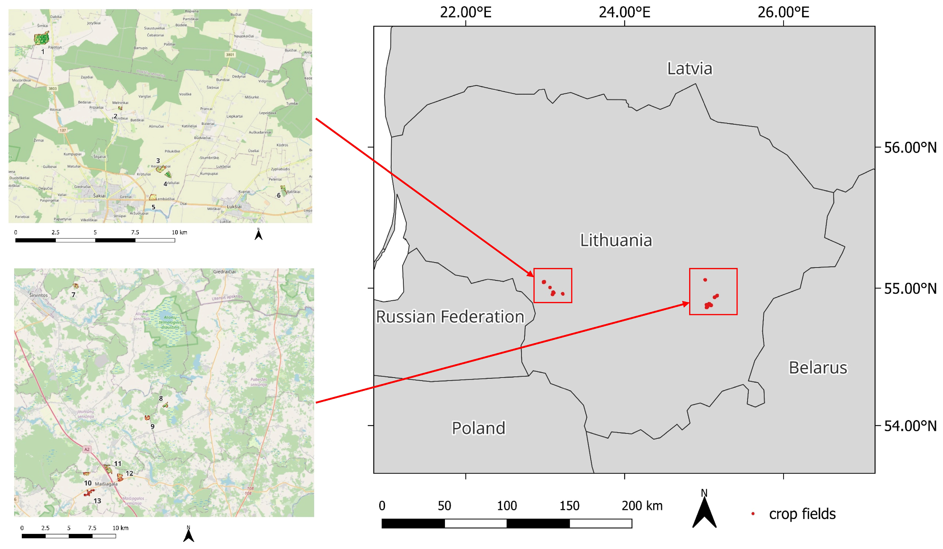
Yield data were acquired from winter wheat fields in central Lithuania between 20 July and 15 August 2024. Thirteen crop fields, ranging in size from 3.91 ha to 58.89 ha, were included in the study (

Table 1. Characteristics of crop fields with winter wheat included in the study, grain yield, and average NDVI for the period March–May 2024.

Crop Field No.	Longitude (° E)	Latitude (° N)	Crop Field Area (in ha)	Sample Size of Yield Data	Grain Yield (t/ha)	NDVI 1–15 May 2024	NDVI 16–30 April 2024	NDVI 1–15 May 2024	NDVI 16–31 May 2024
1	22.98	55.04	58.89	6969	6.84 ± 1.53	0.47	0.66	0.72	0.73
2	23.06	55.00	3.91	643	5.87 ± 1.62	0.57	0.76	0.80	0.80
3	23.10	54.97	15.72	2214	5.81 ± 1.51	0.60	0.73	0.80	0.82
4	23.11	54.97	9.70	1360	6.88 ± 1.35	0.52	0.78	0.84	0.85
5	23.09	54.95	13.83	1918	5.41 ± 0.99	0.28	0.23	0.31	0.48
6	23.22	54.96	7.47	951	5.84 ± 1.62	0.51	0.78	0.81	0.81
7	25.01	55.06	18.81	2797	5.42 ± 1.69	0.44		0.84	0.83
8	25.16	54.95	16.47	2730	6.45 ± 2.11	0.35	0.72	0.83	0.82
9	25.13	54.93	17.54	2066	4.21 ± 1.52	0.38	0.71	0.78
10	25.03	54.88	18.94	3851	5.11 ± 1.74	0.40	0.74	0.85	0.84
11	25.07	54.89	40.82	8224	5.98 ± 1.68	0.33	0.68	0.86	0.89
12	25.09	54.88	34.83	5515	4.53 ± 1.53	0.45	0.82	0.85	0.85
13	25.04	54.86	26.67	4335	3.15 ± 1.32	0.42	0.64	0.75	0.84
Total			283.60	43,573	5.47	0.42	0.69	0.79	0.81

, Figure 1), with a total area of 283.60 ha. After removing outliers (points with zero yield, yields greater than 15 t/ha, and NDVI values below 0.2), the number of sampling points per field ranged from 643 to 6969, with a total of 43,573 sampling points across all fields. Outliers in yield data were identified based on agronomic and regional knowledge. In the conditions of central Lithuania, given local soil types, climate, and typical management practices, wheat yields above 15 t/ha are extremely unlikely and likely represent measurement errors from combine harvesters. Similarly, points with zero yield were considered invalid due to sensor errors or measurements near field edges. Additionally, points with NDVI values below 0.2 were removed to avoid non-vegetated or erroneous measurements. This filtering resulted in the removal of 102 points (0.23% of the total dataset), ensuring that the dataset reflects realistic agronomic conditions while minimizing the influence of erroneous measurements on model training and evaluation.The grain yield data together with NDVI are available in Supplementary Materials (Dataset S1).

Crop fields 1–6 are located near the town of Šakiai (54°57′ N 23°02′ E) in southwestern Lithuania, approximately 60 km west of Kaunas. Fields 7–13 are located near Maišiagala (54°52′ N 25°03′ E) in southeastern Lithuania, about 20 km northwest of Vilnius. Soils in fields 1–6 are classified as Albeluvisols and Luvisols, with topsoil texture classified as loam according to the USDA system (SoilGrids, https://soilgrids.org/ (accessed on 20 January 2026)). In contrast, soils in fields 7–13 are also classified as Albeluvisols and Luvisols but contain a higher proportion of sand and a lower proportion of clay, with sandy loam as the prevailing USDA texture class. Fields 7–13 are characterized by lower soil fertility, and the grain yields obtained in these fields were generally lower than those observed in fields 1–6.

For this study, data from three combine harvesters operating during the 2024 wheat crop harvest were used. The combines were equipped with engines of 320 kW, 370 kW, and 430 kW and featured a telemetry system in which harvest data were automatically recorded and stored. These telemetric systems provide a fully automatic monitoring of harvesting machines under varying weather conditions, crop conditions, grain yields, and moisture levels. The system records numerous operational parameters and performance indicators, which are stored in the onboard microprocessor. The collected telemetry data were exported in Excel format and transferred to a personal computer for further analysis. The recorded parameters included grain yield, grain moisture, travel speed, and other operational variables. Yield monitor data were treated as the reference dataset for yield analysis; however, it should be noted that such measurements may contain uncertainties, particularly near field edges and headlands. In this study, harvesting was conducted using modern combine harvesters equipped with advanced telemetry and yield monitoring systems, which are designed to provide high-resolution and relatively accurate yield measurements under field conditions, although some measurement uncertainty inherent to yield monitor systems may still occur.

The NDVI values were calculated using Sentinel-2 imagery from the COPERNICUS/S2_SR_HARMONIZED (MSI MultiSpectral Instrument, Airbus Defence and Space, Tuluse, France, Level-2A) collection available in Google Earth Engine, as the normalized difference between the near-infrared (B8) and red (B4) spectral bands. To ensure data quality, images affected by cloud cover were excluded, and only pixels classified as vegetation, soil, or water (based on the Scene Classification Layer, SCL) were retained. Mean NDVI values were computed for each yield data point over half-monthly periods and exported to a Google Sheets document for further analysis. Due to cloud cover, it was not possible to obtain NDVI data for the second half of March. Data gaps also occurred in other periods, particularly for fields 7–13 during the first half of April. Therefore, NDVI data from four periods were included in the analyses: 1–15 March 2024 (NDVI-1: end of tillering, BBCH 29); 16–30 April 2024 (NDVI-2: mid stem elongation, BBCH 32–33); 1–15 May 2024 (NDVI-3: late stem elongation, flag leaf visible, BBCH 37–39); and 16–31 May 2024 (NDVI-4: beginning of spike emergence, BBCH 51). The average NDVI values for each period and field are presented in Table 1. As observed, NDVI values increased across successive half-month periods, reaching a maximum at the end of May. The average NDVI across all fields was 0.81, indicating very intense vegetation growth. 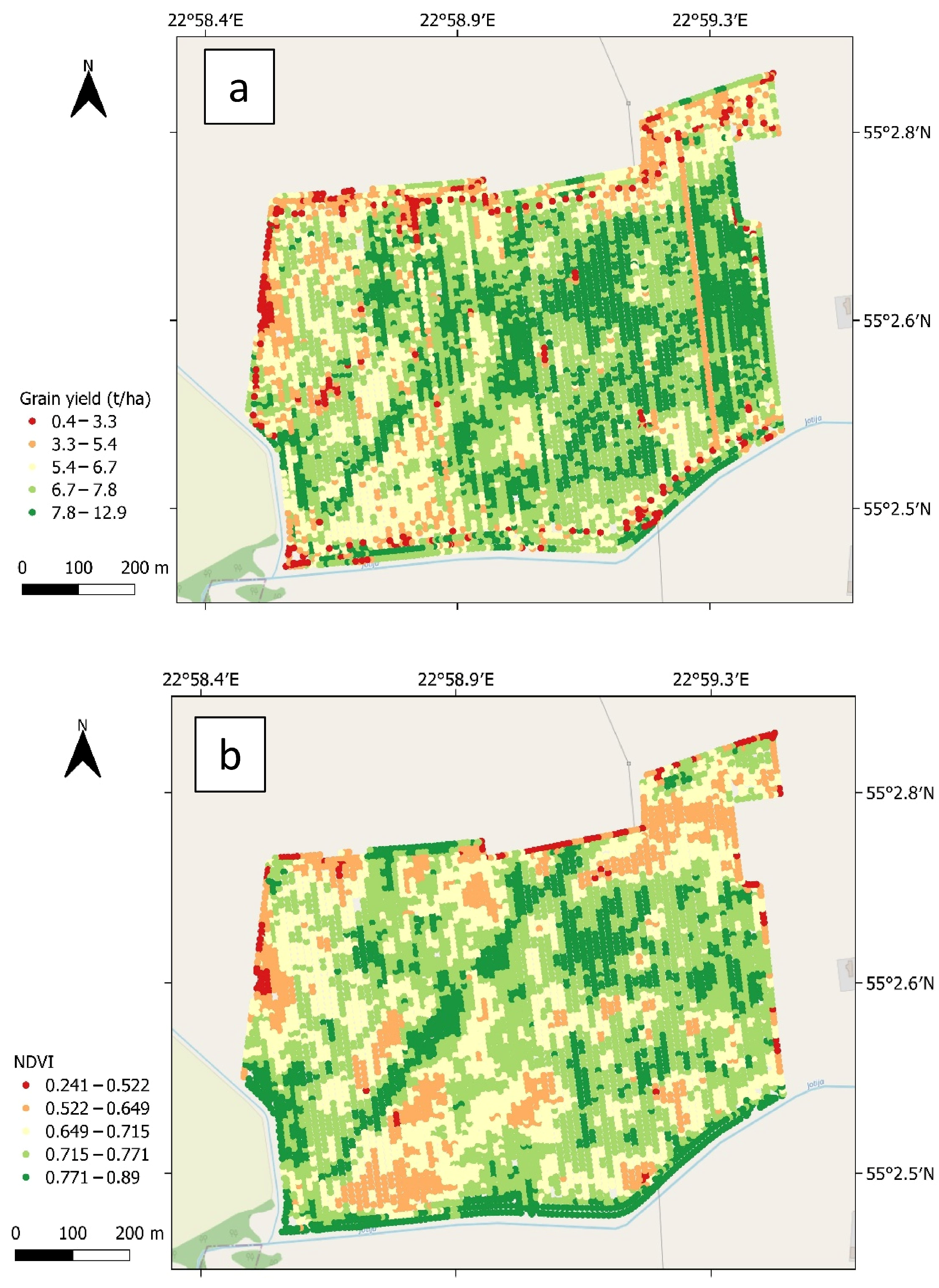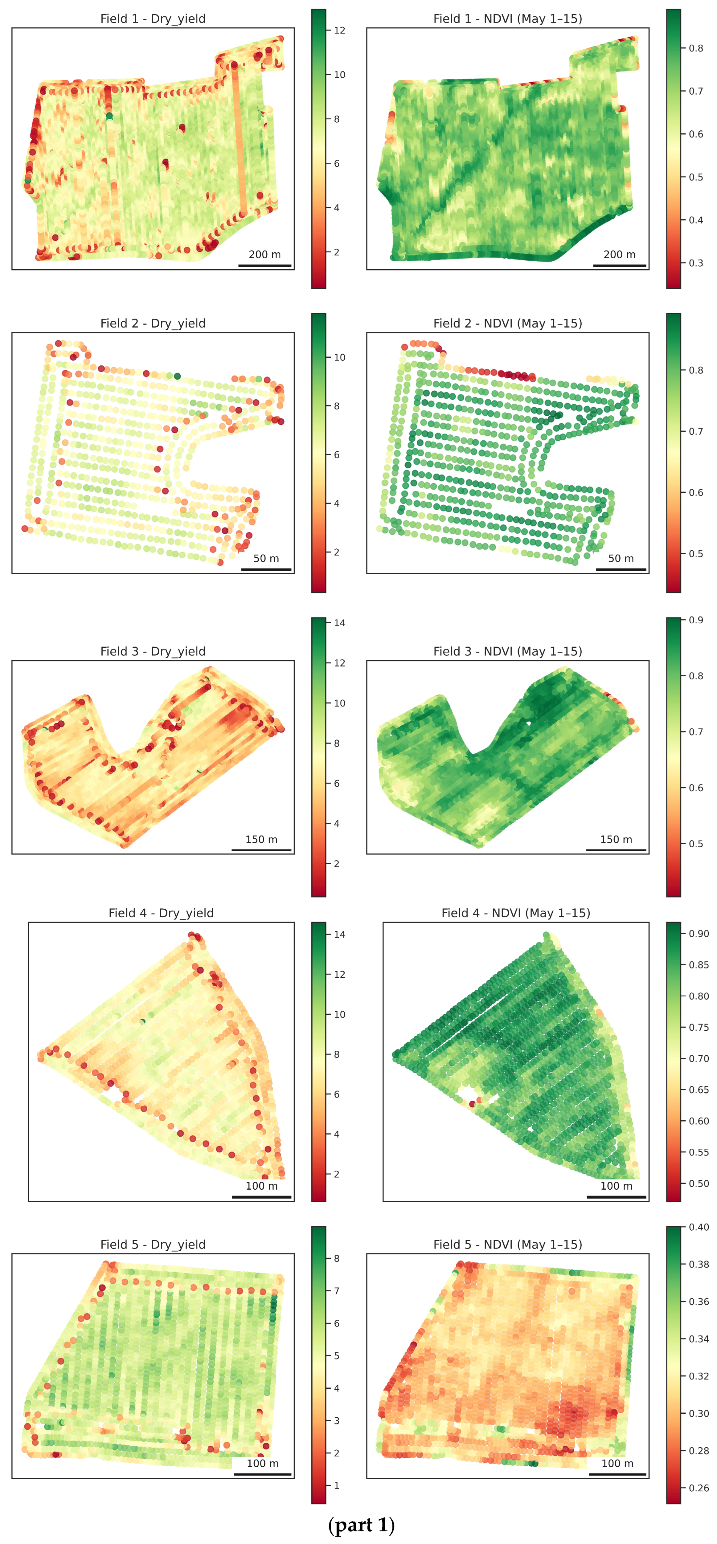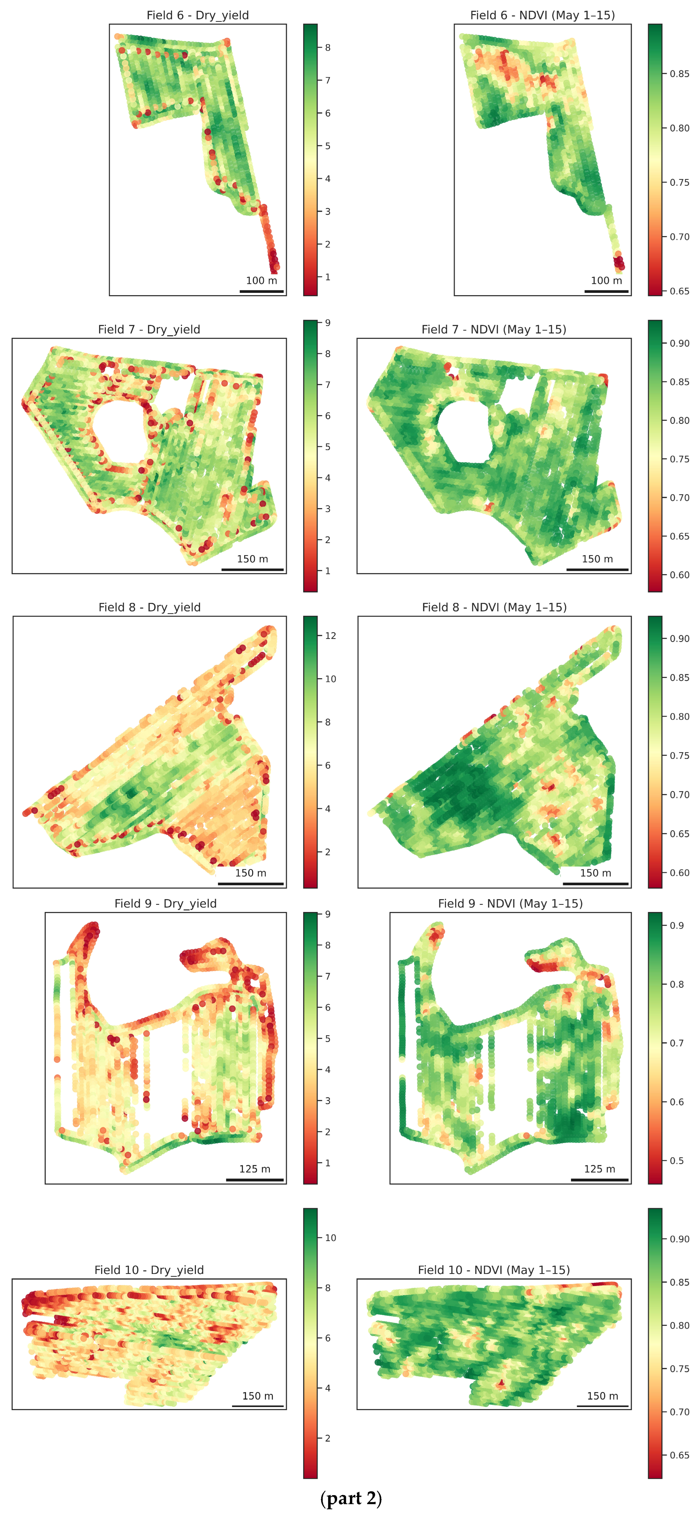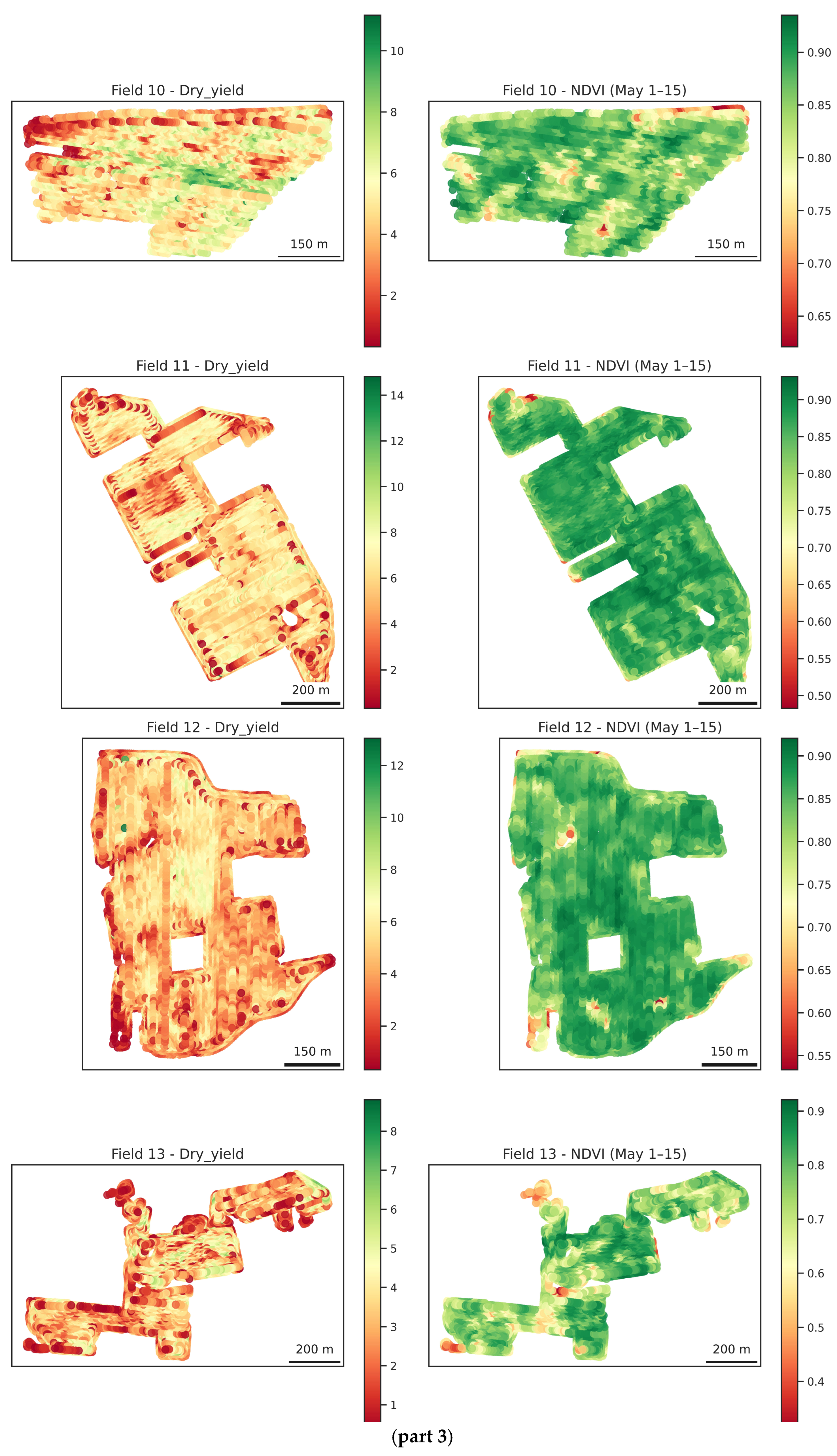Figure 2 presents a grain yield map and the NDVI map for the first half of May for one of the studied fields, while maps for all fields are provided in Figure A1 (Appendix A).

2.2. Data Analysis

Preliminary data preparation was carried out in Microsoft Excel, while geographic data analyses, including the preparation of field maps, were conducted using QGIS version 3.42.

All analyses were performed in Python using the libraries pandas, numpy, scikit-learn, xgboost, statsmodels, and TensorFlow/Keras. Computations were conducted in the cloud-based Google Colaboratory (Colab) environment, which provides a Jupyter notebook interface with preconfigured scientific Python libraries and GPU/CPU computing resources for reproducible machine learning workflows. NDVI values from four half-monthly periods of the 2024 growing season (1–15 March, 16–30 April, 1–15 May, and 16–31 May) were used as predictor variables, while wheat grain yield served as the response variable. Observations with yield values greater than 15 t ha⁻¹ were excluded. Pixels with NDVI values below 0.2 were also removed to avoid non-vegetated or erroneous measurements. Field identifiers were included as additional predictors and encoded using one-hot encoding. The dataset was randomly divided into training (80%) and test (20%) subsets using a fixed random seed (random_state = 42). For the deep neural network model, predictor variables were standardized using z-score normalization.

Random Forest regression was implemented using the RandomForestRegressor algorithm with 300 trees, unrestricted tree depth, and a minimum of two samples per leaf. Gradient boosting was implemented using the XGBRegressor algorithm with 300 boosting iterations, a learning rate of 0.05, maximum tree depth of five, and subsampling of observations and predictors (subsample = 0.8, colsample_bytree = 0.8). The deep neural network was implemented using TensorFlow/Keras as a fully connected feed-forward network with three hidden layers containing 128, 64, and 32 neurons, respectively. LeakyReLU activation functions were applied in hidden layers and dropout regularization (rate = 0.15) was used to reduce overfitting. The network was trained using the Adam optimizer (learning rate = 0.001) and the mean squared error loss function for a maximum of 500 epochs with a batch size of 16. Early stopping with a patience of 30 epochs and learning rate reduction on plateau were applied during training. Twenty percent of the training data was used for validation. Multiple linear regression was implemented using the ordinary least squares method. Model performance was evaluated on the independent test dataset using root mean square error (RMSE) and the coefficient of determination (R²), along with additional diagnostic metrics including mean absolute error, mean absolute percentage error, and Pearson and Spearman correlation coefficients. Feature importance was assessed using model-specific approaches. For Random Forest and XGBoost, feature importance scores were obtained from the trained ensembles. For linear regression, the absolute values of the t-statistics of regression coefficients were used. For the neural network model, permutation importance was applied by measuring the decrease in predictive performance after random shuffling of individual predictors. Importance values were normalized to enable comparison between models.

However, to account for potential spatial autocorrelation within individual fields, we additionally implemented a field-wise cross-validation approach. In this procedure, entire fields were systematically held out as test sets while models were trained on the remaining fields, ensuring spatial independence between training and test data. This field-wise validation was used to verify the robustness of the random splitting approach and assess whether model performance estimates were inflated due to spatial dependence. Comparisons between random splitting and field-wise cross-validation showed consistent results, indicating that the random split provided reliable performance metrics while accounting for spatial structure in the data.

3. Results

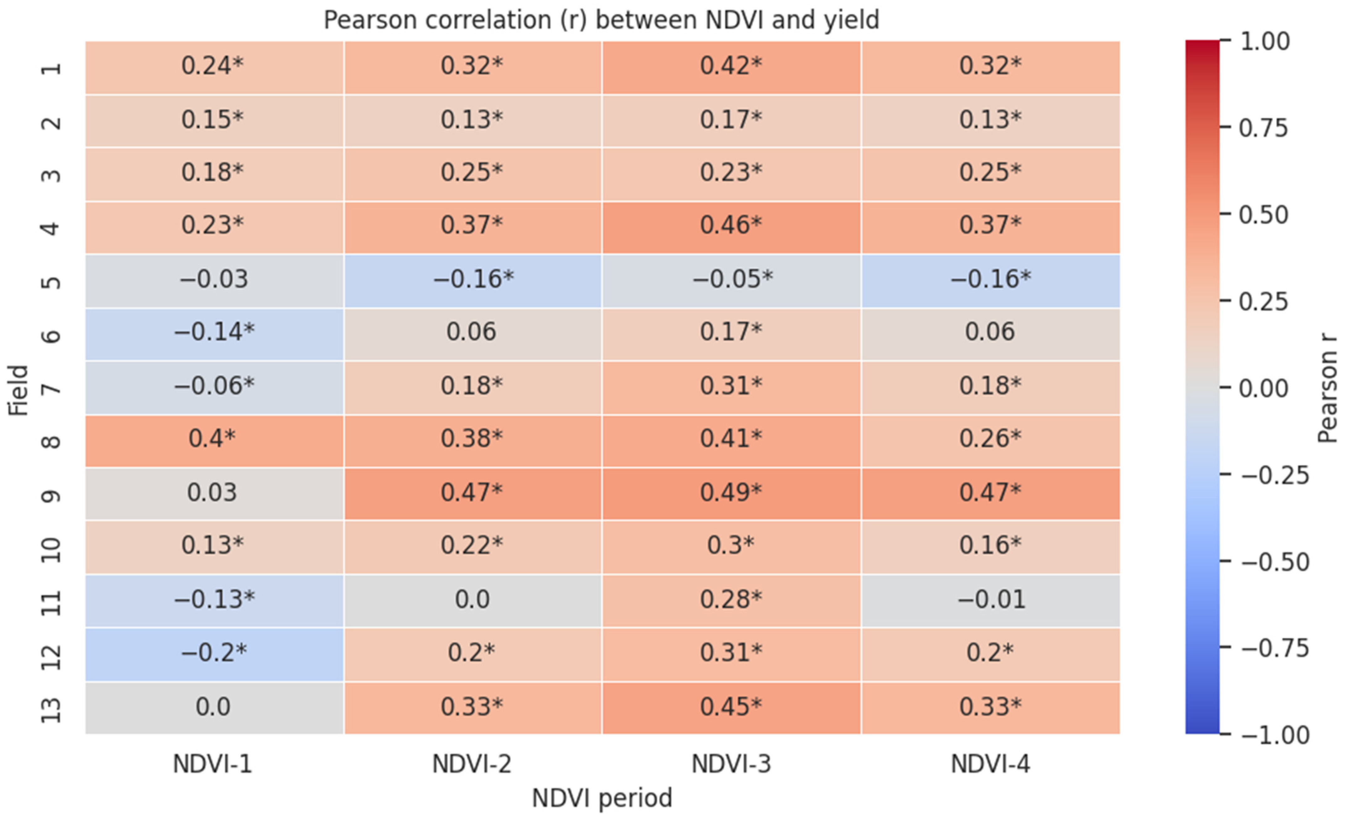
The Pearson correlation coefficients between NDVI values and the studied variable varied across fields and time periods (Figure 3). Overall, correlation strength ranged from weak negative (r = −0.20) to moderate positive (r = 0.49), indicating generally low to moderate association. For most fields, NDVI-3 (1–15 May) showed the highest correlations, suggesting that vegetation status in early May was most closely related to the variable of interest.

The analysis revealed notable spatial and temporal differences in the NDVI–yield relationship. NDVI-3 (1–15 May) consistently produced the strongest correlations in most fields, with the highest values observed in Field 4 (r = 0.462, p < 0.001), Field 9 (r = 0.489, p < 0.001), and Field 13 (r = 0.446, p < 0.001). Fields 5 and 6 exhibited weak or negative correlations in some periods, indicating limited association at any stage. Several fields, including 1, 3, 4, 7, 8, 9, 10, 12, and 13, showed increasing correlations from NDVI-1 to NDVI-3, followed by a plateau or slight decrease at NDVI-4 (16–31 May). Fields 5 and 6 displayed either low or non-significant correlations across all periods, suggesting that early-season NDVI is less predictive of yield in these locations. Fields 7–13, characterized by lower soil fertility, showed higher mean correlations with NDVI than Fields 1–6, particularly at NDVI-2, NDVI-3, and NDVI-4. The difference was most pronounced at NDVI-3, where the mean correlation reached 0.364 for Fields 7–13 compared to 0.233 for Fields 1–6. Overall, the results indicate that early May (NDVI-3) is a key period for monitoring wheat crop performance in central Lithuania, and that the strength of the NDVI–yield relationship is both field-specific and statistically significant in most cases (corresponding p < 0.05).

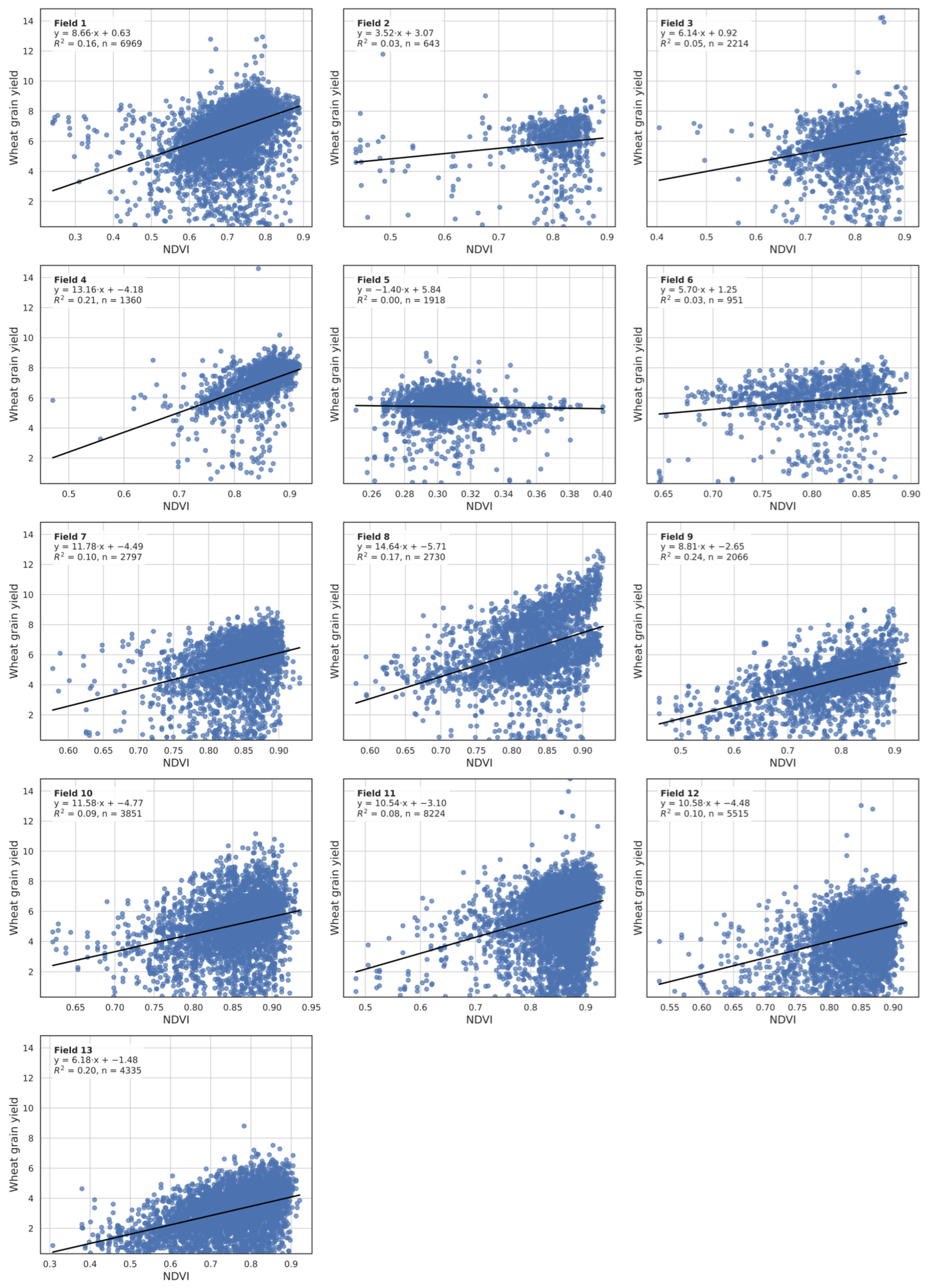
Linear regression results for NDVI-3 (1–15 May) versus dry yield showed substantial variation in the slope coefficient (b) across fields, ranging from −1.397 in Field 5 to 14.639 in Field 8 (Figure 4). Fields with higher b values, such as Fields 4, 8, and 7–10, indicate a stronger positive response of yield to NDVI, whereas Field 5 showed a negligible and slightly negative relationship. Overall, the slope coefficients suggest that NDVI-3 is generally a positive predictor of yield; however, the strength of this relationship varies markedly between fields, with an overall mean b value of 8.45. This indicated that an increase in NDVI of 0.1 corresponds, on average, to an increase in grain yield of approximately 0.85 t/ha. When grouped by fertility and yield, Fields 1–6 showed a lower mean b value of 5.96, while Fields 7–13 exhibited a higher mean b of 10.59, reflecting a stronger NDVI–yield response in the lower-fertility, lower-yield fields.

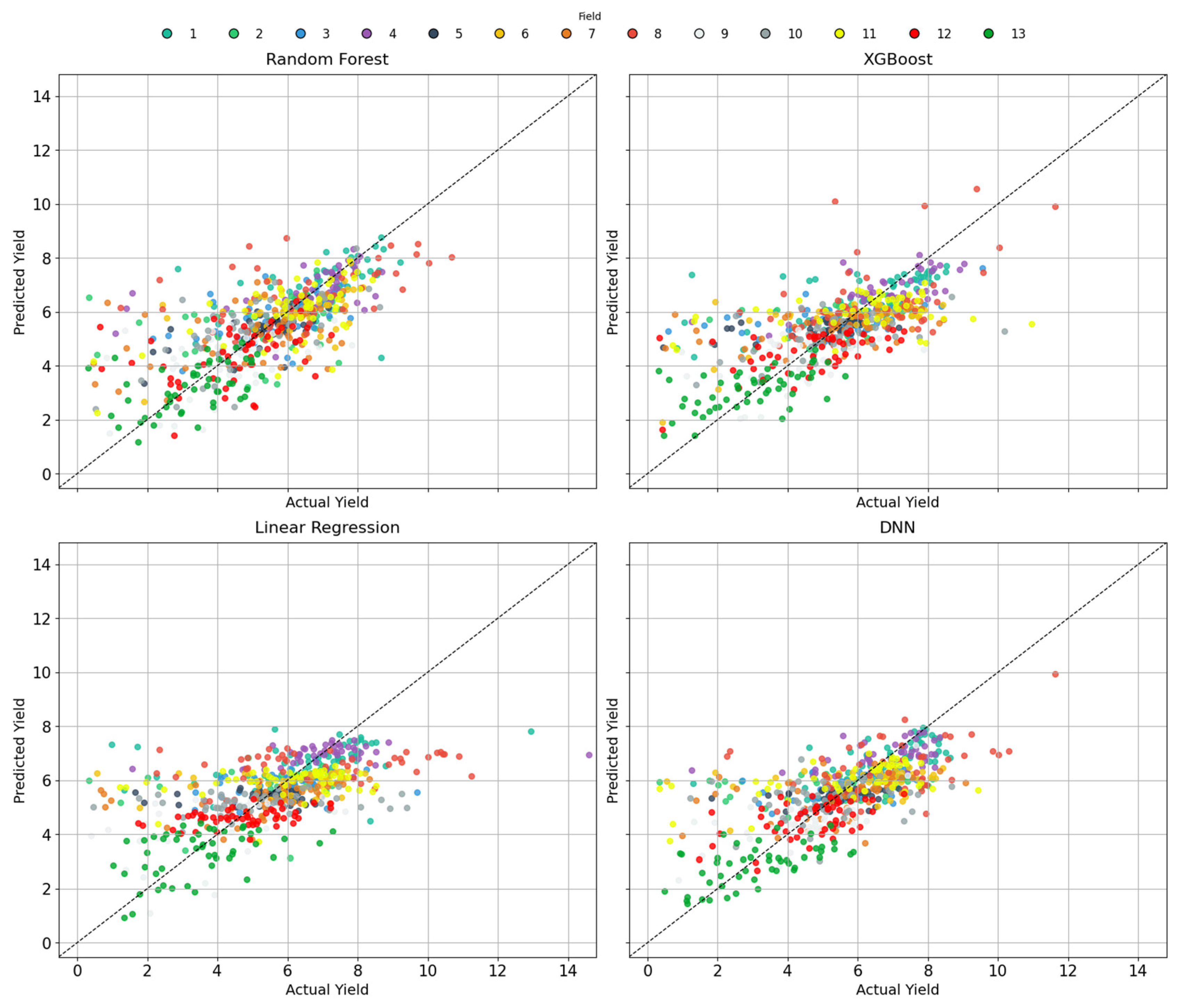
Evaluation of the four models showed that RF achieved the lowest mean absolute error (MAE = 0.951) and mean absolute percentage error (MAPE = 32.54%, as well as the highest Pearson (0.717) and Spearman (0.732) correlation coefficients, indicating the best overall predictive performance (

Table 2. Parameters of accuracy for the models of wheat grain yield prediction based on NDVI for different periods.

Model	Random Forest	XGBoost	Linear Regression	DNN
MAE	0.951	1.028	1.089	1.026
MAPE (%)	32.54	35.77	37.89	35.37
Pearson r	0.717	0.682	0.638	0.681
Spearman ρ	0.732	0.696	0.658	0.694

, Figure 5). XGBoost and DNN produced similar results, with slightly higher errors and marginally lower correlations. In contrast, linear regression showed the weakest performance, with the highest MAE (1.089) and MAPE (37.89%) and the lowest correlation coefficients. Overall, these results suggest that ensemble and neural network models outperform linear regression in capturing the relationship between NDVI and dry yield.

The feature importance analysis revealed that NDVI for 1–15 May (NDVI-3) was the most influential predictor across all models, consistently receiving the highest importance score of 1.00 (

Table 3. Normalized coefficient of importance of predictors for wheat grain yield for different models.

Predictor	RF	XGB	LR	DNN
NDVI 1 March 2024 to 15 March 2024	0.65	0.27	0.29	0.46
NDVI 16 April 2024 to 30 April 2024	0.06	0.00	0.00	0.28
NDVI 1 May 2024 to 15 May 2024	1.00	1.00	1.00	1.00
NDVI 16 May 2024 to 31 May 2024	0.00	0.14	0.08	0.83

). Early-season NDVI (1–15 of March) showed moderate importance in RF and DNN models but much lower influence in XGBoost and linear regression. In contrast, late-season NDVI (16–31 of May) was particularly relevant for the DNN model. Overall, these results indicate that NDVI in early May is the key driver for predicting dry grain yield, whereas NDVI for other periods contributes variably depending on the modelling approach.

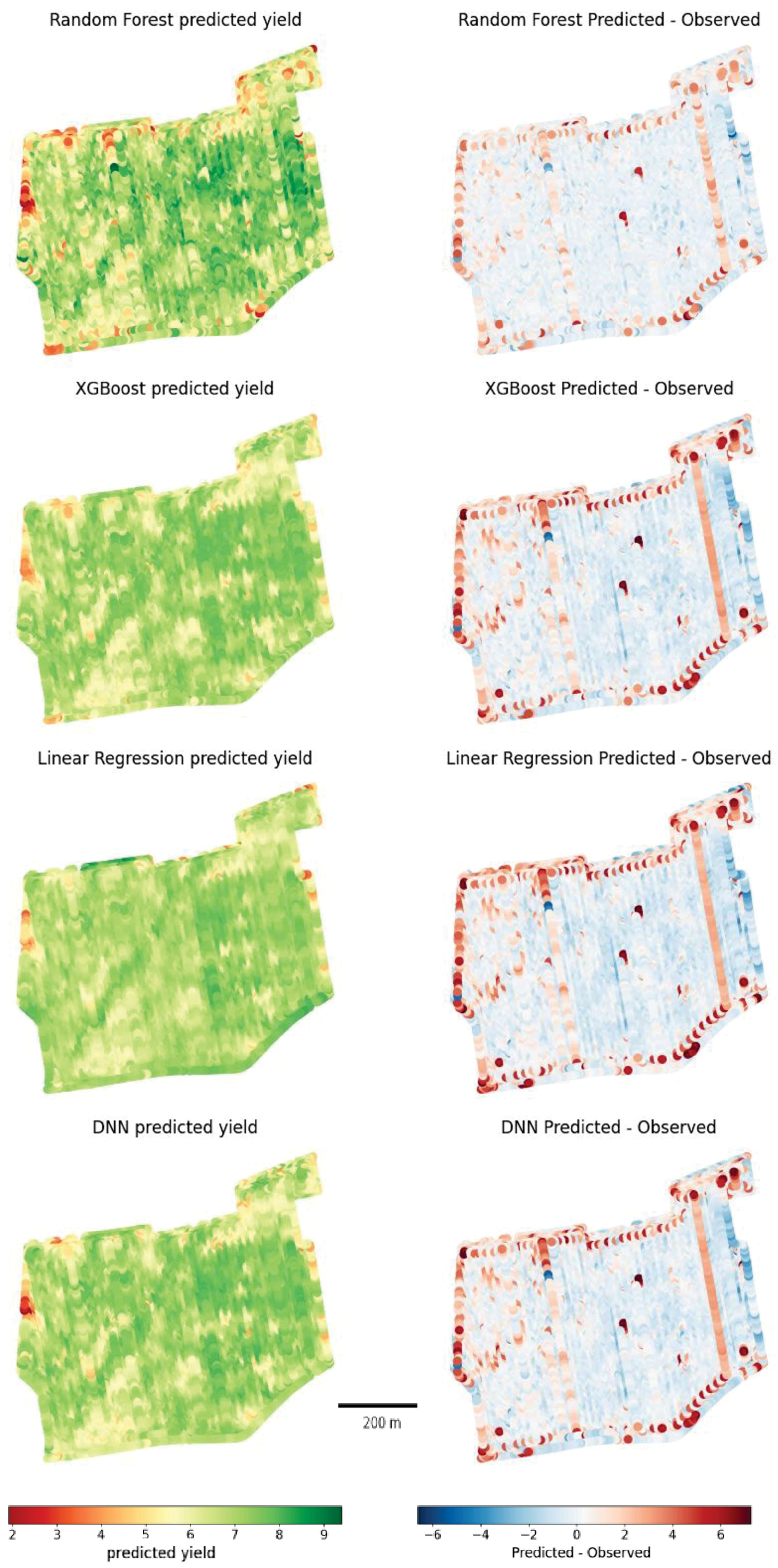
Figure 6 presents maps of predicted yield and a map of prediction errors for one of the studied fields (field no. 1). The special patterns of predicted yields from all four models are consistent with the observed grain yield and NDVI patterns for the first half of May shown in Figure 2. The highest prediction errors were observed near field borders, particularly in combine harvester headland areas. In these zones, predicted grain yield values were often overestimated. Headland yields are likely underestimated by the combine’s yield monitoring system, as the machine enters areas that have already been harvested, resulting in yield measurements that do not reflect actual crop conditions. Therefore, the model-predicted yields in these areas may be more representative of the true yield than the raw combine data.

4. Discussion

The obtained results in this study demonstrate that the relationship between NDVI and wheat grain yield is both temporally and spatially variable. Existing generalized crop yield prediction models are often calibrated using data from regions with relatively homogeneous soils and climate conditions. However, in central Lithuania, winter wheat growth is influenced by spatially variable soil fertility, texture, and local microclimatic factors, which can substantially alter NDVI–yield relationships. This highlights the need for region-specific models, as applying generalized models may lead to under- or overestimation of yield in fields with atypical soil or fertility conditions. Among the analyzed periods, NDVI from 1–15 May (late stem elongation stage, flag leaf visible) showed the strongest and most consistent correlations with yield, indicating that early May represents a critical phenological window for assessing yield potential. Notably, lower-fertility fields (Fields 7–13) consistently exhibited higher NDVI–yield correlations compared to higher-fertility fields (Fields 1–6), particularly during NDVI-2, NDVI-3, and NDVI-4. This pattern suggests that NDVI is more sensitive to yield-limiting factors under less favorable growing conditions, likely reflecting that variability in canopy development due to nutrient or water constraints is better captured in these fields. In contrast, high-fertility fields often showed weaker or negative correlations, possibly due to more uniform canopy cover, reduced variability in yield, or nonlinear responses that simple correlation metrics cannot fully capture.

An additional factor influencing the NDVI–yield relationship is the well-known saturation effect of NDVI at high canopy density. When leaf area index and canopy biomass become high, NDVI tends to approach an asymptotic maximum, which reduces its sensitivity to further increases in vegetation biomass and productivity [24]. This limitation may partly explain the plateau or slight decrease in correlations observed for NDVI-4 (16–31 May), when the wheat canopy was already well developed. Despite this limitation, NDVI was used in the present study because it remains the most widely applied vegetation index in agricultural remote sensing and allows straightforward comparison with numerous previous studies. Sentinel-2 sensors also provide several red-edge bands that enable the calculation of alternative vegetation indices, which are less prone to saturation [25]. However, these red-edge bands are available only at 20 m spatial resolution, whereas the NDVI values used here were derived at 10 m resolution, preserving finer within-field spatial detail. The evaluation of such indices could potentially improve yield prediction accuracy and should be considered in future studies.

Previous studies have shown that the strongest relationships between NDVI and grain yield occur at different growth stages. Segarra et al. [26], in a study on spring wheat in Spain using Sentinel-2 data, demonstrated that NDVI–yield correlations are highly stage-dependent, with the highest correlations observed during the heading stage (r = 0.81). In another field-scale study, Segarra et al. [27] reported that NDVI acquired during stem elongation and flag leaf stages explained a large proportion of wheat yield variability, highlighting the importance of mid-season canopy development for yield estimation. Studies conducted in Iran [28] using Sentinel-2 imagery showed that NDVI–yield relationships strengthened during later vegetative to reproductive stages, while early-season NDVI exhibited weaker and more unstable correlations. In the study by Uribeetxebarria et al. [29] conducted in Spain, the strongest agreement between Sentinel-2 NDVI maps and wheat grain yield maps (Kappa Index > 0.4) was observed after the stem elongation growth stage, although substantial differences were noted between various plots.

Relationships between satellite-derived NDVI and wheat grain variability were often evaluated using Landsat-8 satellite imagery. In the studies of Kaya & Polat [30] and Nagy [31], NDVI derived from Landsat-8 was strongly correlated with wheat grain yield, with the highest correlations typically observed during flowering. In the study of Szabó et al. [32], temporal analyses indicated that the strongest correlation between Landsat-8-derived NDVI and grain yield of wheat was observed during the flowering and fruiting spike period.

In the study of Hassan et al. [33], the strongest relationships were observed for UAV-derived NDVI from early grain filling to late grain filling growth stage. In this study, the relationships were observed under full irrigation and limited irrigation treatments. Much stronger correlations between NDVI and grain yield were observed for full irrigation treatment (maximal correlation coefficient equal 0.77) in comparison to limited irrigation treatments, where correlations were much weaker (maximal correlation coefficient equal 0.37). In the same study, regression analyses evaluating the relationship between NDVI and grain yield were performed separately for each treatment and both treatments together. Values of coefficients of determination were in a very wide range, from 0.04 to 0.89, but were much stronger for regressions evaluated using datasets for both treatments together. Such an effect was because of a wider range of NDVI and a wider range of yields. In our study, a similar effect was observed, because the lowest correlation coefficient (about 0) was observed for field no. 5, where yield variability expressed as standard deviation was the lowest, while for the fields with higher yield variability, the correlation between NDVI and grain yield was usually much higher.

Although the observed correlations between NDVI and wheat grain yield were generally moderate (maximum r = 0.49) and sometimes negative in certain high-fertility fields, this does not undermine the predictive potential of the models. Low correlations in these fields are likely due to limited within-field yield variability, NDVI saturation at high canopy density, local microclimatic effects, and measurement noise near field edges and headlands. Machine learning models, particularly nonlinear ensemble approaches like Random Forest, can capture complex, nonlinear relationships across multiple fields and growth stages, achieving robust predictions even when simple correlations are weak. These results highlight the advantage of ensemble models over linear regression in accounting for field-specific variability. Furthermore, variations in NDVI–yield relationships across fields are explained by differences in soil fertility, texture, water availability, and local microclimatic conditions, emphasizing that predictions are field-specific and sensitive to local environmental factors. In Fields 5 and 6, extremely low or negative correlations are likely a combination of local canopy anomalies, partial NDVI saturation, and potential weed patches or soil reflectance heterogeneity, rather than solely low yield variability, providing a more nuanced explanation than simple standard deviation metrics. Future studies incorporating multi-year and multi-regional datasets could further improve model robustness and generalizability.

Model comparison revealed a clear advantage of nonlinear approaches, particularly Random Forest, over linear regression, highlighting the complex nature of NDVI–yield relationships. Feature importance analysis consistently identified NDVI from early May as the dominant predictor across all models, while the contribution of other periods varied depending on the modelling approach. Spatial analysis of prediction errors showed higher discrepancies near field borders and headland areas, likely due to inaccuracies in combine yield measurements rather than model performance. Overall, these findings confirm the value of early-season remote sensing data for yield prediction and emphasize the importance of accounting for field-specific conditions and data quality in precision agriculture applications.

While Random Forest (RF) achieved the highest predictive accuracy, other models provide useful complementary insights. Linear regression underperformed because it cannot capture nonlinear NDVI–yield relationships or NDVI saturation effects. XGBoost showed slightly lower accuracy, likely due to sensitivity to parameter tuning and smaller sample sizes in some fields. Deep Neural Networks (DNN) require larger datasets to fully exploit spatial and temporal patterns, which were limited at the field scale. This comparison highlights why ensemble and nonlinear approaches outperform simpler models.

Finally, although previous studies report higher NDVI–yield correlations (e.g., r > 0.7–0.8 in Segarra et al. [27], the correlations observed in this study are generally lower (maximum r = 0.49). This is likely due to (i) high-resolution 10 m data capturing micro-scale variability; (ii) higher soil and fertility heterogeneity in central Lithuania; (iii) NDVI saturation in high-fertility fields; and (iv) edge effects and measurement noise. Despite lower raw correlations, nonlinear models like RF are still able to robustly predict yield across heterogeneous fields, demonstrating the practical value of the approach.

Amin et al. [34] developed an operational framework for forecasting within-field grain yield of winter cereals during the growing season using machine learning models based on Sentinel-2 vegetation index time series. Gaussian Process Regression achieved the highest predictive accuracy, particularly when combined with NDVI time series and growing degree days, outperforming Kernel Ridge Regression and RF models. These results demonstrate the strong capability of Gaussian Process Regression to capture nonlinear and temporally continuous crop growth dynamics for yield forecasting ahead of harvest.

Bebie et al. [35] evaluated the potential of Sentinel-2 imagery for predicting durum wheat yield across multiple fields and growing periods, with a focus on early-season yield estimation. Machine learning models, including Random Forest, k-Nearest Neighbors, and boosting regression, consistently outperformed multiple linear regression based on vegetation indices. Notably, Random Forest and k-Nearest Neighbors maintained strong performance even when using images collected up to three months before harvest, highlighting their suitability for early-season within-field yield forecasting.

Recent reviews of machine learning applications in winter wheat yield prediction using vegetation indices such as NDVI and related spectral metrics indicate that nonlinear and ensemble learning methods generally outperform traditional linear regression models in capturing within-field variability [1,36,37,38]. In particular, models such as RF and gradient boosting algorithms have repeatedly demonstrated higher predictive accuracy and robustness across multiple studies, while recurrent and deep learning architectures such as long short-term memory networks have also shown strong performance in accounting for temporal spectral patterns of crop growth. These findings suggest that leveraging advanced ML approaches with Sentinel-2–derived indices substantially improves yield forecasting at the field scale compared to simpler statistical models.

Satellite-derived vegetation indices such as NDVI can complement yield monitor data by reducing noise and spatial inconsistencies caused by sensor calibration and harvesting conditions. In some cases, high-resolution satellite imagery combined with robust modelling approaches can reproduce within-field yield variability with accuracy comparable to harvester-based yield maps. Therefore, satellite data have the potential not only to improve post-processed yield maps but also, under certain conditions, to partially replace yield monitor data in precision agriculture applications [6,39,40]. Such maps can be very useful for optimization of site-specific crop management, e.g., precision variable rate fertilization [41,42].

It should be noted that the present study is limited to a single growing season in central Lithuania. While the results provide valuable insights into the spatio-temporal variability of NDVI–yield relationships and highlight the importance of lower-fertility fields, the findings may not fully represent other years or regions with different soil types, climate conditions, or management practices. Expanding this research to include multi-year and multi-regional datasets would allow a more comprehensive assessment of the robustness and generalizability of NDVI-based yield prediction models. Future studies could also explore the integration of additional remote sensing indices, higher temporal resolution data, and complementary environmental variables to improve predictive performance across diverse agro-ecological contexts.

Furthermore, the observed higher prediction errors at field boundaries suggest that edge-related noise and combine harvester effects influence model accuracy. Implementing a buffer analysis by excluding 10–20 m from field edges could help assess whether predictions improve in these zones. However, in smaller fields, such exclusion would reduce sample size and may affect model representativeness. Future work should investigate edge buffering or smoothing approaches to mitigate boundary-related errors.

Practical application of the proposed NDVI-based yield prediction models lies primarily in within-field precision agriculture and early-season management. By integrating model outputs with farm management systems, farmers can make informed decisions on variable-rate fertilization, targeted irrigation, or other input adjustments based on predicted spatial yield variability. Operationally, this requires acquiring NDVI data at key growth stages (e.g., early May), preprocessing to correct for outliers and noise, and applying the trained models to generate field-scale predictions. Such an approach can improve resource use efficiency, reduce yield variability, and complement traditional yield monitoring methods. Although this study focused on a single growing season and region, the framework demonstrates how remote sensing and machine learning can be translated into actionable management strategies in precision agriculture.

5. Conclusions

This study demonstrates that NDVI derived from the first half of May is a robust and consistent indicator of wheat grain yield across fields with contrasting fertility levels. Yield–NDVI relationships were stronger in lower-fertility fields, highlighting the greater sensitivity of crop spectral response under yield-limiting conditions. Among the tested models, RF provided the highest prediction accuracy, confirming the advantage of nonlinear approaches for modelling NDVI–yield relationships. These findings support the use of early May NDVI for evaluating within-field wheat grain yield variability and spatial yield mapping in precision agriculture, while acknowledging that predictive performance may vary across fields and that further studies could extend the approach to other crops and regions.