TCN-Attention Model-Based Prediction of Reference Crop Evapotranspiration in Northern Henan Province

Abstract

Accurate and reliable estimation of reference crop evapotranspiration (ET₀) in the North Henan Plain is crucial for agricultural water resource management, production, and food supply in China. This study aims to evaluate the performance of deep learning (DL) methods in ET₀ estimation and assess the applicability of the developed DL model beyond the training domain. This study utilized historical meteorological data from Zhengzhou City, northern Henan, spanning 2010–2024. Meteorological variables were selected through correlation analysis and maximum information coefficient (MIC). A novel DL model—the TCN-Attention model (TA)—was constructed by incorporating a self-attention mechanism into the temporal convolutional network (TCN) model. This model was compared with two classical DL models—Long Short-Term Memory (LSTM) and TCN. Results indicate: (1) Sunshine duration ($n$), relative humidity ($\mathrm{R}\mathrm{H}$), and maximum temperature (T_max) are the three most significant features influencing summer maize evapotranspiration; (2) prediction accuracy under the same input scenarios: TA model > TCN model > LSTM model; (3) in scenarios where only temperature data is input, the TA model has the highest prediction accuracy, surpassing the H-S empirical method; and (4) for limited meteorological data, the combination of temperature and humidity was found to be most effective, showing good adaptability and accuracy at different time steps (hourly: R² = 0.982; daily: R² = 0.975; weekly: R² = 0.928). This study highlights the potential of the TA model for estimating reference crop evapotranspiration in the northern Henan Plain, which may provide theoretical guidance for crop irrigation management under future climate change.

1. Introduction

In the context of global water shortages, rational water resource utilization, precision irrigation, and ensuring food production security have become critical for sustainable agricultural development [1]. Water resource management, hydrological research, irrigation scheduling, and crop modelling studies require the calculation of evapotranspiration (ET). Its accurate prediction is a key indicator for measuring crop water demand and formulating an irrigation plan [2,3]. Reference crop evapotranspiration, serving as the fundamental basis for calculating ET, plays vital roles across multiple domains due to its high sensitivity to climate change. These include establishing watershed water balance models, optimizing irrigation system design and management, accurately forecasting crop yields, and rationally allocating water resources in flood and drought risk planning and management [4,5]. Therefore, accurately estimating ET₀ is crucial for ensuring sustainable agricultural practices and effective water conservation strategies [6,7]. Currently, ET₀ can be determined through either direct measurement or mathematical modelling. While direct measurement provides accurate ET₀ data, this method is labour-intensive, costly, and technically complex, limiting its practical applicability [8]. Mathematical modelling estimates ET₀ by establishing equations linking ET₀ to meteorological variables, requiring minimal effort and straightforward calculations [9]. Among these, the most widely adopted globally is the FAO reference crop evapotranspiration model (P-M) proposed by the Food and Agriculture Organization of the United Nations [10], which FAO has recommended as the standard method for calculating ET₀. However, the P-M model involves complex calculations and requires extensive meteorological data, significantly limiting its applicability in regions with insufficient meteorological records [11,12]. Therefore, there is an urgent need to explore a simpler, more efficient, and less meteorologically dependent method to meet irrigation demands in the northern plains of Henan Province and further enhance agricultural water use efficiency.

In recent years, with the rapid development of computer technology, big data, and machine learning algorithms, the application of machine learning algorithms in calculating ET₀ has undergone significant enhancements [13]. A series of typical machine learning models, such as Extreme Gradient Boosting (XGBoost) [14], Support Vector Machines (SVM) [15], and ARIMA models [16], have been widely applied in hydrological modelling. However, traditional machine learning models exhibit limitations when handling complex nonlinear relationships and time series data, leading to a sharp decline in predictive performance [17]. Consequently, many researchers have turned to deep neural networks to enhance the accuracy of ET₀ predictions. Xie Jiaxing et al. [18] conducted a study using meteorological data from citrus orchards in Wuzhou City, Guangxi. Results indicated that the LSTM evapotranspiration model delivered optimal performance in terms of MAE and RMSE, effectively capturing the complex nonlinear relationships between meteorological factors and evapotranspiration. Thus, this model is ideal for formulating irrigation strategies in citrus orchards. Li et al. [19] found that models based on improved convolutional neural networks (CNNs) and LSTMs effectively enhance the accuracy of ET₀ predictions in Northeast China. Yin et al. [20] discovered that Bi-LSTM models can fully utilize limited meteorological data to effectively capture bidirectional dependencies in time series, thereby enhancing the prediction accuracy of $\mathrm{E}{\mathrm{T}}_0$. Although classical LSTM models have been widely applied in hydrological estimation, researchers strive to improve neural network learning capabilities to extract features from meteorological factors [21]. An example is the TCN proposed by Lea et al. [22], designed for forecasting tasks due to its large receptive field and robust feature learning capacity. Chen et al. [23] applied the TCN model to study potential evapotranspiration in Shenyang’s irrigation districts, in China, finding consistent prediction performance across varying input parameters. Gao et al. [24] demonstrated that their TCN model, trained on Dong Lai Yellow River irrigation district data, could accurately predict ET₀ up to 10 days in advance. Ren et al. [25] compared 12 reference evapotranspiration estimation models in Shandong Province, finding that the TCN model delivered the highest accuracy. Additionally, Dong et al. [26,27] discovered that integrating attention mechanisms into deep learning models enhances generalization capability and prediction accuracy.

Based on meteorological data from the Agricultural Hydraulic Research Station of North China University of Water Resources and Electric Power in Zhengzhou, China, this article presents a selection performed using correlation analysis and the maximum information coefficient (MIC) [28]. This study proposes the TA model as an innovative way to estimate ET₀. Simultaneously, the predictive potential of the TA, TCN, and LSTM models was evaluated under different meteorological conditions. The primary objectives of this study are: (1) to develop three DL models—TA, TCN, and LSTM—for predicting $\mathrm{E}{\mathrm{T}}_0$ in the northern Henan Province, China; (2) to compare the estimation performance of the three DL models under limited meteorological data conditions; and (3) to conduct model prediction analysis at different time scales for the optimal model.

2. Materials and Methods

2.1. Overview of the Study Area and Data Sources

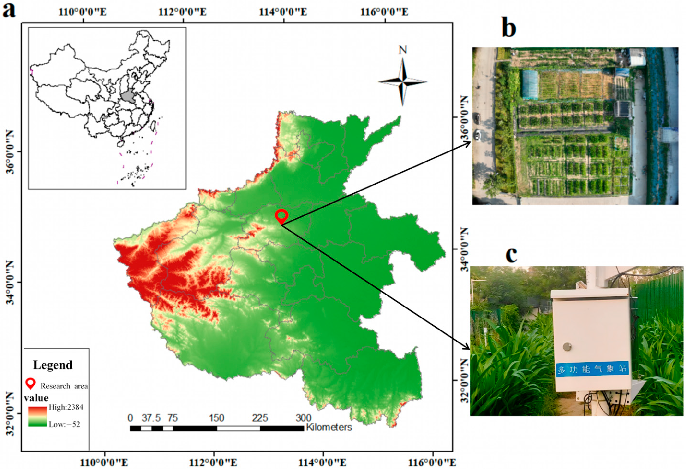
The data for this study come from the Agricultural Water Conservancy Experimental Research Area of North China University of Water Resources and Electric Power in Zhengzhou, Henan Province. This area is located in the northern Henan Plain in the western part of the Huang-Huai-Hai Plain, with an average elevation of about 108 m. The overall terrain is flat with gentle slopes. The research area has a typical warm temperate continental monsoon climate, with distinct seasons, dry winters and springs, and rainy summers. The annual average precipitation is about 600–700 mm, unevenly distributed throughout the year, with more than 50% occurring in July and August. The annual sunshine duration is approximately 2200–2400 h, with light and temperature conditions sufficient to meet the full growth requirements of medium- and late-maturing maize. The northern Henan region, located in the Huang-Huai-Hai Plain, is China’s largest concentrated maize production area. The summer maize growing season coincides closely with periods of heat and rainfall, facing dual risks of seasonal drought and waterlogging during its growth. Therefore, conducting research on the reference crop evapotranspiration of summer maize in this region and accurately predicting its water needs is not only a key agronomic issue for improving crop yield and water use efficiency, but also an important macro-level topic related to China’s food security strategy, sustainable agricultural economic development, and climate change adaptation. The location and field conditions of the research area are shown in Figure 1.

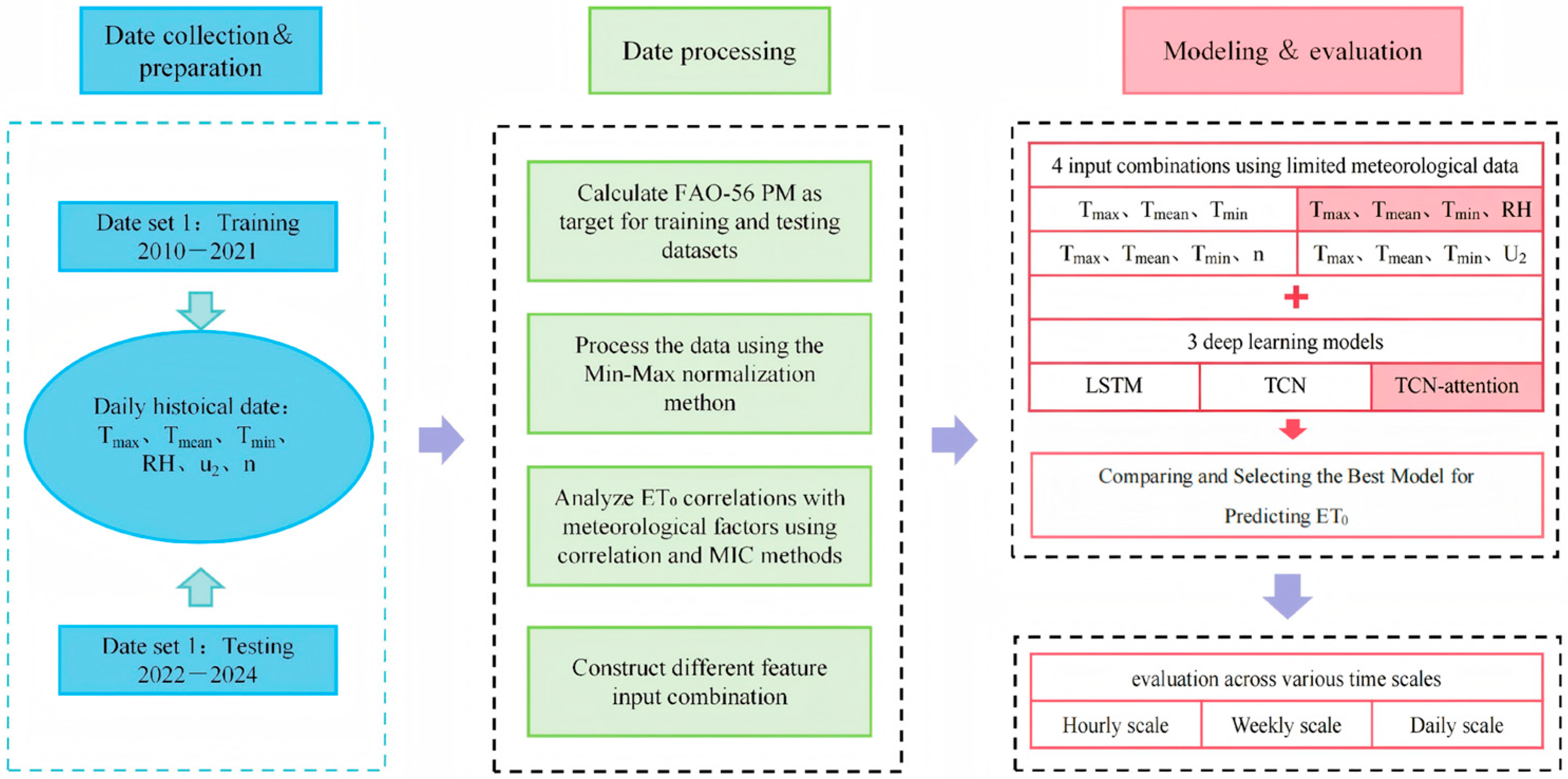
Meteorological dataset from 15 June 2010 to 30 September 2024, consisting of daily meteorological data at weather stations during the growing season of summer maize, including daily maximum temperature (T_max), daily minimum temperature (T_min), daily mean temperature (T_mean), 2 m above ground wind speed (U₂), relative humidity (RH), and sunshine duration (n), are all recorded hourly using the STQ-1 portable mobile mini automatic weather station(manufacturer: Stark IoT Technology Co., Ltd.; location of procurement: Handan City, Hebei Province, China). These data were recorded from 10 June 2018 to 30 September 2024. As for long-term historical data, daily meteorological data from 2010 to 2018 were collected from the National Meteorological Center (http://data.cma.cn, accessed on 15 December 2024) to construct the original dataset and calibrate the data. The collected daily meteorological data were divided into two parts: 80% of the data were used to train the model, and 20% were reserved for testing. The general workflow of this study follows the process shown in Figure 2.

2.2. Research Methods

(1)

Penman–Monteith (P-M) Model

The P-M formula is the standard model that the Food and Agriculture Organization (FAO) recommended for estimating reference crop evapotranspiration. The formula is as follows:

$${\mathrm{ET}}_0={\displaystyle \frac{0.408∆(R_n-G) + r\frac{900}{T + 273}{u}_2(e_s - e_a)}{∆ + \mathrm{r} (1 + 0.34u_2)}}$$

(1)

In the equation, ET₀ is reference crop evapotranspiration, mm/day; $R_n$ is net radiation at the crop surface, MJ/(m²·day); $G$ is soil heat flux, MJ/(m²·day); $T$ is the daily mean air temperature at 2 m, °C; $u_2$: Wind speed at 2 m, m/s; $e_s$: Saturation vapour pressure, kPa;${ e}_a$: Actual vapour ressure, kPa; $e_s-e_a$: Saturation vapour pressure difference, kPa; ∆: Slope of saturation vapour pressure curve;$r$: Hygrometer constant, kPa/℃. In this study, the $R_n$ calculation formula is as follows:

$$R_n ={ R}_{\mathrm{ns}}-{ R}_{nl}$$

(2)

$R_{ns}$ is calculated from the sunshine duration (n) and extraterrestrial radiation ($R_a$) using the Angström–Prescott empirical formula, while $R_{nl}$ is estimated based on factors such as temperature and humidity. $R_a$ represents extraterrestrial radiation, MJ/(m²·day); it only depends on the site latitude and the day of the year, and the calculation formula is as follows:

$$R_a = \mathrm{f} (\phi , J)$$

(3)

In the formula, φ is the latitude of the meteorological station; J is the day of the year, ranging from 1 to 365 or 366, with 1 January assigned a value of 1, and so on.

(2)

Hargreaves–Samani Model

The Hargreaves–Samani (H-S) equation is a temperature-based empirical method that estimates ET₀ using only the daily temperature range and solar radiation [29]. The H-S calculation formula is as follows:

$${ET}_{0\_HS}=0.0023(T+17.8){(T_{max} - T_{min})}^{0.5}{R}_a$$

(4)

In the formula, $R_a$ represents extraterrestrial radiation, and the calculation formula is the same as above.

(3)

Long Short-Term Memory (LSTM) Model

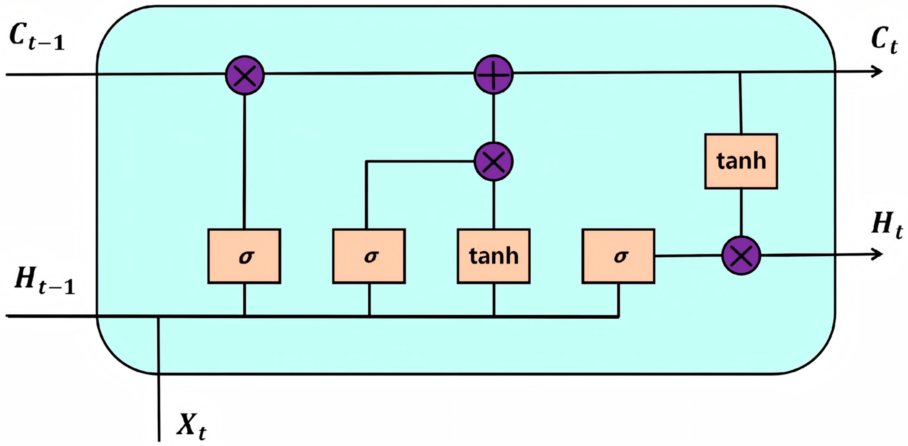
Long Short-Term Memory (LSTM) is a specialized type of Recurrent Neural Network (RNN) designed to address the vanishing or exploding gradient issues encountered by traditional RNNs during the learning of long sequences. By introducing gating mechanisms—including an input gate, a forget gate, and an output gate—the LSTM network is able to capture dependencies better. The input gate filters information to be stored, the forget gate selectively clears data that is no longer relevant, and the output gate controls the content of the current output. The LSTM calculation formula is as follows:

$$f_t = \sigma (W_f·[H_{t-1}, X_t] + b_f)$$

(5)

$$i_t=\sigma (W_i·[H_{t-1},{ X}_t]+{ b}_i)$$

(6)

$$g=\tan \mathrm{h} (W_g·[H_{t-1},{ X}_t]+b_g)$$

(7)

$$C_t=f \times C_{t-1}+i \times g$$

(8)

$$O_t=\sigma (W_o·[H_{t-1},{ X}_t]+b_o)$$

(9)

$$H_t=O_t \times \tan \mathrm{h} \left(C_t\right)$$

(10)

In the equation, $f_t$, $i_t$, and $O_t$ represent the outputs of the forget gate, input gate, and output gate, respectively; $C_t$ denotes the memory cell; $H_t$ represents the current hidden state; $W$ and $b$ denote the weight matrix and bias vector; $X_t$ represents the current input; $\sigma$ and $\tan \mathrm{h}$ are activation functions, corresponding to the sigmoid and hyperbolic tangent activation functions, respectively. The specific structure is shown in Figure 3.

(4)

Temporal Convolutional Network (TCN) Model

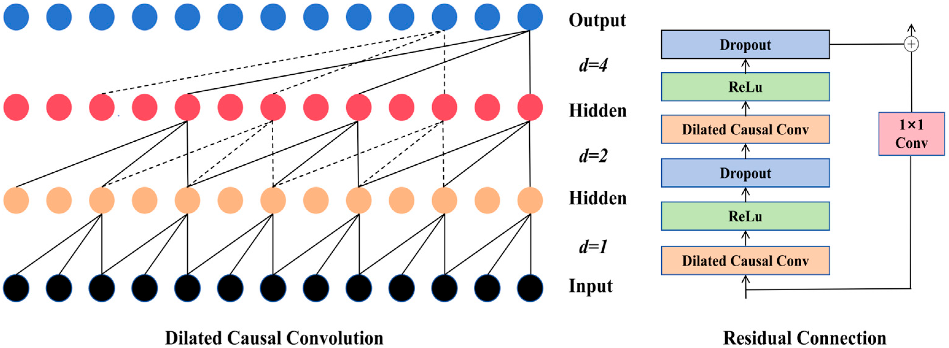
Temporal convolutional networks (TCNs) are a variant of convolutional neural networks (CNNs) specifically designed for sequence modelling. It was first proposed by Lea et al. [30] in 2016. It consists of multiple residual blocks, as shown in Figure 4, where each residual block contains causal convolutions, dilated convolutions, and residual connections. The causal convolutions ensure that the output at time $t$ depends only on the inputs up to and including time t, without relying on future inputs. Specifically, for a causal convolution kernel K = [$K_1,K_2$, …, $K_n$], the output $y_t$ at time t is computed as follows:

$$y_t={\sum }_{i=1}^n{K}_i{X}_{t-i+1}$$

(11)

In the equation, $X_{t-i+1}$ is the input at time $t-i+1$. This approach ensures the model adheres to causal logic when processing time series, avoiding information leakage issues. Dilated convolution allows the convolution kernel to expand its receptive field without increasing the number of parameters, thereby capturing longer-term dependencies in time series. Dilated convolution is achieved by inserting gaps between kernel elements. The dilated convolution output $y_t$ at time t is:

$$y_t={\sum }_{i=1}^k{K}_i{X}_{t-(i-1) \mathrm{d}}$$

(12)

In the equation, $d$ is the dilation factor, and $k$ is the kernel size. As the dilation factor increases, the receptive field expands accordingly.

(5)

TCN-Attention Model (TA)

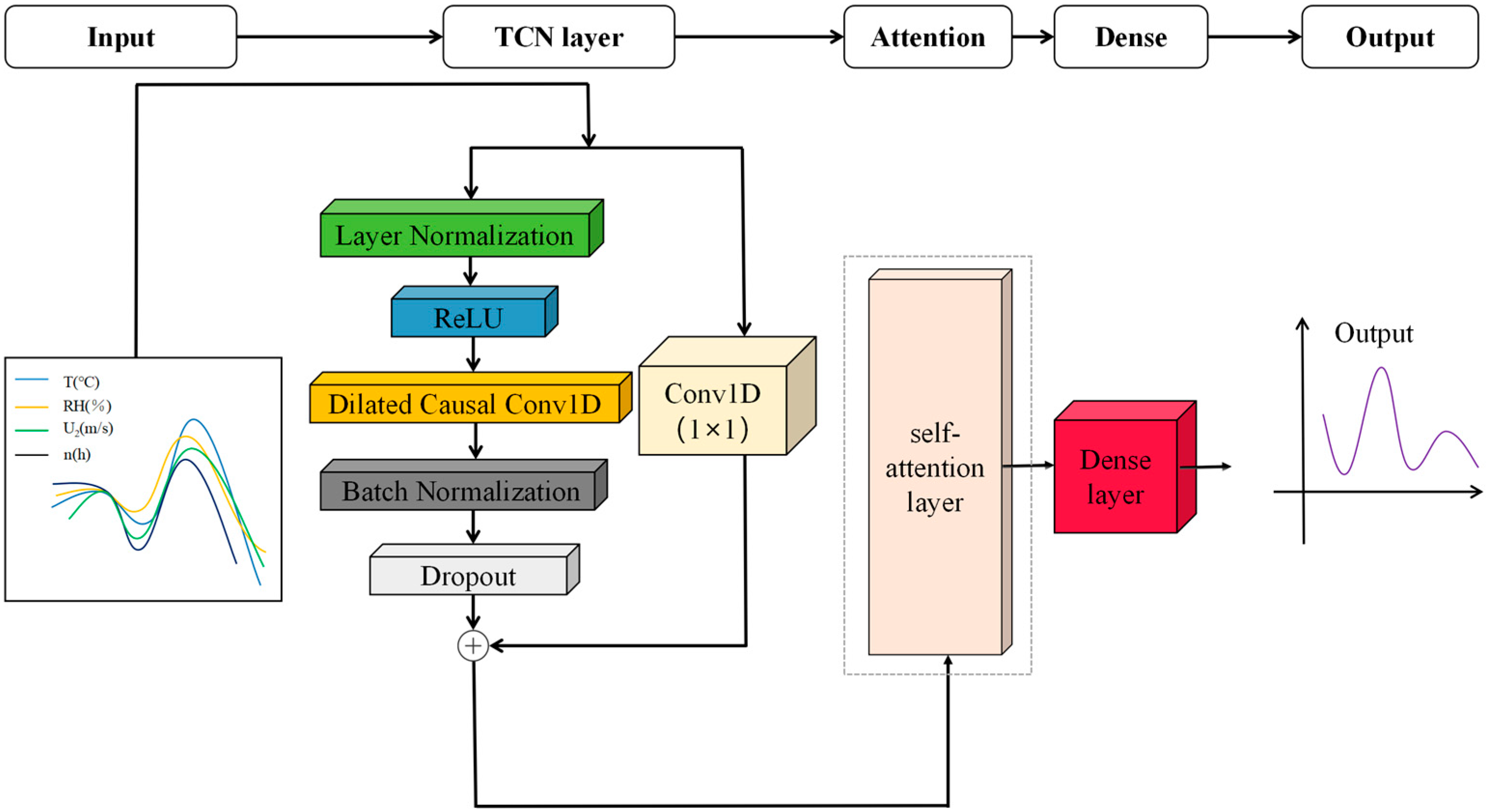
This model utilizes TCN for crop latent evapotranspiration prediction, and a self-attention mechanism [31] is introduced to enhance its performance further. The architecture of the TA model is shown in Figure 5. TCN employs causal dilated Conv1D to extract information from time series data. This dilated Conv1D expands the receptive field by skipping values at fixed intervals in the input data while preserving causality, applying filters over regions larger than their own length. This enables the network to achieve a large receptive field with fewer layers. Residual connections link inputs to outputs from a set of previous layers. The convolutional block design ensures critical features are effectively propagated to the network’s final layers, helping mitigate the vanishing gradient problem in deep networks. To prevent overfitting, the study employs normalization layers and dropout techniques.

The self-attention mechanism utilizes a query-key-value (QKV) model, where Q, K, and V are derived from the same input data. Different linear transformations applied to the input matrix yield the query matrix Q, key matrix K, and value matrix V. Next, the product of Q and the transpose of K is computed to obtain the correlation matrix A. Applying the Softmax function to A yields the normalized correlation matrix A’. Finally, multiplying A′ by V produces the output of the self-attention layer, reflecting the weighted relationships among different elements in the input. Through this mechanism, the model focuses more on important information within the input, enabling more precise and efficient feature extraction. This enhances the model’s ability to capture local features and understand global dependencies. The computation of the self-attention mechanism is as follows.

Calculating the correlation matrix A:

$$\mathrm{A}={\displaystyle \frac{\mathrm{Q}{\mathrm{K}}^{\mathrm{T}}}{\sqrt{{\mathrm{d}}_{\mathrm{k}}}}}$$

(13)

In the equation $Q=X{W}^Q,K=X{W}^K,V=X{W}^V$, $X$ represents the input sequence.

Calculating the output of the self-attention layer:

$$Output = Softmax(A) V$$

(14)

2.3. Data Preprocessing and Visualization

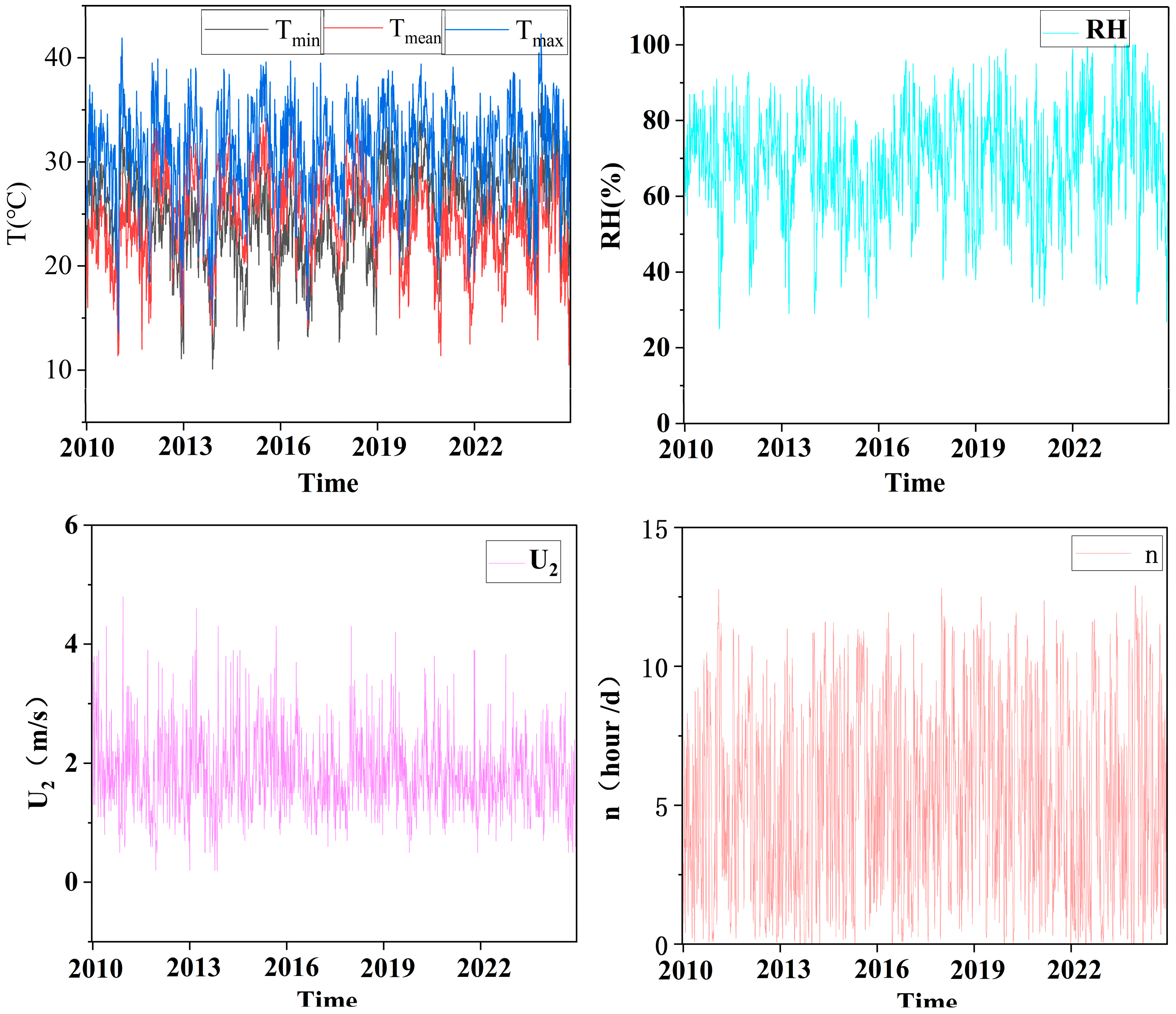
As shown in

Table 1. Meteorological input scenarios for four models.

Scenario	Model			Input	Output
S1	TA	TCN	LSTM	Tmax, Tmean, Tmin	ET0
S2				Tmax, Tmean, Tmin, RH	ET0
S3				Tmax, Tmean, Tmin, n	ET0
S4				Tmax, Tmean, Tmin, U2	ET0

, this study selected four input combination scenarios to evaluate the impact of different meteorological variables on daily ET₀ predictions. Visualization of daily meteorological data for the test site, before data preprocessing, is presented in Figure 6. Temperature and relative humidity are standard observation items at weather stations, while there are fewer stations that can simultaneously observe sunshine hours and wind speed. Therefore, temperature is applied to all input combinations.

Figure 6 shows the temporal variations in the main meteorological parameters during the growth period of summer maize in the study area from 2010 to 2024, including temperature (T), relative humidity (RH), wind speed at 2 m (U₂), and sunshine duration (n). Overall, the meteorological elements display typical seasonal characteristics throughout the growing period, consistent with the climate conditions of northern Henan, which features hot, rainy summers with ample sunshine. During the growth period, the maximum temperature mostly ranges between 30 and 35 °C, and the mean temperature ranges from 25 to 30 °C, both within the suitable temperature range for summer maize growth. Relative humidity fluctuates between 60% and 85%, rising significantly during the rainy summer period, reflecting the synchronized rain and heat typical of the region’s climate. Sunshine duration is generally long, averaging 5–8 h per day, providing sufficient energy for crop photosynthesis and transpiration. Wind speed is overall low, mostly remaining between 1.5 and 2.5 m/s, having a relatively stable effect on evapotranspiration. The dynamic changes in these meteorological factors form an important environmental background that affects ET₀ and provides the data foundation for constructing the ET₀ prediction model in this study.

2.4. Description of the Proposed Model Parameters

The hardware platform in this study utilized an NVIDIA GeForce RTX 4060 GPU with 8 GB of memory(manufacturer: ASUS; location of procurement: Taipei City, Taiwan, China) and was configured with CUDA version 11.3. The model was trained using the Python 3.12.4 programming language and the PyTorch 1.12.0 deep learning framework, with the Adam optimizer employed to optimize training loss. The experiments primarily relied on libraries such as torch, numpy, pandas, and scikit-learn, with specific model parameter configurations detailed in

Table 2. Description of the proposed models and parameters used.

Parameter	TA	TCN	LSTM
num_blocks	4	4	-
hidden_size	32–256	32–256	64
num_layers	-	-	2
epochs	200	200	200
kernel_size	3	3	-
Whether batch normalization is used	Yes	Yes	No
Dropout rate to prevent overfitting	0.2	0.2	-
Learning rate for the optimizer	0.001	0.001	0.001
Optimization algorithm	Adam	Adam	-
Whether self-attention is used	Yes	No	No
Activation function	ReLU	ReLU	-

.

2.5. Evaluation Metrics

This study selects mean absolute error (MAE), mean absolute percentage error (MAPE), root mean square error (RMSE), and coefficient of determination (R²) to evaluate the model’s calculation accuracy. The formulas for each metric are as follows:

$$\mathrm{MAE} = {\displaystyle \frac{1}{\mathrm{m}}}{\sum }_{\mathrm{j}=1}^{\mathrm{m}}\left|Y_j-X_j\right|$$

(15)

$$\mathrm{MAPE}={\displaystyle \frac{1}{\mathrm{m}}}{\sum }_{\mathrm{j}=1}^{\mathrm{m}}\left|{\displaystyle \frac{Y_j-X_j}{X_j}}\right|$$

(16)

$$\mathrm{RMSE} =\sqrt{{\displaystyle \frac{1}{m}}\sum _{j=1}^m{\left(Y_j-X_j\right)}^2}$$

(17)

$${\mathrm{R}}^2={\displaystyle \frac{{\left[\sum _{j=1}^m(X_j-\overline{X})(Y_j-\overline{Y})\right]}^2}{\sum _{j=1}^m{{(X}_j-\overline{X})}^2\sum _{j=1}^m{{(Y}_j-\overline{Y})}^2}}$$

(18)

In the equation,$Y_j$ is the ET₀ calculated by the model on the j-th day; $X_j$ is the standard ET₀ calculated by the P-M model on the j-th day; $\overline{X}$ is the average of $X_j$; $\overline{Y}$ is the average of $Y_j$; m is the sample size; the smaller the MAE, MAPE, and RMSE, the smaller the model’s calculation error; R² closer to 1 signifies higher computational accuracy.

3. Results and Analysis

3.1. Feature Selection

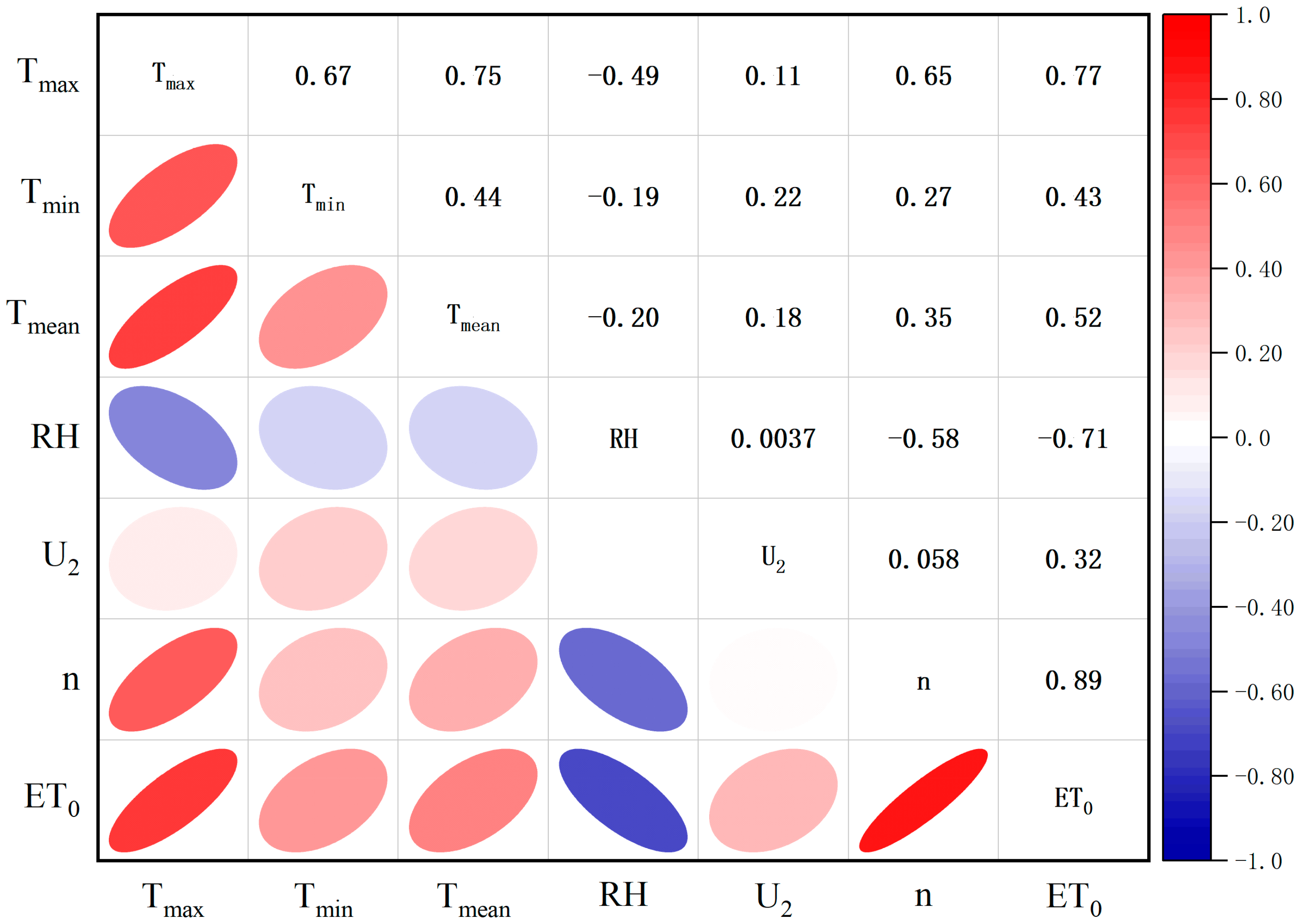
Correlation analysis was used to calculate the coefficient of determination among meteorological factors (Figure 7) to screen factors highly correlated with ET₀. Results indicate that T_max, RH, and n exhibit significant correlations with ET₀ (p < 0.05, R² > 0.71). Among these, RH shows a negative correlation with ET₀, while T_min, T_mean, and U₂ shows moderate correlations with ET₀, with R² ranging from 0.32 to 0.52. To further investigate the importance of meteorological factors and predict evapotranspiration, the maximum information coefficient (MIC) method was used to calculate MIC values between meteorological characteristics and evapotranspiration. The MIC value between sunshine duration and evapotranspiration was 0.857, the highest among all MIC values. Second, the MIC between T_max and evapotranspiration was 0.586. The MICs between T_mean, T_min, RH, U₂, and evapotranspiration were 0.196, 0.176, 0.439, and 0.172, respectively. In summary, the importance of each feature for evapotranspiration follows the order: n > T_max > RH > T_mean > T_min > U₂.

3.2. Overall Accuracy Evaluation of Different Models

Table 3. Statistical results of three prediction models under different input scenarios.

Scenario	Model	MAE	MAPE	RMSE	R2
S1	TA	0.439	10.6%	0.552	0.893
	TCN	0.648	16.1%	0.764	0.855
	LSTM	0.632	15.6%	0.766	0.826
S2	TA	0.204	5.3%	0.257	0.972
	TCN	0.330	8.6%	0.424	0.950
	LSTM	0.491	13.1%	0.558	0.938
S3	TA	0.398	9.8%	0.504	0.921
	TCN	0.482	12.2%	0.587	0.909
	LSTM	0.584	15.0%	0.679	0.885
S4	TA	0.435	10.9%	0.547	0.909
	TCN	0.588	15.3%	0.700	0.871
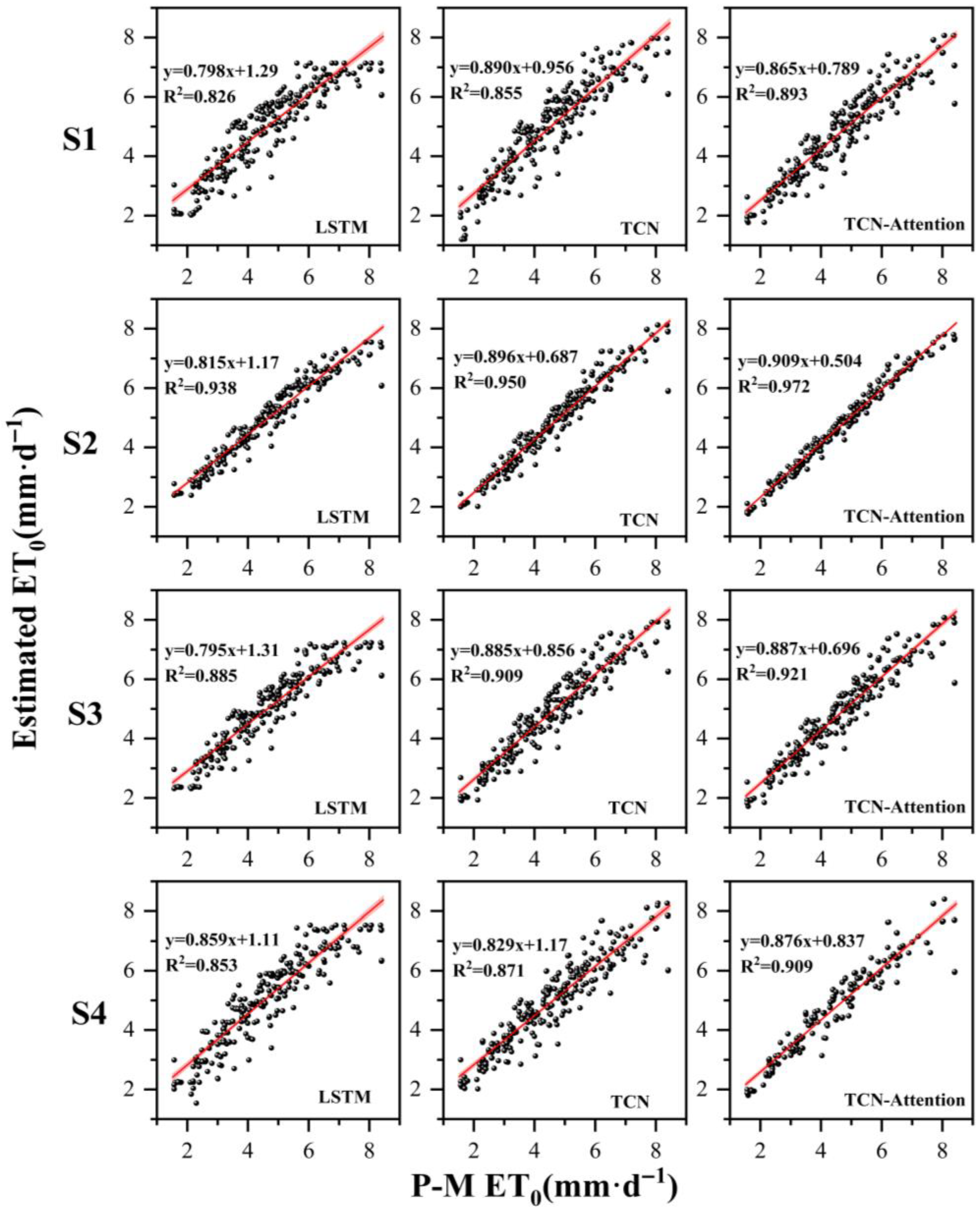
	LSTM	0.662	16.6%	0.769	0.853

shows the model performance results under four limited data input scenarios during the testing period from 2022 to 2024. Under the same input conditions, the TA model performed best in ET₀ estimation. The model’s R² ranged from 0.893 to 0.972, MAE was between 0.204 and 0.439 mm/d, MAPE ranged from 5.3% to 15.3%, and RMSE was between 0.257 and 0.552. Compared with TCN and LSTM models, TA reduced MAE by 17.43% to 58.45%, MAPE by 19.67% to 59.54%, and RMSE by 14.14% to 53.94%, while R² increased by 1.32% to 8.11%, indicating that this model can systematically and accurately estimate ET₀ overall.

For the four model input scenarios S1, S2, S3, and S4, the TA model with input scenario S2 achieved an MAE of 0.204, MAPE of 5.3%, RMSE of 0.257 mm/d, and R² of 0.972, showing better accuracy. Therefore, this study considers the combination of the S2 scenario and the TA model to be the best prediction setup under limited data input conditions.

Figure 8 presents a scatter plot comparing daily ET₀ values calculated by the P-M method against predictions from three models (TA, TCN, and LSTM) during the testing period. The models’ predictions correlate with the P-M calculated values, with most data points clustered near the diagonal line. This indicates that all three models capture the overall trend of ET₀ values, though significant differences emerge across different scenarios. In scenarios S1 and S4, data points exhibit higher dispersion than the fitted line, indicating reduced prediction accuracy under these conditions. Conversely, scenarios S2 and S3 demonstrate a stronger correlation between calculated and predicted values, with the TA model’s data points clustering more closely around the fitted line, reflecting higher predictive precision. Although the TCN and LSTM models also follow the fitted line, their dispersion is slightly higher, resulting in prediction accuracy that is somewhat inferior to that of the TA model. The TA model demonstrates superior predictive performance across all scenarios, exhibiting the smallest deviation between its predictions and the P-M calculated values. This outcome confirms that the TA model can achieve high accuracy in predicting ET₀, even under conditions of limited meteorological data.

3.3. Performance Comparison of Temperature-Based Estimation Models

This study used three deep learning algorithms, including LSTM, TCN, and TA, to construct an ET₀ estimation model based on temperature data. In the empirical formulas based on temperature data, the H-S formula was selected for comparison with the deep learning models.

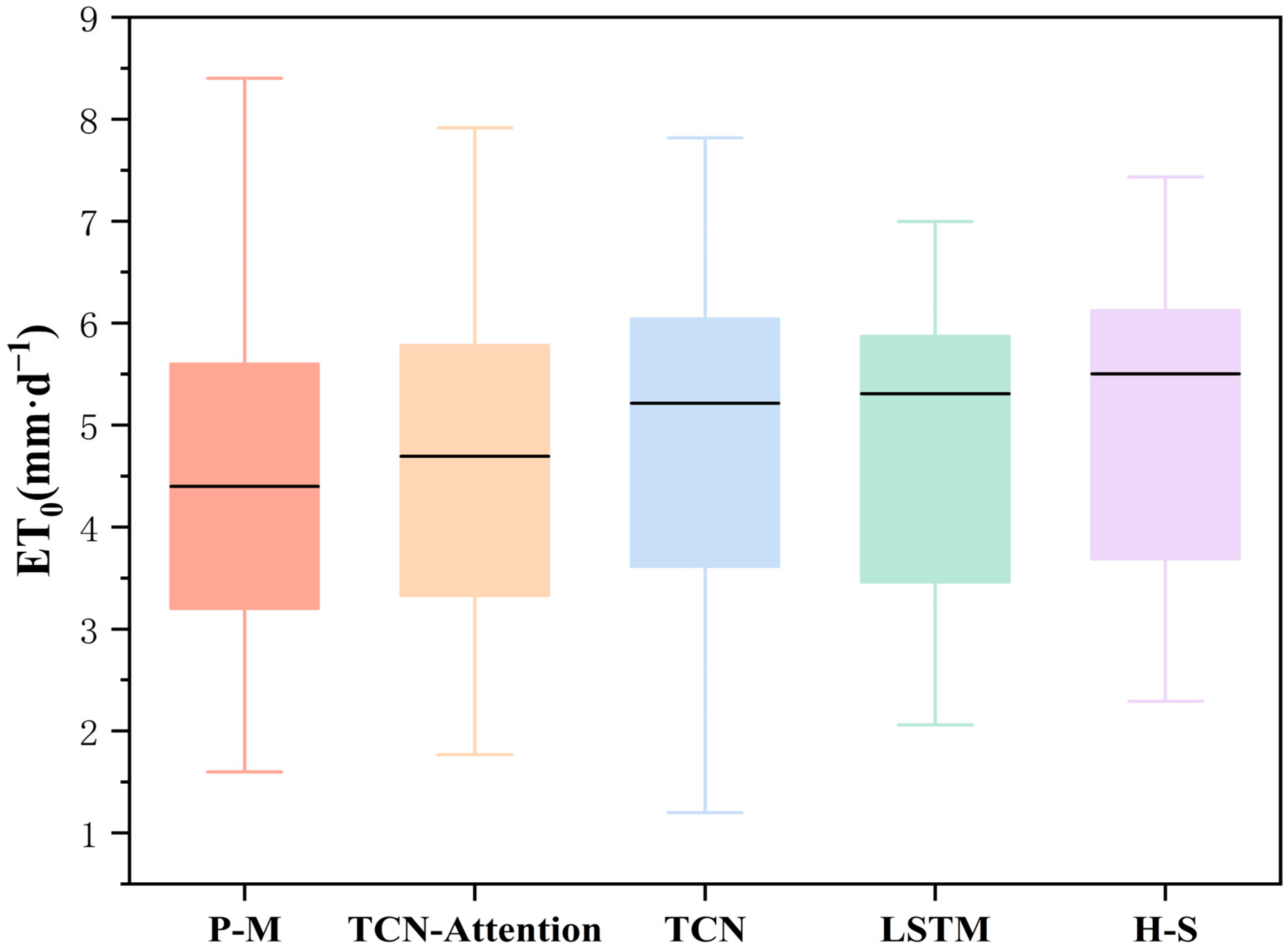
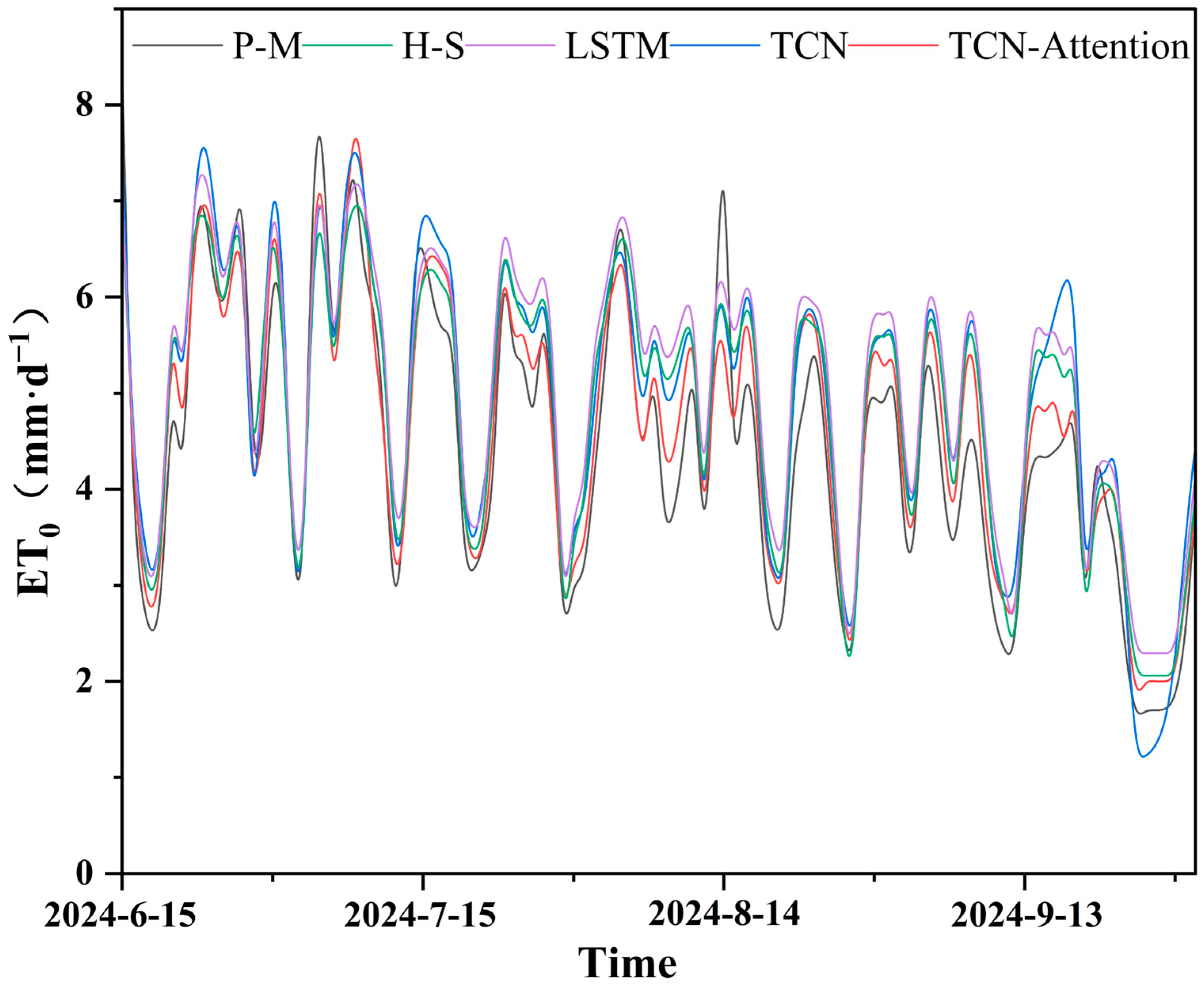
Figure 9 and Figure 10 respectively show the box plots of ET₀ estimates from different models based on the S1 input scenario and the scatter fitting plots of daily ET₀. These visualizations intuitively demonstrate the performance estimation models of data-driven ET₀ and provide a comprehensive comparison between machine learning models and empirical formulas. The results indicate that although the H-S empirical model yields acceptable estimates when meteorological data are lacking, deep learning models, especially TA, offer a more reliable method for calculating ET₀.

Figure 10 presents the time series variations in daily values calculated using the P-M method and the H-S empirical method in the study area under four input scenarios during the test period, as well as the daily values predicted by three models. Overall, all three models are able to reproduce the seasonal variation trends, but there are significant differences in their accuracy in capturing peaks and troughs. Compared with the TCN and LSTM models, under all scenarios, the TA model has lower overestimated and/or underestimated predicted values. Among them, under scenario S2, the TA model performs the best, with the predicted curve very closely fitting the P-M method calculated curve, and the peak error being less than 0.2 mm d⁻¹. In general, the results in Figure 10 reflect that under input conditions of temperature only, the TA model provides the best predictive performance, with prediction accuracy and stability superior to the other two models, further confirming its superiority and reliability in forecasting tasks.

3.4. Model Performance Analysis at Different Time Steps

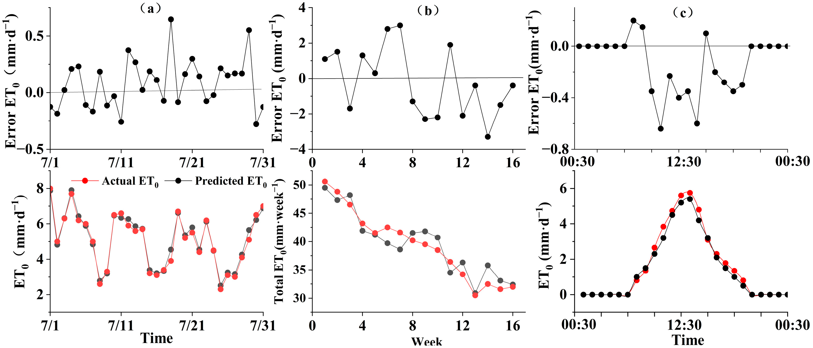
To evaluate the applicability of the TA model combined with the S2 scene at different temporal scales, this study selected daily evapotranspiration data from 1 to 31 July 2024 for analysis at the daily scale. Figure 11a illustrates that the model’s prediction curve closely aligns with actual observations, yielding a coefficient of determination (R²) of 0.975. This indicates exceptionally high prediction accuracy at the daily scale with overall minimal prediction errors. Furthermore, weekly cumulative evapotranspiration data from 15 June to 30 September 2024 were analyzed at the weekly scale. The model successfully captured the growth-stage and seasonal variations in summer maize evapotranspiration, achieving an R² value of 0.928. This demonstrates the model’s ability to accurately predict the overall trend of weekly cumulative evapotranspiration at this scale. Finally, a daily variation analysis of evapotranspiration was conducted using hourly data, selecting 24 hourly datasets from 12 August 2024. The model also performed exceptionally well at high-frequency timescales, achieving an R² value of 0.982. Figure 11c shows that, despite some errors near peak values, prediction errors were generally minor at most time points. The performance comparison of the TA model across the three time steps is summarized in

Table 4. Performance comparison of the TA model across three time steps.

Step Size	MAE/(mm·d−1)	MAPE/(mm·d−1)	RMSE/(mm·d−1)	R2
1 h	0.182	10.2%	0.26	0.982
1 d	0.195	4.52%	0.31	0.975
7 d	0.387	4.65%	2.85	0.928

. In summary, the TA model demonstrated outstanding performance on a daily, weekly, and hourly basis, particularly exhibiting robust applicability and accuracy at high-frequency temporal scales.

4. Discussion

Selecting optimal meteorological inputs and their associated scenarios is crucial for improving the accuracy of model predictions for ET₀. This study utilized correlation analysis and the maximum information coefficient (MIC) method to screen meteorological factors and identify the most critical input parameters for predicting ET₀. Results indicate that sunshine duration is the primary sensitive factor influencing ET₀ in northern Henan Province, which is consistent with findings by Wang Peng Tao et al. [32] on reference crop evapotranspiration in the North China Plain. It also aligns with Feng Zhuangzhuang’s conclusion regarding the significant impact of sunshine duration on ET₀ [33]. The following most influential factors were maximum temperature (T_max) and relative humidity ($\mathrm{R}\mathrm{H}$), consistent with Yang Jialin [34], finding that summer ET₀ on the North China Plain is most sensitive to sunshine duration and temperature. These findings also resonate with the research by LIU [35] and Pan et al. [36], who indicated that variations in ET₀ are primarily influenced by sunshine duration, relative humidity, and temperature. Selecting T and RH as meteorological variables achieves prediction accuracy that is suitable for practical applications. These variables can serve as input parameters for forecasting ET₀ in northern Henan in scenarios with missing meteorological data.

This study also compared the prediction accuracy of LSTM, TCN, and TA models with the H-S empirical model when only temperature data was input. Results indicate that all three models can reproduce the seasonal variation trends of ET₀, though their precision in capturing peak and trough values differs significantly. Compared to the LSTM model, the TA model better avoids gradient vanishing or exploding issues when handling long-sequence data. Furthermore, the attention mechanism in the TA model effectively filters feature vectors that have a greater influence on evapotranspiration, demonstrating stronger nonlinear fitting capabilities. This addresses the significant prediction errors observed in the TCN model when forecasting partial peaks in daily ET₀, which is consistent with the findings by Lin et al. [37] Building upon this research, this study further analyzes the model’s applicability across different temporal scales, revealing peak accuracy at the hourly scale—consistent with Zhao XiuYan et al.’s findings [38] on tea garden evapotranspiration prediction models.

This study, based on data from the Zhengzhou Meteorological Station, constructs a TA model to achieve high-precision predictions of ET₀ for the next 1–7 days. Compared to traditional empirical formulas, this method can more accurately reflect the variation characteristics of ET₀, providing a reliable basis for regional evapotranspiration calculations. Farmers and irrigation management departments can use ET₀ forecasts for the coming days to calculate crop water requirements and develop dynamic, precise irrigation plans, thereby avoiding over- or under-irrigation associated with traditional fixed schedules. At the same time, optimizing water supply helps stabilize and increase the yield of major crops such as summer maize, which is of positive significance for ensuring regional food security and water safety.

It should be particularly noted that this study’s model was trained and validated using data from a single site. Zhengzhou is located in the core area of northern Henan and has a warm temperate continental monsoon climate, which is fairly typical and representative of the region. Existing studies also indicate that the climate conditions in the northern Henan Plain are relatively uniform. Therefore, this model can provide valuable reference for ET₀ predictions in the northern Henan area. However, we also acknowledge that there are some microclimatic differences within the northern Henan region, and this study did not consider the impact on ET₀ when key meteorological data during the summer maize growth period exceeded standard thresholds. Future research will collect meteorological data from more stations and explore the effects of meteorological factors, crop factors, soil factors, and other influences, fully considering various field factors to optimize the model and build a more comprehensive ET₀ prediction system.

5. Conclusions

This study innovatively combines the self-attention mechanism with temporal convolutional networks, proposing a TA model for ET₀ prediction that is suitable for limited meteorological data. Using daily meteorological data during the summer maize growing season from 2010 to 2024 in Zhengzhou, northern Henan, and taking the P-M method results as a reference, the study compared the predictive performance of three deep learning models (LSTM, TCN, and TA) under four limited input scenarios. The results indicate that the TA model performed the best, with prediction accuracy significantly superior to the other models. In the scenario where only temperature data was input, this model outperformed the traditional H-S empirical method. When both temperature and humidity data were input, the model achieved R² values above 0.92 across different prediction horizons, demonstrating good stability and reliability. Therefore, the TA model can serve as an effective tool for estimating ET₀ in the northern Henan region under conditions of missing meteorological data, providing technical support for regional water-saving irrigation and water resource management.

Although the entire article mentions that the proposed models exhibit high accuracy, their limitations cannot be ignored. The models’ adaptability to different regions and effectiveness under complex field conditions still need further validation. Future work will focus on two main aspects: on one hand, collecting meteorological observation data from multiple stations across regions to enhance the models’ generalization ability through cross-station training and testing; on the other hand, integrating crop coefficients, soil types, and other factors into the ET₀ prediction framework to build a more targeted crop water requirement estimation system from the perspective of crop physiological mechanisms. Given the severe agricultural water shortage and limited annual rainfall in northern Henan, the results of this study are crucial for optimizing irrigation systems and formulating regional water resource management strategies.

References

1. Deng, Q.; Sharretts, T.; Ali, T.; Ao, Y.Z.; Chiarelli, D.D.; Demeke, B.; Marston, L.; Mehta, P.; Mekonnen, M.; Rulli, M.C.; et al. Deepening Water Scarcity in Breadbasket Nations. Nat. Commun. 2025, 16, 1110. [Google Scholar] [CrossRef] [PubMed]
2. Tabari, H.; Kisi, O.; Ezani, A.; Hosseinzadeh Talaee, P. SVM, ANFIS, Regression and Climate Based Models for Reference Evapotranspiration Modeling Using Limited Climatic Data in a Semi-Arid Highland Environment. J. Hydrol. 2012, 444–445, 78–89. [Google Scholar] [CrossRef]
3. Liu, Z.; Gao, M.; Liu, F.; Wei, S.; Zhang, H.; Yuan, H.; Li, Q.; Zong, R. Evapotranspiration Partitioning and Crop Water Productivity under Varying Planting Densities of Maize in North China. Crop J. 2025, 13, 952–960. [Google Scholar] [CrossRef]
4. Baratto, P.F.B.; Cecílio, R.A.; De Sousa Teixeira, D.B.; Zanetti, S.S.; Xavier, A.C. Random Forest for Spatialization of Daily Evapotranspiration (ET0) in Watersheds in the Atlantic Forest. Environ. Monit. Assess 2022, 194, 449. [Google Scholar] [CrossRef] [PubMed]
5. Yonaba, R.; Tazen, F.; Cissé, M.; Mounirou, L.A.; Belemtougri, A.; Ouedraogo, V.A.; Koïta, M.; Niang, D.; Karambiri, H.; Yacouba, H. Trends, Sensitivity and Estimation of Daily Reference Evapotranspiration ET0 Using Limited Climate Data: Regional Focus on Burkina Faso in the West African Sahel. Theor. Appl. Climatol. 2023, 153, 947–974. [Google Scholar] [CrossRef]
6. Rajput, J.; Singh, M.; Lal, K.; Khanna, M.; Sarangi, A.; Mukherjee, J.; Singh, S. Performance Evaluation of Soft Computing Techniques for Forecasting Daily Reference Evapotranspiration. J. Water Clim. Change 2023, 14, 350–368. [Google Scholar] [CrossRef]
7. Tan, Q.; Liu, Y.; Pan, T.; Song, X.; Li, X. Changes and Determining Factors of Crop Evapotranspiration Derived from Satellite-Based Dual Crop Coefficients in North China Plain. Crop J. 2022, 10, 1496–1506. [Google Scholar] [CrossRef]
8. Ghorbani, H.; Kashki, A.; Akbari Azirani, T. Evaluation of Temporal Spatial Changes of Reference Evapotranspiration under the Influence of Climate Change in Gorganroud Watershed in Northern Iran. Model. Earth Syst. Environ. 2024, 10, 6821–6838. [Google Scholar] [CrossRef]
9. Ge, J.; Kang, X.; Bai, Y.; Zhang, X.; Dong, C.; Wang, J. LSTM Applicability of LSTM Model for Calculating Reference Crop Evapotranspiration in the Jialing River Basin. China Rural. Water Hydropower 2024, 11, 62–70. [Google Scholar] [CrossRef]
10. Dong, J.; Zhu, Y.; Jia, X.; Shao, M.; Han, X.; Qiao, J.; Bai, C.; Tang, X. Nation-Scale Reference Evapotranspiration Estimation by Using Deep Learning and Classical Machine Learning Models in China. J. Hydrol. 2022, 604, 127207. [Google Scholar] [CrossRef]
11. Comparative Assessment of Empirical and Hybrid Machine Learning Models for Estimating Daily Reference Evapotranspiration in Sub-Humid and Semi-Arid Climates|Scientific Reports. Available online: https://www.nature.com/articles/s41598-024-83859-6 (accessed on 15 September 2025).
12. Rajput, J.; Singh, M.; Lal, K.; Khanna, M.; Sarangi, A.; Mukherjee, J.; Singh, S. Data-Driven Reference Evapotranspiration (ET0) Estimation: A Comparative Study of Regression and Machine Learning Techniques. Environ. Dev. Sustain. 2023, 26, 12679–12706. [Google Scholar] [CrossRef]
13. Bashir, R.N.; Mzoughi, O.; Shahid, M.A.; Alturki, N.; Saidani, O. Principal Component Analysis (PCA) and Feature Importance-Based Dimension Reduction for Reference Evapotranspiration (ET0) Predictions of Taif, Saudi Arabia. Comput. Electron. Agric. 2024, 222, 109036. [Google Scholar] [CrossRef]
14. Zhu, C.; Qin, A. Forecasting of Reference Crop Evapotranspiration in Huang-Huai-Hai Plain Based on XGBoost Machine Learning Model and Numerical Weather Prediction Data. Chin. Agric. Sci. Bull. 2024, 40, 126–133. [Google Scholar] [CrossRef]
15. Guan, Z.; Qin, C.; Qu, J.; CHE, W. Estimation of reference crop evapotranspiration in the Weihe River basin based on the VMD-BO-SVM framework. South-North Water Transf. Water Sci. Technol. 2025, 23, 526–533. [Google Scholar] [CrossRef]
16. Cao, R.; QIN, A. Hybrid time series and machine learning approach for predicting reference evapotranspiration in North Henan Province. J. Irrig. Drain. 2025, 44, 45–52. [Google Scholar] [CrossRef]
17. Pan, Z.; Liu, Z.; Shen, X.; Zhang, Z.; Shi, K.; Zhang, S. Prediction Model of Reference Crop Evapotranspiration Based on Deep Learning. J. Shanxi Agric. Sci. 2023, 51, 942–952. [Google Scholar] [CrossRef]
18. Xie, J.; Gao, P.; Sun, D.; Chen, W.; Chen, S.; Wang, W. Modeling on Prediction of Evapotranspiration of Citrus Orchard Based on LSTM. Trans. Chin. Soc. Agric. Mach. 2020, 51, 351–356. [Google Scholar]
19. Li, M.; Zhou, Q.; Han, X.; Lv, P. Prediction of Reference Crop Evapotranspiration Based on Improved Convolutional Neural Network (CNN) and Long Short-Term Memory Network (LSTM) Models in Northeast China. J. Hydrol. 2024, 645, 132223. [Google Scholar] [CrossRef]
20. Yin, J.; Deng, Z.; Ines, A.V.M.; Wu, J.; Rasu, E. Forecast of Short-Term Daily Reference Evapotranspiration under Limited Meteorological Variables Using a Hybrid Bi-Directional Long Short-Term Memory Model (Bi-LSTM). Agric. Water Manag. 2020, 242, 106386. [Google Scholar] [CrossRef]
21. Salahudin, H.; Shoaib, M.; Albano, R.; Inam Baig, M.A.; Hammad, M.; Raza, A.; Akhtar, A.; Ali, M.U. Using Ensembles of Machine Learning Techniques to Predict Reference Evapotranspiration (ET0) Using Limited Meteorological Data. Hydrology 2023, 10, 169. [Google Scholar] [CrossRef]
22. Bai, S.; Kolter, J.Z.; Koltun, V. An Empirical Evaluation of Generic Convolutional and Recurrent Networks for Sequence Modeling. arXiv 2018, arXiv:1803.01271. [Google Scholar] [CrossRef]
23. Chen, Z.; Sun, S.; Wang, Y.; Wang, Q.; Zhang, X. Temporal Convolution-Network-Based Models for Modeling Maize Evapotranspiration under Mulched Drip Irrigation. Comput. Electron. Agric. 2020, 169, 105206. [Google Scholar] [CrossRef]
24. Gao, Z.; Zhang, X.; Gao, Z.; Zhou, B.; Liu, Y.; Liu, D.; Ma, X. An Interpretable Hybrid TCN-BiLSTM Model for Reference Evapotranspiration Prediction. Water Resour. Manag. 2025, 39, 1–23. [Google Scholar] [CrossRef]
25. Ren, C.; Wang, Z.; Ma, Z.; Zhang, M. Estimation of Reference Crop Evapotranspiration in Shandong Province Based on Deep Learning and Traditional Machine Learning Model. Water Sav. Irrig. 2022, 03, 67–74. [Google Scholar] [CrossRef]
26. Dong, J.; Xing, L.; Cui, N.; Zhao, L.; Guo, L.; Wang, Z.; Du, T.; Tan, M.; Gong, D. Estimating Reference Crop Evapotranspiration Using Improved Convolutional Bidirectional Long Short-Term Memory Network by Multi-Head Attention Mechanism in the Four Climatic Zones of China. Agric. Water Manag. 2024, 292, 108665. [Google Scholar] [CrossRef]
27. Zhang, B.; Wang, S.; Deng, L.; Jia, M.; Xu, J. Ship Motion Attitude Prediction Model Based on IWOA-TCN-Attention. Ocean Eng. 2023, 272, 113911. [Google Scholar] [CrossRef]
28. Reshef, D.N.; Reshef, Y.A.; Finucane, H.K.; Grossman, S.R.; McVean, G.; Turnbaugh, P.J.; Lander, E.S.; Mitzenmacher, M.; Sabeti, P.C. Detecting Novel Associations in Large Data Sets. Science 2011, 334, 1518–1524. [Google Scholar] [CrossRef] [PubMed]
29. Hargreaves, G.H.; Samani, Z.A. Reference crop evapotranspiration from temperature. Appl. Eng. Agric. 1985, 1, 96–99. [Google Scholar] [CrossRef]
30. Lea, C.; Vidal, R.; Reiter, A.; Hager, G.D. Temporal Convolutional Networks: A Unified Approach to Action Segmentation. In Computer Vision—ECCV 2016 Workshops; Hua, G., Jégou, H., Eds.; ECCV 2016. Lecture Notes in Computer Science; Springer: Cham, Switzerland, 2016; Volume 9915. [Google Scholar] [CrossRef]
31. Wang, Y.; Pang, G.; Wang, T.; Cong, X.; Pan, W.; Fu, X.; Wang, X.; Xu, Z. Future Reference Evapotranspiration Trends in Shandong Province, China: Based on SAO-CNN-BiGRU-Attention and CMIP6. Agriculture 2024, 14, 1556. [Google Scholar] [CrossRef]
32. Wang, P.; Yan, J.; Jiang, C.; Liu, X. Spatial and temporal variations of reference crop evapotranspiration and its influencing factors in the North China Plain. Acta Ecol. Sin. 2014, 34, 5589–5599. [Google Scholar] [CrossRef][Green Version]
33. Feng, Z.; Shi, X.; Miao, Q.; Li, J.; Sun, W.; Dai, L. Prediction of reference crop evapotranspiration in Xilinguole grassland based on multivariate time series model. Arid Zone Res. 2021, 38, 1650–1658. [Google Scholar] [CrossRef]
34. Yang, J.; Liu, C.; Qiao, F.; Du, J.; Wang, M. Seasonal Response of Reference Crop Evapotranspiration to Key Climatic Variables in North China Plain. Clim. Environ. Res. 2016, 21, 418–428. [Google Scholar] [CrossRef]
35. Liu, H.; Li, Y.; Josef, T.; Zhang, R.; Huang, G. Quantitative Estimation of Climate Change Effects on Potential Evapotranspiration in Beijing during 1951–2010. J. Geogr. Sci. 2014, 24, 93–112. [Google Scholar] [CrossRef]
36. Pan, J.; Yu, L.; Zhou, B.; Zhao, J. A Daily Reference Crop Evapotranspiration Forecasting Model Based on Improved Informer. Agriculture 2025, 15, 933. [Google Scholar] [CrossRef]
37. Lin, Y.; Koprinska, I.; Rana, M. Temporal Convolutional Attention Neural Networks for Time Series Forecasting. In Proceedings of the 2021 International Joint Conference on Neural Networks (IJCNN); IEEE: New York, NY, USA, 2021; pp. 1–8. [Google Scholar]
38. Zhao, X.; Wang, B.; Du, X.; Wang, W.; Ding, Z.; Zhou, C.; Zhang, K. Evapotranspiration Prediction Model of Tea Garden Based on Temporal Convolutional Network and Transformer. Trans. Chin. Soc. Agric. Mach. 2024, 55, 337–346. [Google Scholar] [CrossRef]
Figure 1. Overview of the study area and meteorological facilities. Note: (a) Geographic location of the study area; (b) cropping patterns and surrounding environment of the study area; and (c) meteorological facilities in the study area.
Agronomy 16 00435 g001
Figure 2. Research flowchart.
Agronomy 16 00435 g002
Figure 3. LSTM model architecture.
Agronomy 16 00435 g003
Figure 4. TCN model architecture.
Agronomy 16 00435 g004
Figure 5. TA model architecture.
Agronomy 16 00435 g005
Figure 6. Meteorological variation diagram of time series from 2010 to 2024.
Agronomy 16 00435 g006
Figure 7. Correlation analysis of different meteorological variables and reference crop evapotranspiration (ET0).
Agronomy 16 00435 g007
Figure 8. Comparison of prediction model performance under different input scenarios.
Agronomy 16 00435 g008
Figure 9. Comparison of model estimation results based on temperature input scenarios.
Agronomy 16 00435 g009
Figure 10. Daily ET0 time series change plot of the estimation model based on the temperature input scenario.
Agronomy 16 00435 g010
Figure 11. Performance analysis of the TA model at three time steps. Note: (a) Performance analysis of the TA model at daily time step.; (b) Performance analysis of the TA model at weekly time step.; and (c) Performance analysis of the TA model at hourly time step.
Agronomy 16 00435 g011