Study on the Mechanism of Urea Arch Breaking in Vibrating Fertiliser Dischargers Based on EDEM

Abstract

Urea discharge can become unstable as interparticle cohesion increases under moisture-affected conditions. This study combined bulk-solid mechanics, discrete element method (DEM) simulations, contact parameter calibration, and bench testing to investigate urea arching and vibration-assisted discharge. Dry-contact parameters for urea particles and a polypropylene (PP) hopper were calibrated using angle-of-repose and sliding tests. The calibrated simulations differed from the physical target values by 1.71% for the angle of repose and 3.98% for the sliding friction angle. In a separate DEM sensitivity analysis, JKR surface energy was prescribed at 0, 0.05, 0.15, and 0.30 J·m⁻² as an effective adhesion parameter rather than as a calibrated moisture state. The maximum EDEM-exported Total Force signal increased from 2.283 N at 0 J·m⁻² to 2.704 N at 0.30 J·m⁻² (18.5%), whereas the mean particle velocity during the common 5–18 s pre-discharge interval decreased from 0.0613 to 0.0397 m·s⁻¹ (35.3%). Two combined excitation settings were evaluated: 29.17 Hz/0.2 mm and 58.33 Hz/1.2 mm. Because frequency and amplitude changed simultaneously, their individual effects could not be isolated. The bench tests yielded mean discharged masses of 566.808, 492.435, and 464.305 g for the 58.33 Hz/1.2 mm, 29.17 Hz/0.2 mm, and non-vibrating conditions, respectively. The 58.33 Hz/1.2 mm setting increased the mean mass discharged during the 30 s collection interval by approximately 22.1% relative to the non-vibrating control. The corresponding between-run coefficients of variation were 3.628%, 3.580%, and 4.303%; these values describe repeatability between replicate runs rather than temporal or spatial discharge uniformity. Overall, increasing prescribed adhesion reduced particle mobility in the DEM simulations, whereas the 58.33 Hz/1.2 mm combined excitation increased discharged mass under the tested conditions. The experiments do not directly demonstrate crystal bridge rupture or isolate an independent frequency effect.

1. Introduction

Reducing chemical fertiliser inputs while improving fertiliser-use efficiency is a key objective of precision agriculture [1]. Accurate fertiliser detection, metering, and distribution are essential for reliable, mechanised precision fertilisation [2,3,4]. However, granular fertiliser discharge can be disrupted by caking, arching, and blockage, motivating the development of vibrating, ordered-discharge, and mechanical arch-breaking devices [5,6,7,8]. Urea is particularly susceptible to these problems because of its hygroscopicity and tendency to form interparticle bonds after moisture absorption [9,10]. A representative macroscopic arching configuration is shown in Figure 1.

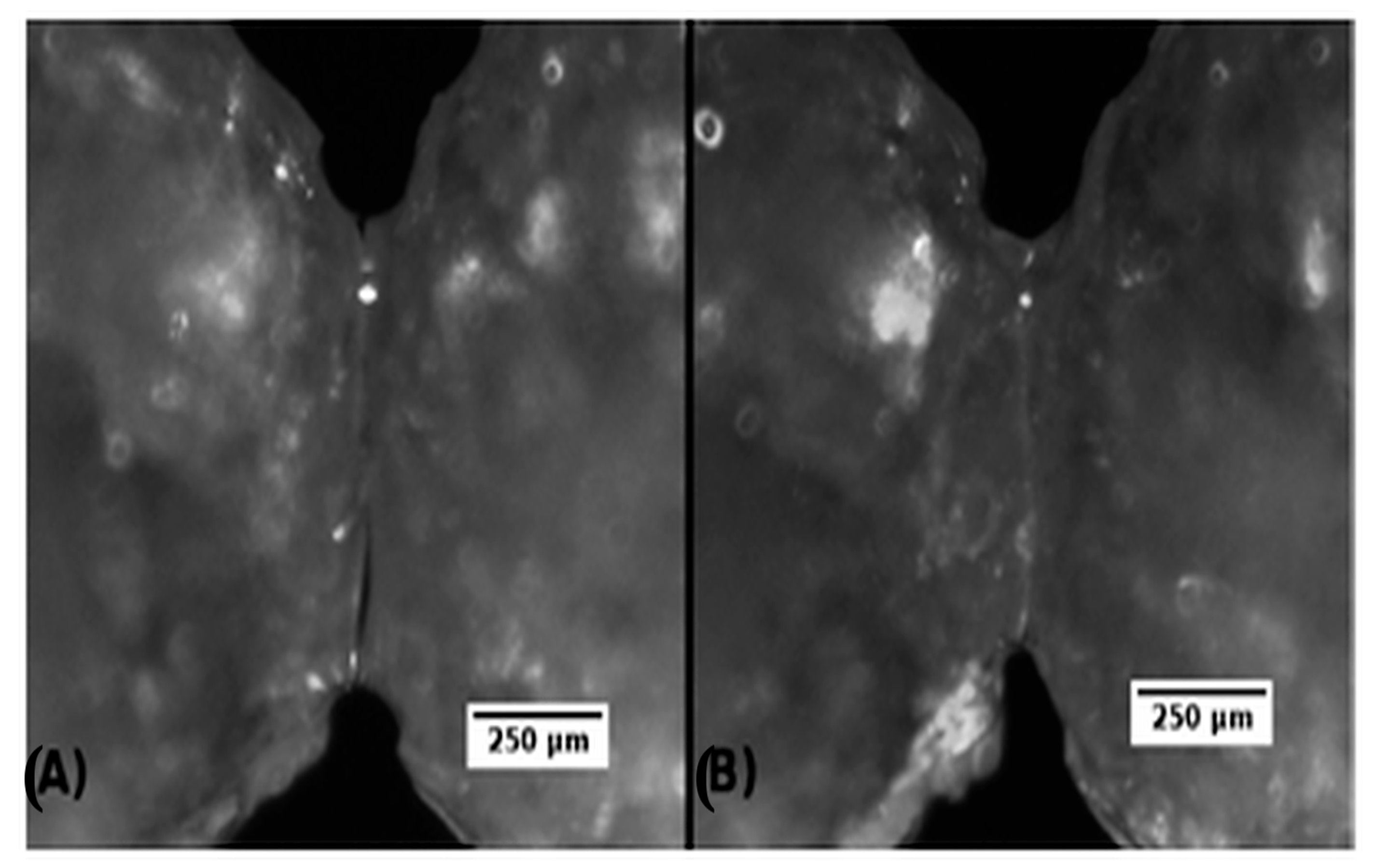
At the microscopic scale, moisture migration, surface dissolution, and subsequent recrystallisation can promote solid bridge formation between urea granules [9,10]. Direct observations of urea prills have documented the development and evolution of such interparticle bridges [10]. These bridges increase the apparent cohesion of the granular bed and strengthen load-bearing contact networks, thereby reducing flowability and facilitating the formation of a self-supporting arch above the discharge outlet. At the macroscopic scale, such arches resist shear deformation and can lead to highly non-uniform flow or complete cessation of discharge. A representative micrograph of intergranular crystal bridges is shown in Figure 2.

Anti-blocking and fertiliser delivery systems include disturbance-cone and centrifugal devices [11,12], blending mechanisms [13], pneumatic variable-rate systems [14,15], and layered seeding/fertilising openers [16]. Linkage- and vibration-assisted approaches have also been investigated [5,8]. These systems can promote particle rearrangement or improve material delivery, but their performance depends on particle properties, hopper geometry, and the imposed mechanical excitation. For cohesive fertilisers, the key issue is not only particle transport but also the stability of load-bearing contact networks near the outlet.

DEM is widely used to calibrate contact parameters and analyse particle–boundary interactions in agricultural particulate systems [17,18,19,20,21]. For granular fertilisers, previous studies have quantified physical and mechanical properties [22,23], calibrated urea contact parameters [24], characterised fertiliser–polymer interactions [25], and evaluated fertiliser-spreader performance [26]. Material properties relevant to DEM parameterisation have also been reported for polypropylene and urea [27,28], while calibration procedures developed for other granular and soil systems provide additional methodological references [29,30]. EDEM–CFD has also been applied to fertiliser-spreader optimisation [31].

Related agricultural DEM studies have investigated particle transport, vibrating feeding and distribution, and soil- or crop-contact mechanisms [32,33,34,35,36,37,38,39,40,41,42]. More generally, particle trajectories, velocities, and energy dissipation in dynamically operated agricultural equipment depend on working-element geometry and operating conditions [43], whereas the transport capacity of rotating elements depends on material motion, rotor kinematics, and system geometry [44]. These studies provide useful modelling and transport-analysis methods, but they do not establish moisture-dependent cohesive contact laws or arch stability criteria for urea discharge.

A key unresolved question is how increasing effective interparticle adhesion alters arching behaviour and how externally imposed vibration modifies discharge. Moisture adsorption, capillary effects, and recrystallisation may increase cohesion in real urea [9,10], whereas a JKR-based DEM model represents only an effective adhesive contact law and does not explicitly simulate moisture uptake, liquid bridge evolution, or crystal growth. The physical moisture mechanisms must therefore be distinguished clearly from the effective adhesion parameter used in the DEM model.

Accordingly, this study uses a Mohr–Coulomb-based limit equilibrium relation as a conceptual description of cohesive arch stability, calibrates dry-contact parameters against physical tests, and then performs a JKR sensitivity analysis using prescribed surface energy levels. Dynamic DEM simulations and bench tests compare two combined vibration settings with a non-vibrating control. The objectives are to (i) quantify how prescribed adhesive contact strength affects simulated particle mobility and retention, (ii) compare discharge responses under the tested combined excitations, and (iii) identify the limitations that must be addressed before attributing the response specifically to moisture-induced crystal bridges or to vibration frequency alone.

2. Materials and Methods

2.1. Conceptual Framework for Cohesive Urea Arching and DEM Representation

Urea is hygroscopic, and exposure to humid environments can promote surface wetting, dissolution, and subsequent recrystallisation, thereby increasing apparent bulk cohesion [9,10]. At the continuum scale, the limiting shear strength of a cohesive granular material can be described by the Mohr–Coulomb criterion:

$${\tau }_f=c+\sigma \tan \phi$$

(1)

where τf is the limiting shear strength (Pa), c is the apparent cohesion (Pa), σ is the normal compressive stress (Pa), and φ is the internal friction angle (°). Here, the Mohr–Coulomb relation is used only as a conceptual framework for discussing how cohesion can influence arch stability. Because c was not independently measured for the urea used in the bench tests, this relation is not used to infer a quantitative moisture-specific arch threshold.

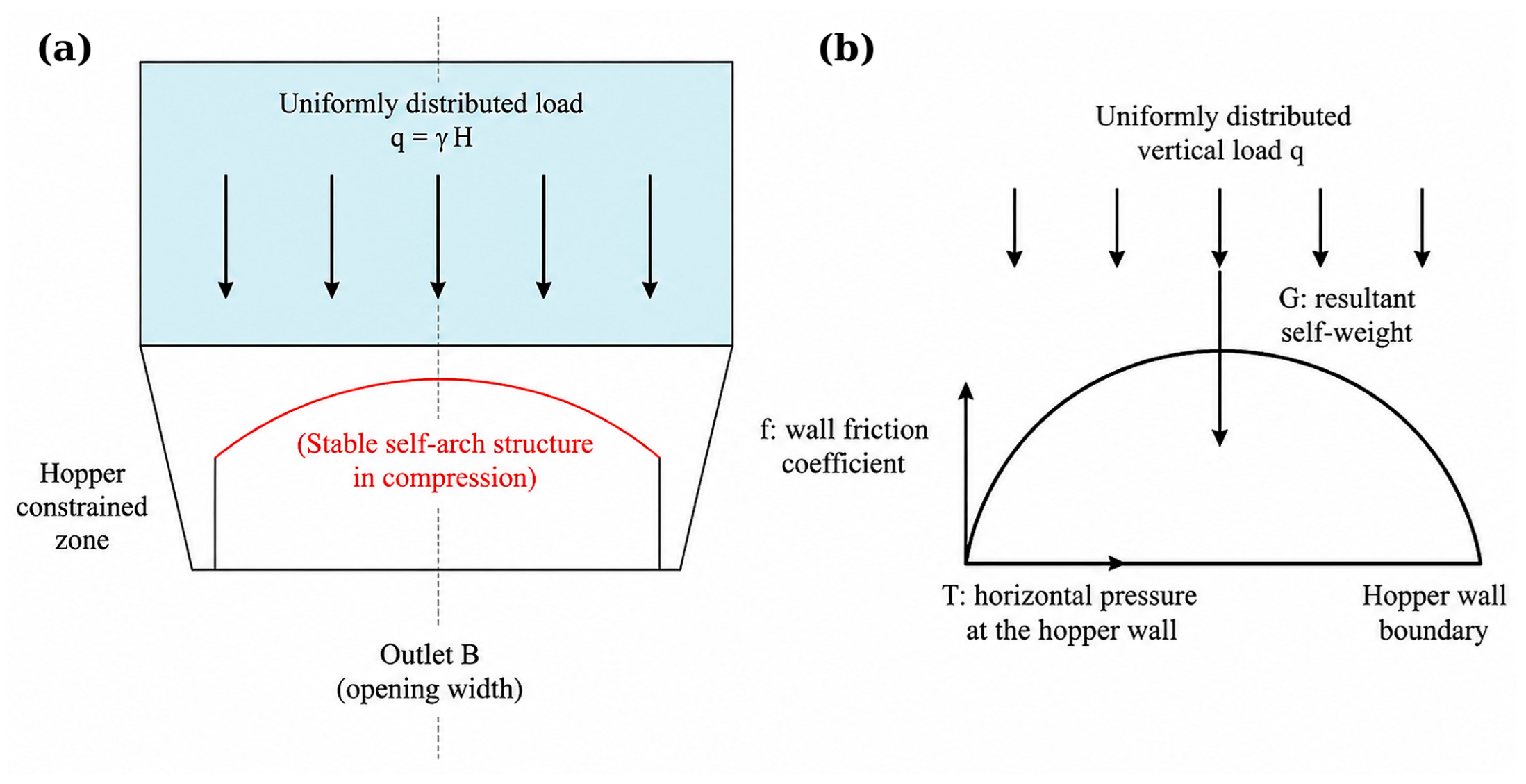
To illustrate how a critical span scales with cohesion, a simplified two-dimensional half-arch free body is considered (Figure 3). For the adopted idealised limit equilibrium relation, the balance at incipient failure is written as c = (γBcr/2) [(1 − sin φ)/sin φ]; rearrangement gives Equation (2). The relation assumes limit equilibrium, uniform unit weight, and a representative internal friction angle. It is used only to illustrate the expected scaling with cohesion and unit weight and is not treated as a quantitatively validated predictor for the present hopper.

$$B_{cr}={\displaystyle \frac{2c}{\gamma }}{\displaystyle \frac{\sin \phi }{1-\sin \phi }}$$

(2)

In Equation (2), γ denotes the bulk unit weight (N·m⁻³), with γ = ρb g, where ρb is the bulk density (kg·m⁻³) and g is gravitational acceleration (9.81 m·s⁻²). For the present hopper, the discharge outlet span is B = 50 mm, and Bcr is the conceptual critical arching span. Because c, φ, and ρb were not independently measured under the bench test conditions, Bcr was not evaluated numerically, and no quantitative comparison between Bcr and B was made.

The standard Hertz–Mindlin contact model represents elastic-frictional contact without an adhesive term. To examine the sensitivity of simulated discharge to added adhesion, the Hertz–Mindlin with JKR contact model was used. In this model, surface energy controls the strength of the adhesive normal contact. Importantly, the JKR model does not simulate moisture adsorption, capillary-liquid evolution, or urea recrystallisation. The surface energy values are therefore treated as prescribed effective adhesion levels rather than as calibrated moisture contents or relative humidity states.

2.2. Selection of Calibration Parameters and Conceptual Micro–Macro Relations

The DEM parameters were grouped into intrinsic material properties and contact parameters [21]. Intrinsic properties were obtained from physical measurements or the literature, whereas contact parameters describe urea–urea and urea–boundary interactions. Because contact behaviour depends on surface morphology and material properties, the contact coefficients were calibrated using physical tests together with DEM simulations.

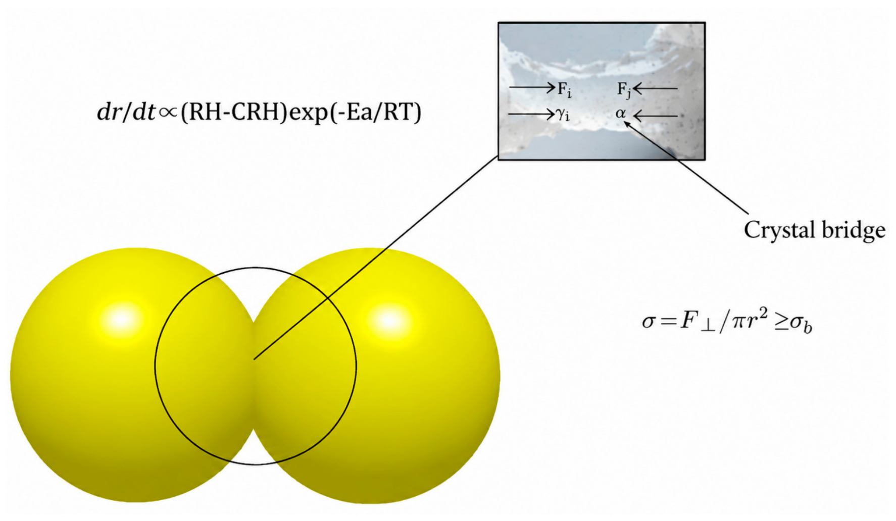
Moisture-related bridge formation can depend on humidity, temperature, and exposure time. Equation (3) is presented only as a conceptual kinetic relation, where r is a characteristic bridge radius, RH is relative humidity, CRH is a critical relative humidity parameter, Ea is an activation energy term, R is the universal gas constant, and T is absolute temperature. This bridge-growth relation was not implemented in EDEM and was not used to assign the JKR surface energies in the simulations.

$${\displaystyle \frac{dr}{dt}}\propto \left(RH-CRH\right)\cdot \exp \left(-{\displaystyle \frac{E_a}{RT}}\right)$$

(3)

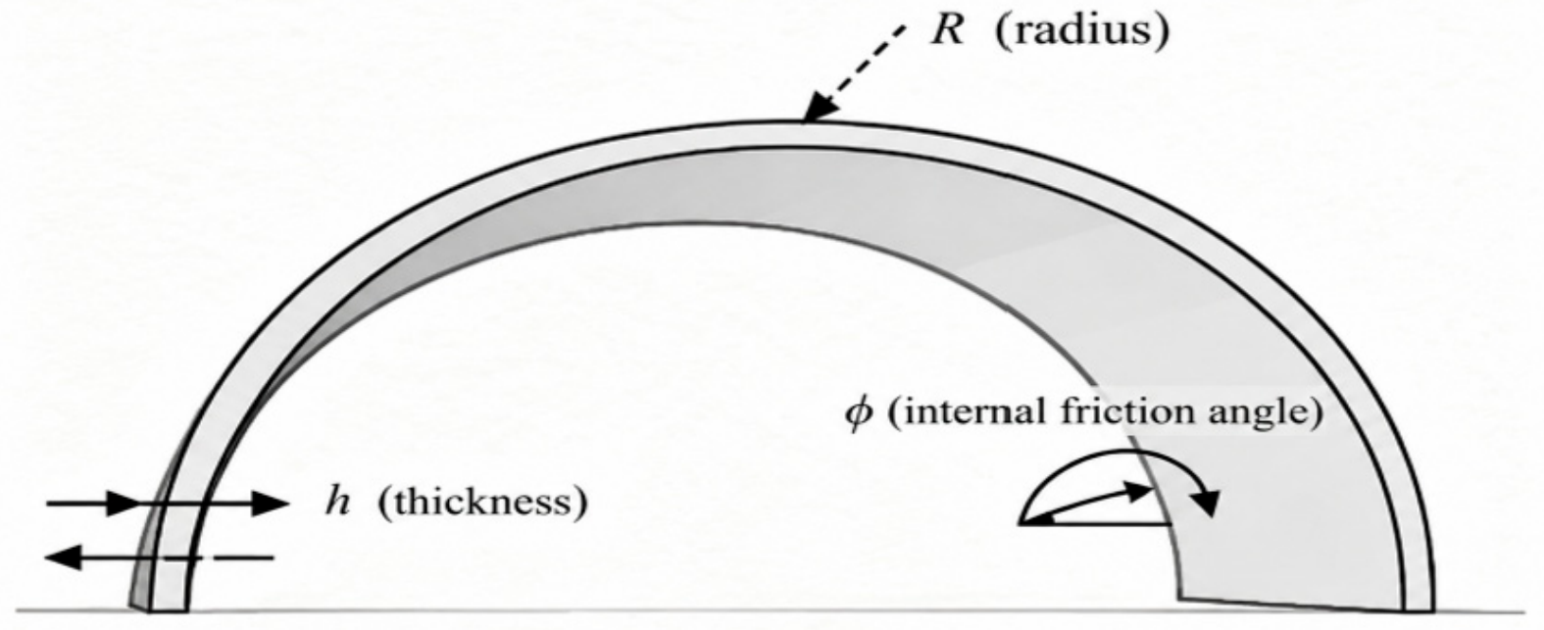
Equation (4) is presented as a schematic stress relation for an idealised arch foot, where σmax is the maximum tensile stress, γ is the bulk unit weight (N·m⁻³), R is the representative arch radius, h is the representative arch thickness, and φ is the internal friction angle. Equation (4) was not used as a bridge fracture criterion in the DEM model; Figure 4 and Figure 5 therefore serve only as conceptual illustrations of the micro–macro framework.

$${\sigma }_{max}={\displaystyle \frac{\gamma R^2}{2h\left(1-\sin \phi \right)}}$$

(4)

The calibrated coefficients of restitution, rolling friction, and static friction define the non-adhesive baseline by controlling collision dissipation and frictional resistance. The subsequent JKR surface energy sweep introduces an additional adhesive contribution. Because surface energy was not mapped to moisture content or crystal bridge geometry, the DEM results quantify sensitivity to prescribed adhesion but do not identify or model the fracture of recrystallised bridges.

Published values [22,23,24,25] were used to define the initial search ranges for urea–urea contact parameters. Direct urea–PP data were not available; therefore, published fertiliser–PVC data [25] were used only to establish initial bounds because PVC and PP are both polymeric boundary materials. The final urea–PP coefficients were not adopted from PVC data; instead, they were calibrated against the physical sliding test performed on the PP plate used in this study.

For physical characterisation, damaged, agglomerated, or visibly irregular urea granules were excluded, and the remaining material was stored in a dry, sealed container before measurement. Particle diameter was measured with a 0–150 mm vernier calliper with 0.01 mm resolution. Three groups of 100 granules were randomly prepared; the laboratory record contains 30 valid diameter measurements per group (n = 90), giving a mean diameter of 1.504 ± 0.057 mm (mean ± SD; range 1.37–1.63 mm). Particle density was measured gravimetrically in five fixed-volume replicates using a 50 cm³ volume and a 0.01 g balance. The measured densities were 1.233, 1.239, 1.230, 1.242, and 1.236 g·cm⁻³, corresponding to 1236 ± 4.7 kg·m⁻³ (mean ± SD). In the DEM model, urea granules were represented as spherical particles with a fixed physical radius of 0.8475 mm (diameter 1.695 mm) and a particle density of 1236 kg·m⁻³. Particle density is distinct from the bulk density ρb used in the continuum arch relation. The single-size spherical representation is a modelling simplification and does not reproduce the measured particle-size and shape distribution. The material properties used in the DEM model are summarised in

Table 1. Material properties used in the DEM model for urea particles and the polypropylene (PP) hopper.

Parameter	Urea	PP Hopper
Poisson’s ratio	0.4	0.45
Shear modulus/Pa	2.8 × 107	7 × 108
Density/kg·m−3	1236	910
DEM particle physical radius/mm	0.8475	—

.

2.3. Calibration Tests and Experimental Design for Contact Parameters

A constrained central composite response surface design was used to calibrate six contact parameters (X₁–X₆): the coefficients of restitution, rolling friction, and static friction for urea–urea contacts and the corresponding coefficients for urea–PP contacts. The urea–urea angle of repose (Y₁) and urea–PP sliding friction angle (Y₂) were used as response variables.

The nominal axial coding coefficient was 1.682. Axial settings that would have produced non-physical negative friction coefficients were constrained to a minimum physical value of 0.01. Consequently, the implemented design is a constrained central composite response surface design rather than a strictly rotatable CCD, and interpretation is limited to the actual factor settings listed in

Table 2. Coded factor levels used in the constrained response surface calibration.

Test	Code Value	Coefficient of Restitution	Coefficient of Rolling Friction	Coefficient of Static Friction
Urea particle packing test	−1.682	0.01	0.01	0.08
	−1	0.05	0.11	0.27
	0	0.26	0.39	0.54
	1	0.47	0.66	0.80
	1.682	0.61	0.84	0.99
Urea particle sliding test	−1.682	0.05	0.01	0.25
	−1	0.15	0.05	0.35
	0	0.30	0.15	0.50
	1	0.45	0.25	0.65
	1.682	0.55	0.32	0.75

Note: The lower bound of 0.01 was imposed to avoid non-physical negative contact coefficients. Consequently, the implemented design is a constrained response surface design rather than an ideal rotatable CCD; the actual settings in Table 2 define the tested design space. Table columns are presented in standard left-to-right order for readability.

.

2.3.1. Urea Accumulation Test (Calibration of the Angle of Repose)

Dry-contact calibration simulations were performed using the standard Hertz–Mindlin model. Because the physical calibration tests were intended to establish the non-adhesive baseline, JKR adhesion was not applied at this stage. A JKR surface energy value of 0 J·m⁻² represents the same non-adhesive limit used as the reference condition in the subsequent sensitivity analysis.

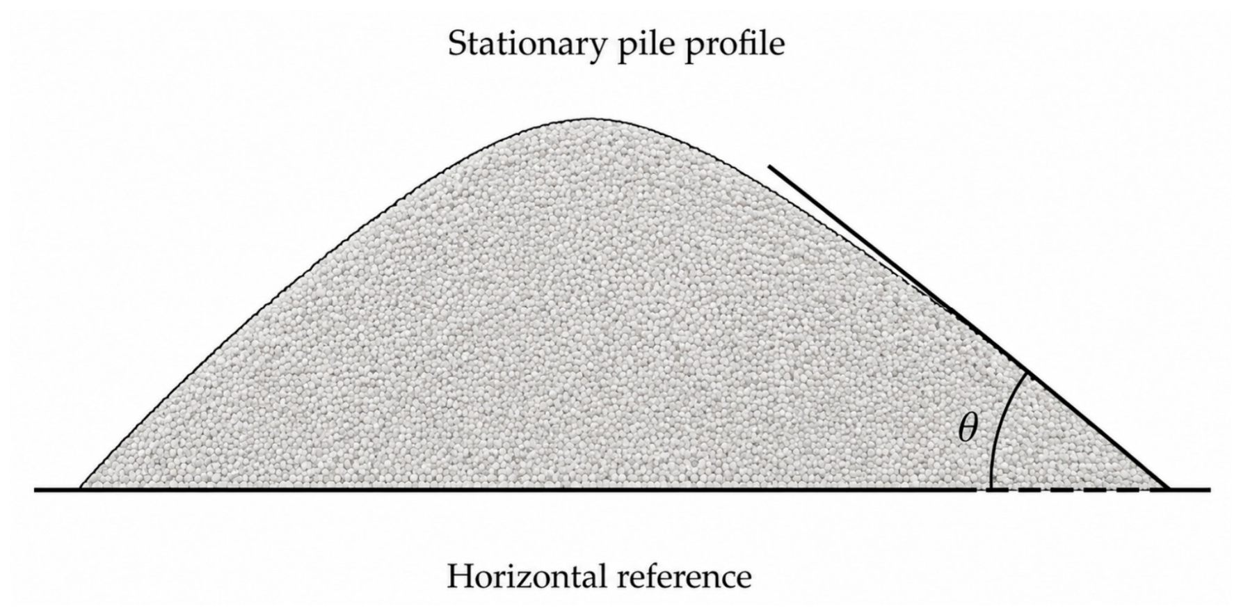
For the angle-of-repose simulation, 1000 spherical particles were generated in EDEM and allowed to fall freely until the pile became stationary. The particles used the fixed spherical geometry described above (physical radius 0.8475 mm). The pile profile was then exported for repose angle measurement. Figure 6 illustrates the angle-of-repose measurement geometry applied to the stationary simulated pile. No formal velocity threshold was defined for stationarity; pile stability was judged from the stationary configuration used for image-based angle measurement.

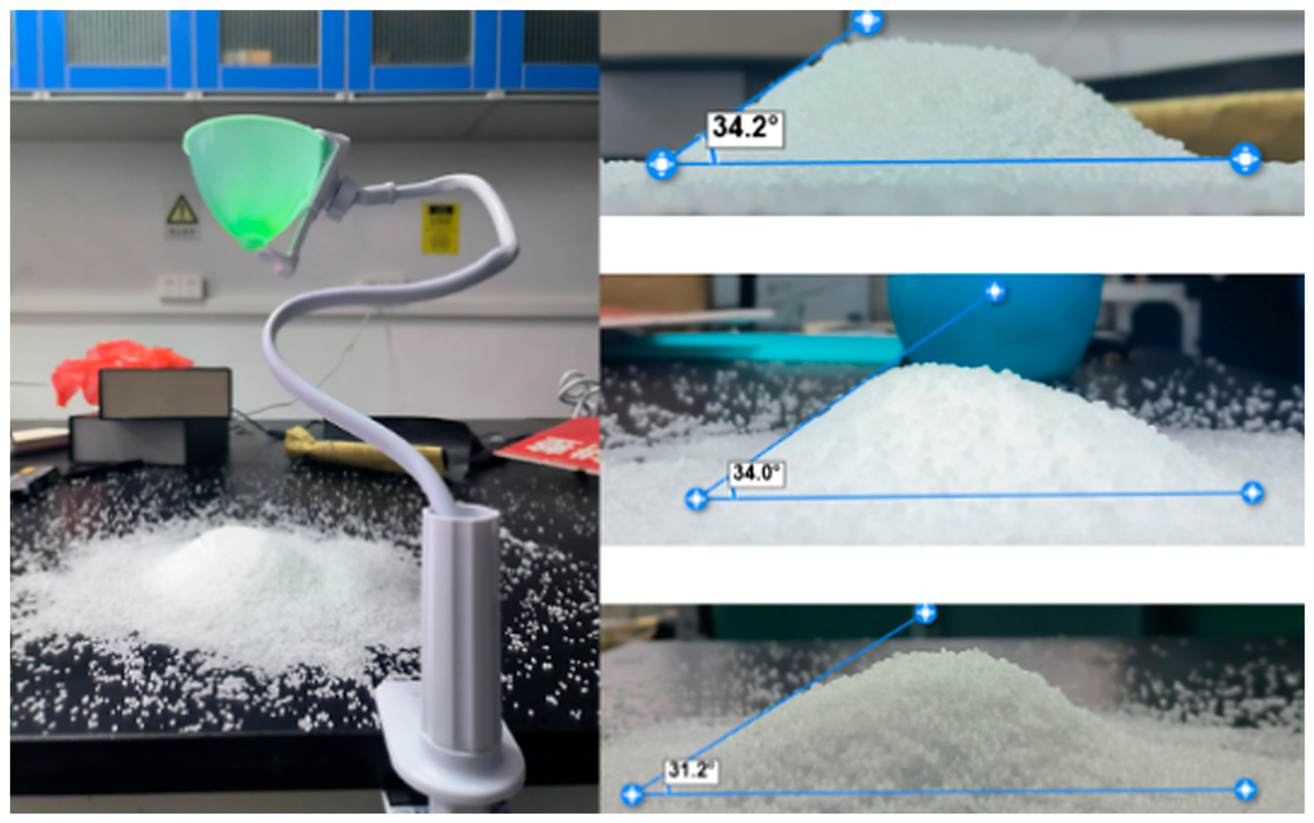
For the physical angle-of-repose test, approximately 500 g of urea was released to form a free pile. After the pile stabilised, photographs were taken from three directions. The background was removed, the pile boundary was extracted, and the slope angle was estimated by least-squares linear fitting in Python 3.9. Three independent trials were conducted, and the mean of the three directional measurements was calculated for each trial (

Table 3. Physical test results for the urea–urea angle of repose.

Trial	Urea–Urea Angle of Repose/°
	Direction 1	Direction 2	Direction 3	Average	Overall Average
1	34.2	34.0	31.2	33.13	33.23
2	33.8	34.6	32.1	33.50
3	31.9	32.7	34.6	33.07

). The overall mean repose angle was 33.23°. The available test record does not include the release height, outlet diameter, or camera distance/resolution; these omissions are treated as methodological limitations. The physical test arrangement is shown in Figure 7.

2.3.2. Urea Sliding Test (Calibration of the Sliding Friction Angle)

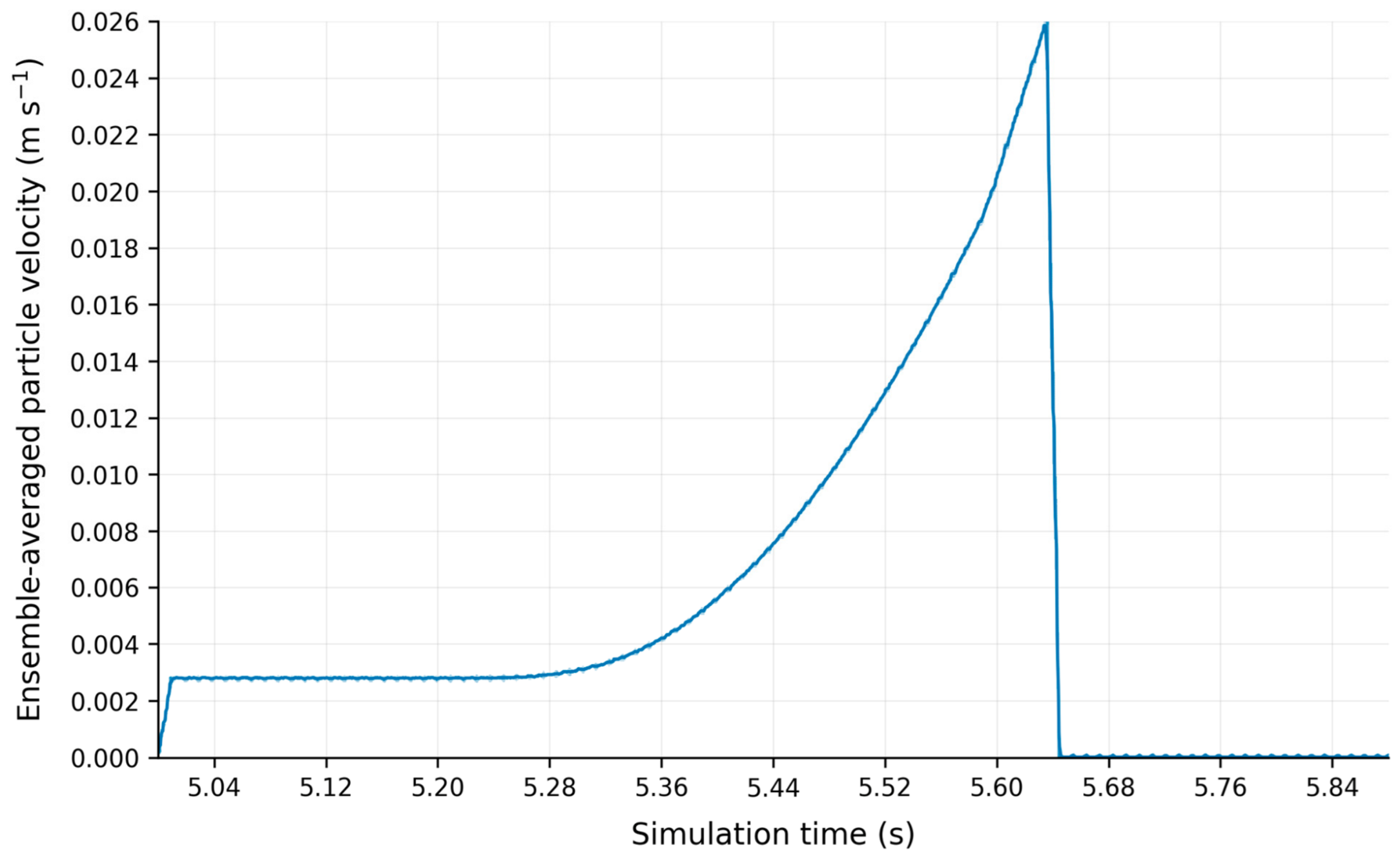
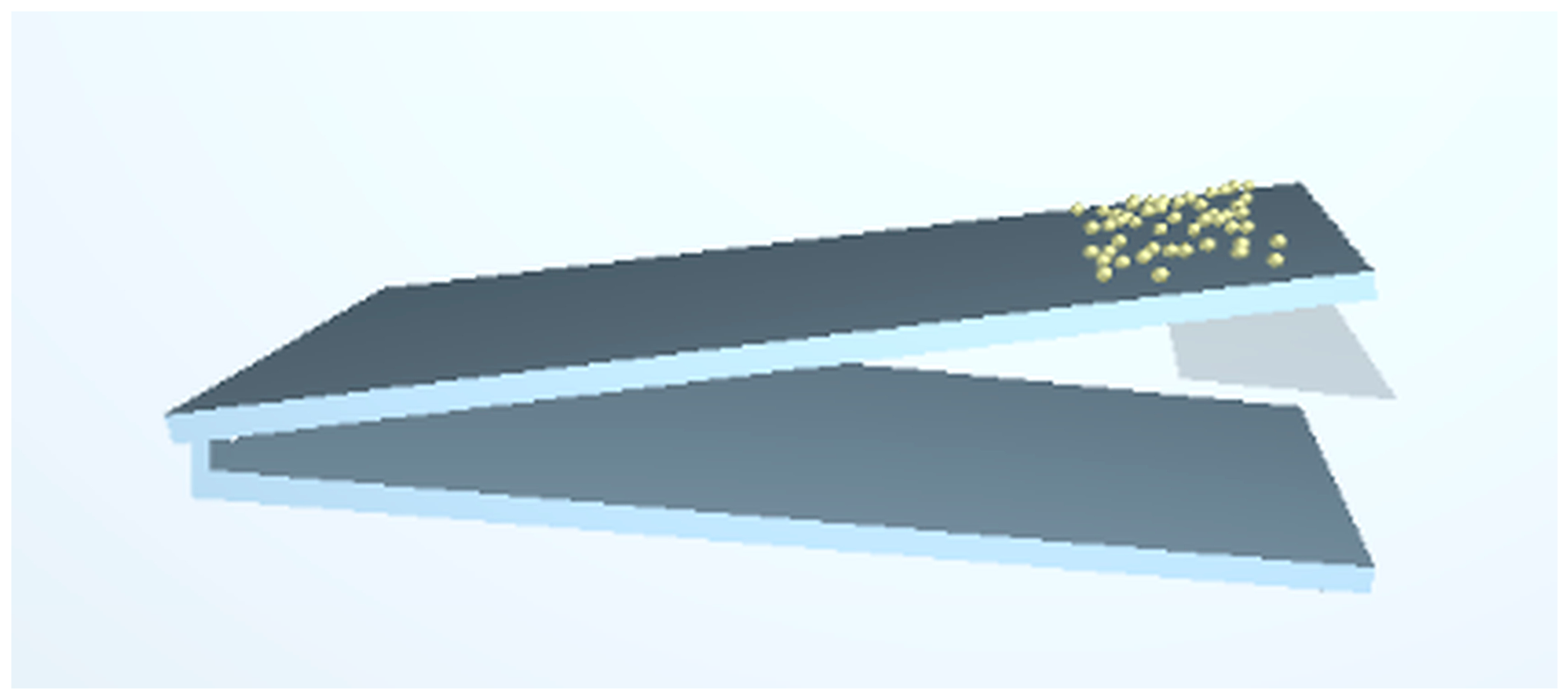
For the sliding simulation, 50 spherical urea particles were generated on a horizontal PP plate at 10 particles·s⁻¹. After the particles became stationary, the plate began rotating about its end hinge at 5 s with an angular velocity of 1 rad·s⁻¹. Sliding onset was identified as the first sustained departure of the ensemble-averaged particle velocity from the stationary baseline, and the corresponding time was converted to the critical inclination angle. Figure 8 and Figure 9 show the simulation model and a representative velocity response. No separate numerical velocity threshold or minimum persistence time was defined for the onset criterion.

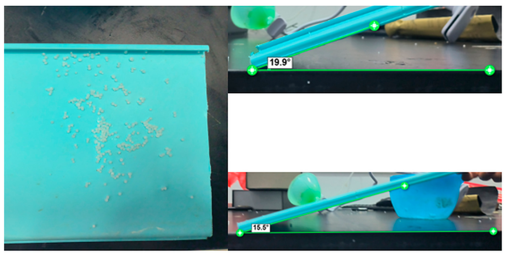
The corresponding physical sliding test used a plate made of the same PP material as the hopper. Approximately 100 g of urea was placed on the plate, which was slowly raised until macroscopic sliding began. The inclination angle at the onset of sliding was determined from the recorded image using a digital image-based protractor. Five independent measurements were obtained, giving a mean sliding friction angle of 15.32° (

Table 4. Physical test results for the urea–PP sliding friction angle.

Trial	1	2	3	4	5	Average/°
Sliding friction angle/°	19.9	15.5	14.0	14.2	13.0	15.32

). The available test record does not include the plate dimensions, surface-roughness preparation, or exact lifting rate. The physical sliding test arrangement is shown in Figure 10.

2.4. DEM Model and Combined Vibration Settings

Sinusoidal translational motion was prescribed to the vibrating boundary. The three operating conditions were a non-vibrating control, 29.17 Hz with 0.2 mm amplitude, and 58.33 Hz with 1.2 mm amplitude. Because frequency and amplitude changed simultaneously, the two vibrating treatments are treated as combined excitation settings. For sinusoidal displacement, x = A sin(2πft), the nominal peak acceleration is (2πf)²A; the two vibrating settings therefore correspond to approximately 6.72 and 161.2 m·s⁻², respectively, a ratio of about 24.

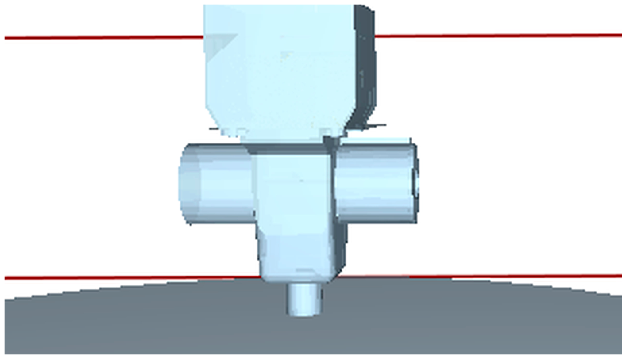
The discharge geometry was created in Creo 7.0 and imported into EDEM 2024. The hopper internal dimensions were 300 mm × 200 mm × 250 mm (length × width × height); the external-fluted metering wheel had a diameter of 80 mm and six flutes, and the discharge outlet diameter was 50 mm. Urea granules were represented as spherical particles with a fixed radius of 0.8475 mm and a particle density of 1236 kg·m⁻³. The original non-JKR vibration/discharge simulations covered 30 s: particle generation occurred at 0–0.5 s, settling and arch development at 0.5–19.5 s, discharge under the assigned excitation at 19.5–25 s, and post-discharge settling at 25–30 s. Dry calibration used Hertz–Mindlin contacts, whereas the separate adhesion-sensitivity simulations used Hertz–Mindlin with JKR for urea–urea contacts together with the Standard Rolling Friction model. The available baseline simulation record does not document the vibration direction. The imported geometric model is shown in Figure 11.

Arch formation was identified qualitatively from persistent particle accumulation above the outlet together with a pronounced decrease in ensemble-averaged particle velocity towards a low, nearly stationary level. Arch failure was identified when the spanning structure visibly collapsed and particle motion and discharge resumed after excitation. Because no numerical velocity or mass-flow threshold was defined, arch formation and failure were assessed qualitatively from particle configuration and velocity response.

The vibration settings were reproduced on the physical test platform. Because frequency and amplitude were not varied independently, the design cannot isolate a frequency effect. The treatments are therefore identified by both frequency and amplitude (29.17 Hz/0.2 mm and 58.33 Hz/1.2 mm), and all comparisons are interpreted as differences between combined excitation settings rather than as effects of frequency alone. No optimum vibration frequency is inferred from these two treatments.

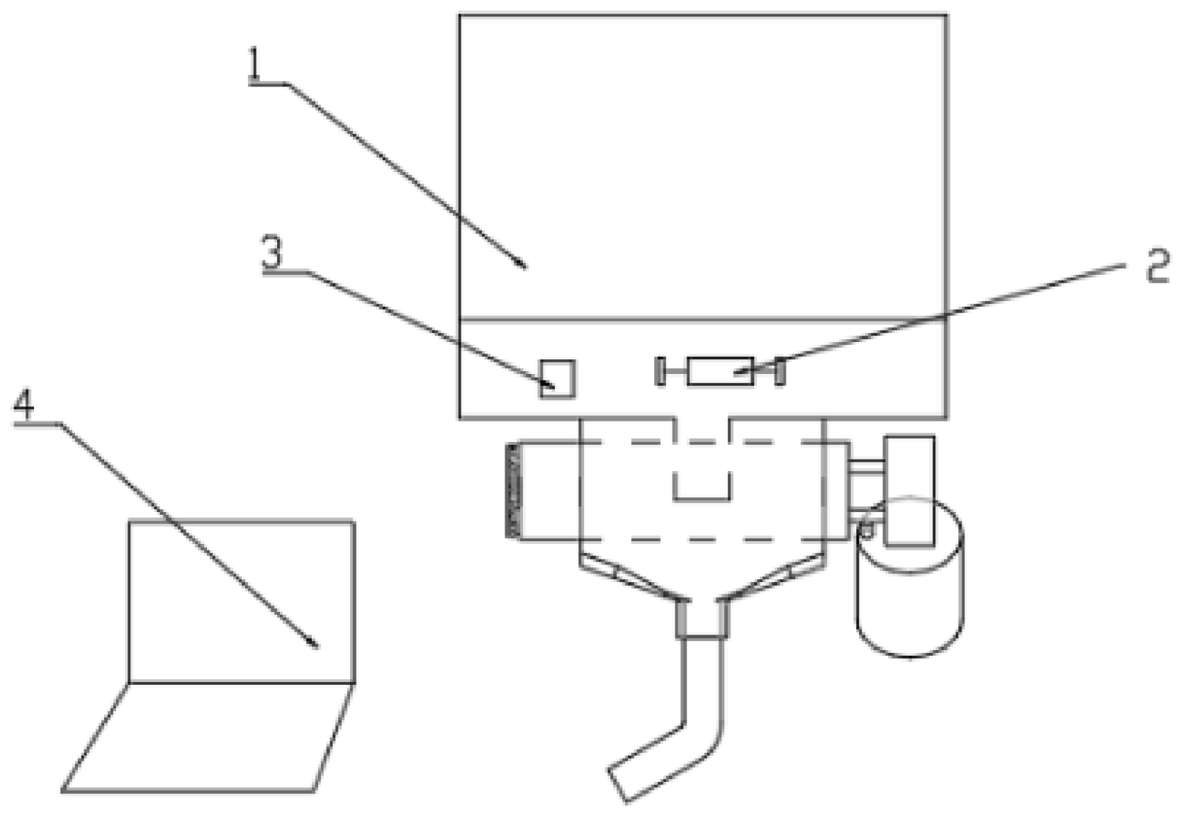
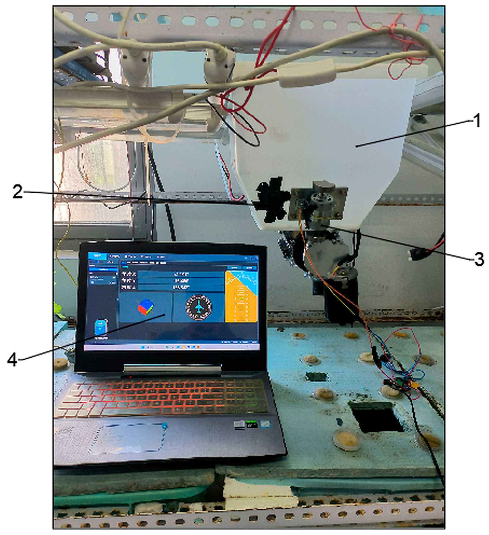
A DC vibration motor (Model 545; Pengyu Precision Co., Ltd., Beijing, China) provided the excitation. Its rated speed of 3500 r·min⁻¹ corresponds to 58.33 Hz, whereas the 1750 r·min⁻¹ operating condition corresponds to 29.17 Hz. A WT9011DCL-BT50 sensor (WitMotion Technology Co., Ltd., China) was mounted on the rig to record acceleration–time data. Vibration amplitude was obtained by double integration of the measured acceleration signal in Origin 2024, yielding 1.2 mm at 58.33 Hz and 0.2 mm at 29.17 Hz (Figure 12 and Figure 13). The test record does not include the sensor sampling frequency, measurement-axis orientation, filtering/windowing settings, or acquisition duration; these omissions are acknowledged as limitations of the vibration measurement.

The JKR simulations were added subsequently as a separate 35 s sensitivity study of prescribed effective adhesion and were independent of the original 30 s non-JKR vibration/discharge simulations. The particle density was 1236 kg·m⁻³, and the fixed spherical particle radius was 0.8475 mm. Hertz–Mindlin with JKR was assigned to urea–urea contacts together with Standard Rolling Friction. Surface energies of 0, 0.05, 0.15, and 0.30 J·m⁻² were prescribed, while all other calibrated material and contact settings were kept unchanged. A virtual dynamic factory generated a target total urea mass of 0.95 kg at 1.9 kg·s⁻¹ from t = 0, corresponding to a nominal generation period of 0.5 s; the factory was mass-controlled, and the exact generated particle count was not recorded separately. Euler integration with Auto Time Step was used. The Rayleigh time step was 1.8782 × 10⁻⁵ s, and the Rayleigh fraction was 20%, corresponding to a displayed computational time step of approximately 3.7564 × 10⁻⁶ s. Each simulation ran for 35 s with a target save interval of 0.01 s using the GPU CUDA solver.

The four JKR surface energy values were selected to span a numerical range from the non-adhesive reference (0 J·m⁻²) to progressively stronger prescribed adhesion. No experimental calibration was available to relate 0.05, 0.15, or 0.30 J·m⁻² quantitatively to urea moisture content, relative humidity, exposure duration, or bulk cohesive strength. Reference [10] supports the occurrence of moisture-assisted bridge formation in urea but does not provide a calibration between these environmental variables and JKR surface energy. Accordingly, the JKR analysis is interpreted strictly as a parametric adhesion-sensitivity study, and no moisture-specific state is assigned to any JKR level.

2.5. Physical Test Rig and Evaluation Metrics

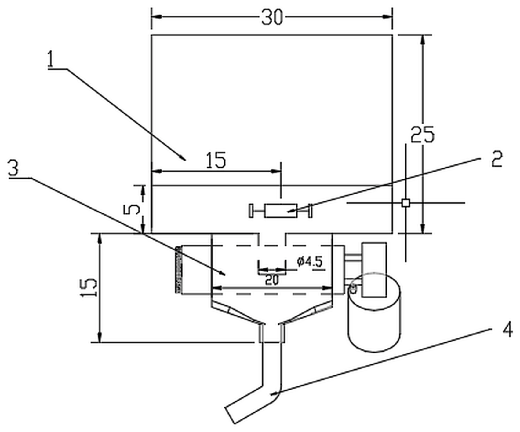
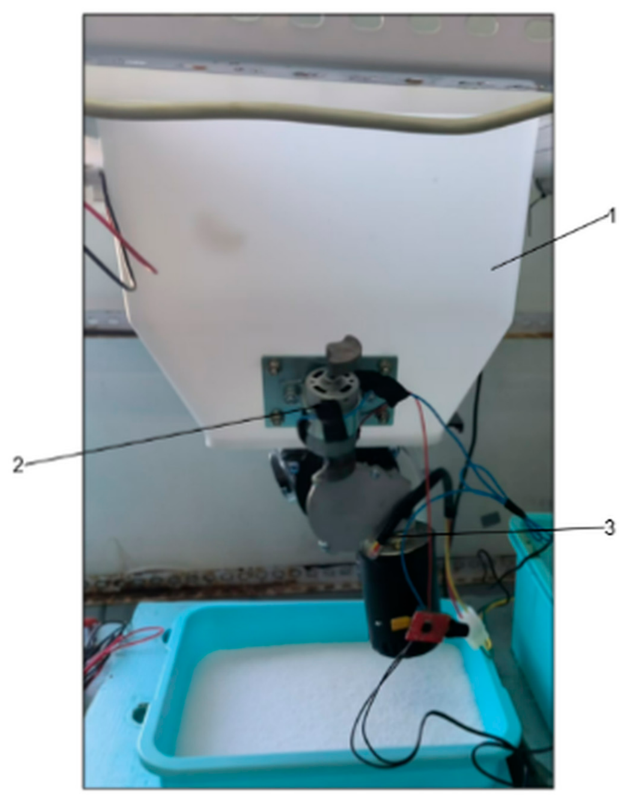
Physical discharge tests were conducted in the F103 laboratory at Jiangsu University using a laboratory-built polypropylene (PP) hopper fabricated at Jiangsu University, Zhenjiang, China, together with the metering and vibration assemblies. The hopper internal dimensions were 300 mm × 200 mm × 250 mm (length × width × height), the external-fluted metering wheel had an 80 mm diameter and six flutes, and the discharge outlet diameter was 50 mm. Figure 14 shows the principal dimensions of the hopper, motor, metering assembly, and discharge chute. The dimensions in Figure 14 are given in centimetres; the principal dimensions are also reported above in millimetres. The assembled physical test rig is shown in Figure 15.

Three treatments were tested: 58.33 Hz/1.2 mm, 29.17 Hz/0.2 mm, and a non-vibrating control. For each replicate, 1.0 kg of urea was loaded into the hopper and left undisturbed for 2–3 min before the 30 s discharge test. This interval was used only to stabilise the granular bed and was not treated as controlled moisture conditioning or as evidence of recrystallised bridge formation. The vibration motor and metering assembly were then operated according to the assigned treatment, and the discharged material was collected and weighed. Twenty replicate runs were performed for each treatment. The experimental records do not include laboratory temperature, relative humidity, initial or final urea moisture content, moisture uptake, the exact metering wheel speed, treatment randomisation, whether fresh or reused urea was used for each replicate, the hopper-cleaning procedure, or an explicit initial-state restoration protocol. These omissions are reported as limitations of the bench experiment.

Because ambient temperature, relative humidity, and urea moisture content were not measured during the bench tests, the physical experiments cannot be quantitatively matched to any prescribed JKR surface energy level.

The coefficient of variation (CV) was used to describe between-run repeatability across the 20 replicate discharge masses. It is not interpreted as a measure of instantaneous temporal or spatial discharge uniformity. The CV was calculated using Equation (5):

$$CV={\displaystyle \frac{\sigma }{m}}\times 100\%$$

(5)

where m denotes the mean collected mass across the 20 replicates, as defined in Equation (6), and σ is the sample standard deviation of the collected mass, as defined in Equation (7):

$$m={\displaystyle \frac{1}{n}}{\displaystyle {\sum }_{i=1}^n}{m}_i$$

(6)

$$\sigma =\sqrt{{\displaystyle \frac{1}{n-1}}{\displaystyle {\sum }_{i=1}^n}{\left(m_i-m\right)}^2}$$

(7)

where mi is the collected discharge mass for replicate i and n is the number of replicates (n = 20).

2.6. Data Processing and Statistical Analysis

For the response surface calibration, the 17-run datasets for angle of repose and sliding friction angle were fitted with full quadratic models. Model significance and lack of fit were evaluated by analysis of variance (ANOVA). Model adequacy was assessed using R², adjusted R², residual standard deviation, model coefficient of variation, the Shapiro–Wilk tests of residual normality, internally studentised residuals, and predicted-versus-observed plots. Full quadratic terms were retained to preserve model hierarchy, and statistical significance was assessed at α = 0.05.

For the bench test datasets, the mean discharged mass, sample standard deviation (SD; denominator n − 1), coefficient of variation (CV = SD/mean × 100%), and 95% confidence interval (CI) of the mean were calculated. Homogeneity of variance was assessed using a mean-centred Levene’s test. Treatment means were compared by one-way analysis of variance (ANOVA), followed by Tukey’s honestly significant difference (HSD) test when the overall ANOVA was significant. Statistical significance was set at α = 0.05. Because the two vibration treatments differed in both frequency and amplitude, statistically significant differences were attributed to the combined treatment settings rather than to frequency alone. The CV was interpreted as between-run repeatability, not as a measure of temporal or spatial uniformity of instantaneous discharge.

3. Results and Discussion

3.1. Calibration Simulation Results and Regression Models

The simulated urea angle of repose (Y₁) and urea–PP sliding friction angle (Y₂) for the 17 response surface design runs are reported in

Table 5. Simulated urea angle of repose (Y₁) for the 17 response surface design runs.

Run	Coefficient of Restitution (X1)	Coefficient of Rolling Friction (X2)	Coefficient of Static Friction (X3)	Angle of Repose/° (Y1)
1	−1	−1	−1	18.9
2	−1	−1	1	29.6
3	−1	1	−1	35.6
4	−1	1	1	52.1
5	1	−1	−1	22.9
6	1	−1	1	21.9
7	1	1	−1	25.8
8	1	1	1	48.4
9	−1.682	0	0	38.4
10	1.682	0	0	36.8
11	0	−1.682	0	17.4
12	0	1.682	0	50.2
13	0	0	−1.682	21.2
14	0	0	1.682	49.2
15	0	0	0	39.3
16	0	0	0	40.3
17	0	0	0	43.9

and

Table 6. Simulated urea–PP sliding friction angle (Y₂) for the 17 response surface design runs.

Run	Coefficient of Restitution (X4)	Coefficient of Rolling Friction (X5)	Coefficient of Static Friction (X6)	Sliding Friction Angle/° (Y2)
1	−1	−1	−1	13.52
2	−1	−1	1	11.80
3	−1	1	−1	18.96
4	−1	1	1	20.57
5	1	−1	−1	11.86
6	1	−1	1	9.40
7	1	1	−1	20.05
8	1	1	1	22.63
9	−1.682	0	0	13.57
10	1.682	0	0	13.23
11	0	−1.682	0	6.76
12	0	1.682	0	23.60
13	0	0	−1.682	13.92
14	0	0	1.682	16.10
15	0	0	0	9.05
16	0	0	0	11.46
17	0	0	0	13.57

, respectively.

The full quadratic models fitted to the data in Table 5 and Table 6 were significant, while the lack-of-fit tests were non-significant (

Table 7. Analysis of variance (ANOVA) for the regression models.

Response	Source of Variance	Sum of Squares	Degrees of Freedom	Mean Square	F-Value	p-Value
	Model	2120.14	9	235.57	14.20	0.001
	X1	28.97	1	28.97	1.75	0.2279
	X2	1121.58	1	1121.58	67.61	<0.0001 **
	X3	673.28	1	673.28	40.59	0.0004 **
	X1X2	12.00	1	12.00	0.7237	0.4231
$Y_1$ Angle of repose	X1X3	3.92	1	3.92	0.2363	0.6417
	X2X3	108.04	1	108.04	6.51	0.0380 *
	X12	44.72	1	44.72	2.70	0.1446
	X22	125.41	1	125.41	7.56	0.0285 *
	X32	90.95	1	90.95	5.48	0.0517
	Lack of Fit	104.41	5	20.88	3.57	0.2333
Sliding friction angle	Model	362.98	9	40.33	14.83	0.0009 **
	X4	0.161	1	0.161	0.059	0.8149
	X5	299.47	1	299.47	110.09	<0.0001 **
	X6	0.990	1	0.990	0.364	0.5654
	X4X5	6.498	1	6.498	2.389	0.1661
	X4X6	0.007	1	0.007	0.002	0.9621
	X5X6	8.757	1	8.757	3.219	0.1159
	X42	11.886	1	11.886	4.370	0.0749
	X52	30.919	1	30.919	11.366	0.0119 *
	X62	28.716	1	28.716	10.556	0.0141 *
	Lack of Fit	8.811	5	1.762	0.345	0.8543

$p<0.01 p<0.05$ Note: ** denotes p < 0.01; * denotes p < 0.05.

). The fitted equations and model diagnostics are summarised below.

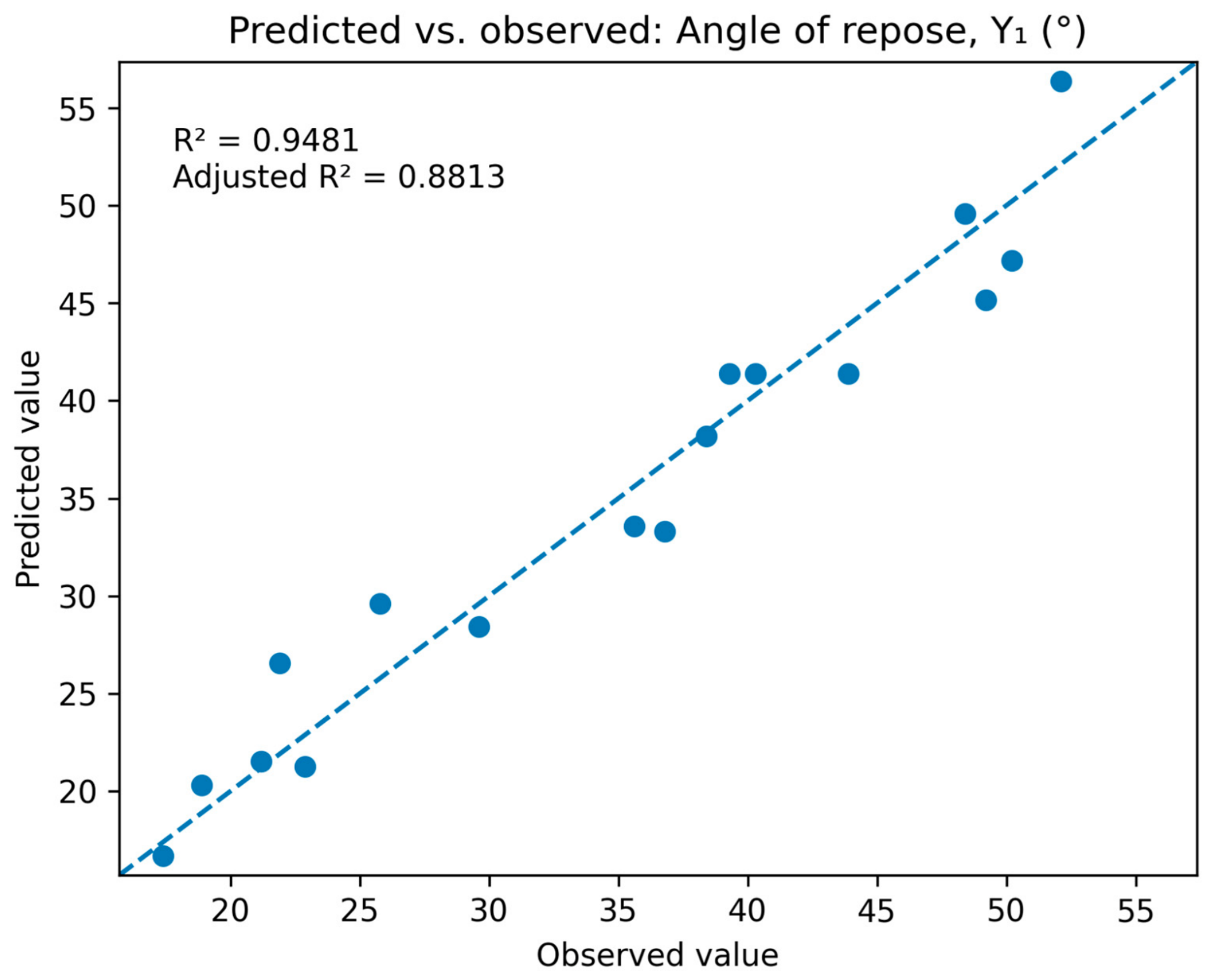
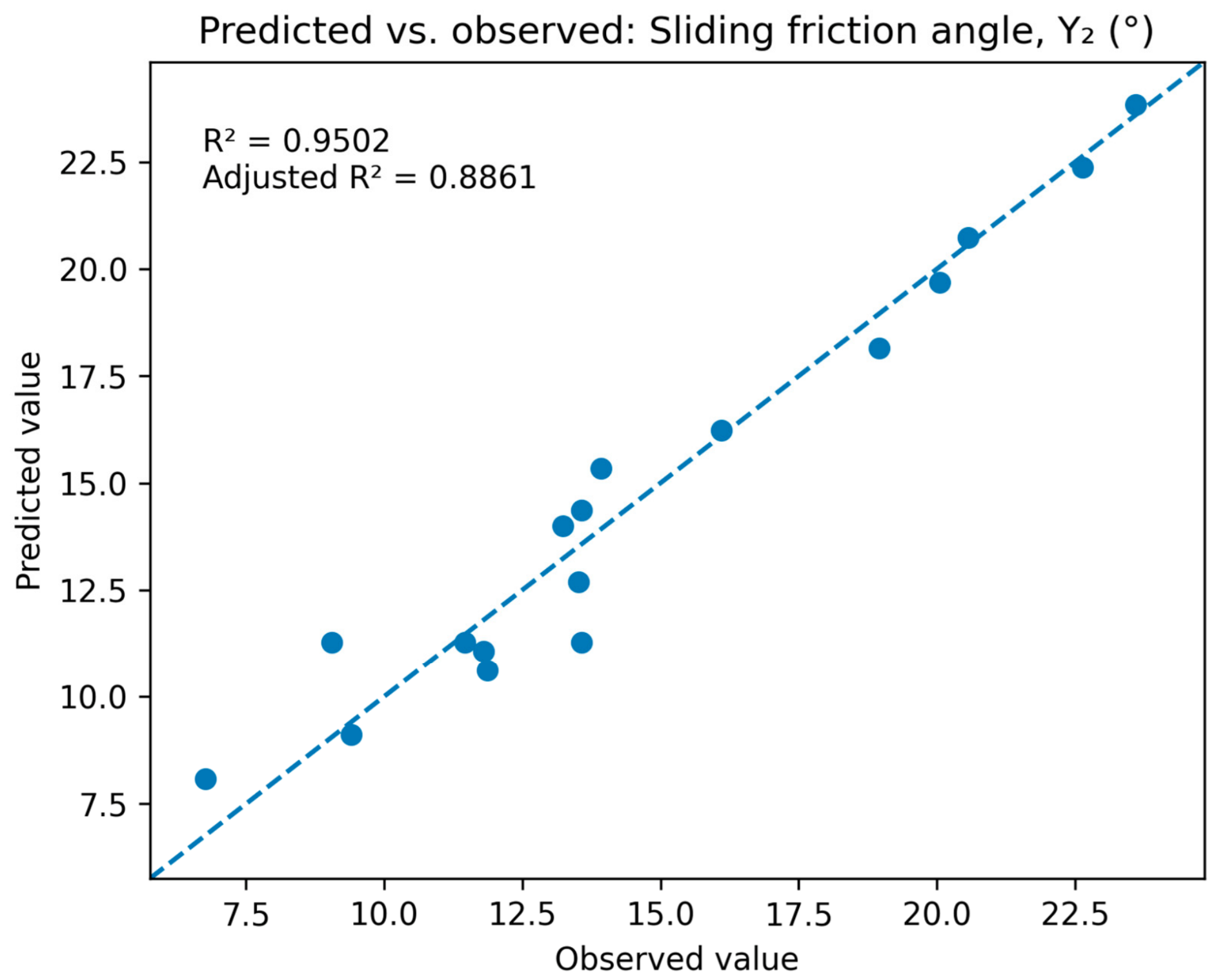
For the angle-of-repose model (Y₁), R² = 0.9481, and adjusted R² = 0.8813; for the sliding angle model (Y₂), R² = 0.9502, and adjusted R² = 0.8861 (

Table 8. Goodness-of-fit parameters for the regression models.

Response	Residual SD	Mean	CV/%	R2	Adjusted R2	Shapiro–Wilk p
Angle of repose	4.07	34.82	11.70	0.9481	0.8813	0.609
Sliding friction angle	1.65	14.71	11.21	0.9502	0.8861	0.973

). The residual standard deviations were 4.07° and 1.65°, respectively. The model CVs describe residual error relative to the response mean and do not indicate experimental reproducibility. The Shapiro–Wilk tests did not reject residual normality (p = 0.609 for Y₁ and p = 0.973 for Y₂), and the largest absolute internally studentised residuals were 1.99 and 1.71, respectively.

Full quadratic models were retained to preserve model hierarchy; statistically non-significant terms were not deleted from Equations (8) and (9). For Y₁, X₂ and X₃ were the dominant linear effects, with X₂X₃ and X₂² also significant at p < 0.05. For Y₂, X₅ was the dominant linear effect, while X₅² and X₆² were significant quadratic terms. The fitted coded factor models are given in Equations (8) and (9).

$$Y_1=41.38-1.46X_1+9.06X_2+7.02X_3-1.23X_1{X}_2-0.70X_1{X}_3+3.67X_2{X}_3-1.99X_1^2-3.34X_2^2-2.84X_3^2$$

(8)

$$Y_2=11.272-0.108X_4+4.683X_5+0.269X_6+0.901X_4{X}_5+0.029X_4{X}_6+1.046X_5{X}_6+1.027X_4^2+1.656X_5^2+1.596X_6^2$$

(9)

Here, X₁, X₂, and X₃ are the coded coefficients of restitution, rolling friction, and static friction for urea–urea contacts, respectively; X₄, X₅, and X₆ are the corresponding coded factors for urea–PP contacts.

Within the tested factor spaces, rolling friction had the strongest fitted effect on both responses. For Y₁, the order of the absolute linear effects was X₂ > X₃ > X₁. For Y₂, X₅ was clearly dominant, whereas the linear effects of X₄ and X₆ were not significant. These rankings apply only to the fitted response surfaces within the tested ranges and should not be interpreted as universal relationships outside those ranges.

Predicted-versus-observed plots were used to assess model agreement visually (Figure 16 and Figure 17). The points were distributed around the 1:1 line without an obvious systematic trend, consistent with the residual diagnostics. Because each response model is based on only 17 design runs, these diagnostics are treated as checks of model adequacy rather than as evidence of general predictive validity.

3.2. Parameter Optimisation and Calibration Consistency Check

Physical measurements yielded a mean angle of repose of 33.23° (Table 3) and a mean sliding friction angle of 15.32° (Table 4).

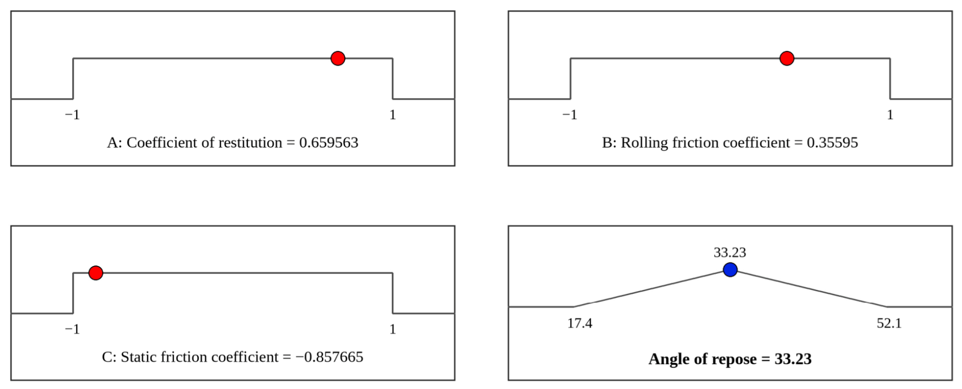
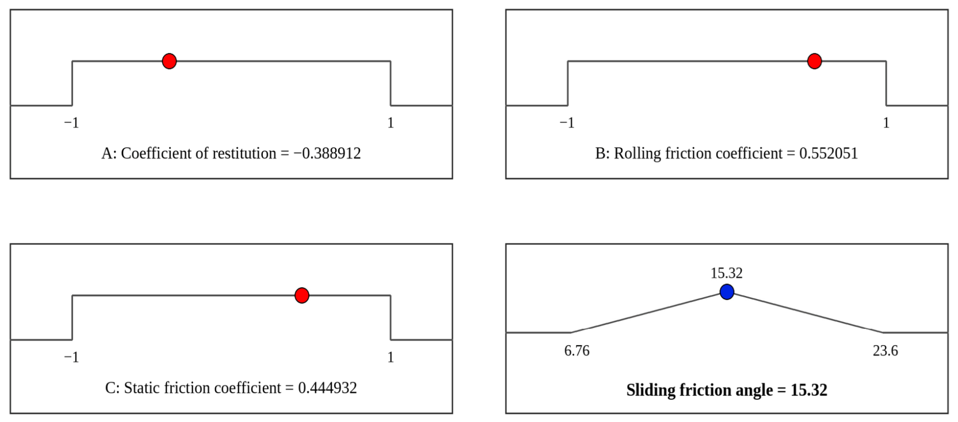
The measured urea–urea angle of repose and urea–PP sliding friction angle were used as optimisation targets in Design-Expert 11.0. Constrained optimisation was performed using the fitted response surfaces (Figure 18 and Figure 19).

The optimal calibrated contact parameter set is presented in

Table 9. Optimised contact parameters.

Calibration Test	Parameter	Code Value	Final Calibrated Value
Urea accumulation test	Coefficient of restitution	0.660	0.39
	Coefficient of rolling friction	0.356	0.49
	Coefficient of static friction	−0.858	0.30
Urea sliding test	Coefficient of restitution	−0.389	0.24
	Coefficient of rolling friction	0.552	0.21
	Coefficient of static friction	0.445	0.57

.

The calibrated parameter set was subsequently applied in EDEM simulations, and the resulting repose and sliding angles were compared with the same physical target measurements used during optimisation. Because these target data are not independent of the calibration process,

Table 10. Simulation–experiment consistency check using the calibrated parameter set.

Assessment Indicator	Simulated Value/°	Experimental Value/°	Relative Error/%
Urea–urea angle of repose	33.80	33.23	1.71
Urea–PP sliding friction angle	15.93	15.32	3.98

is presented as a consistency check rather than as an independent validation.

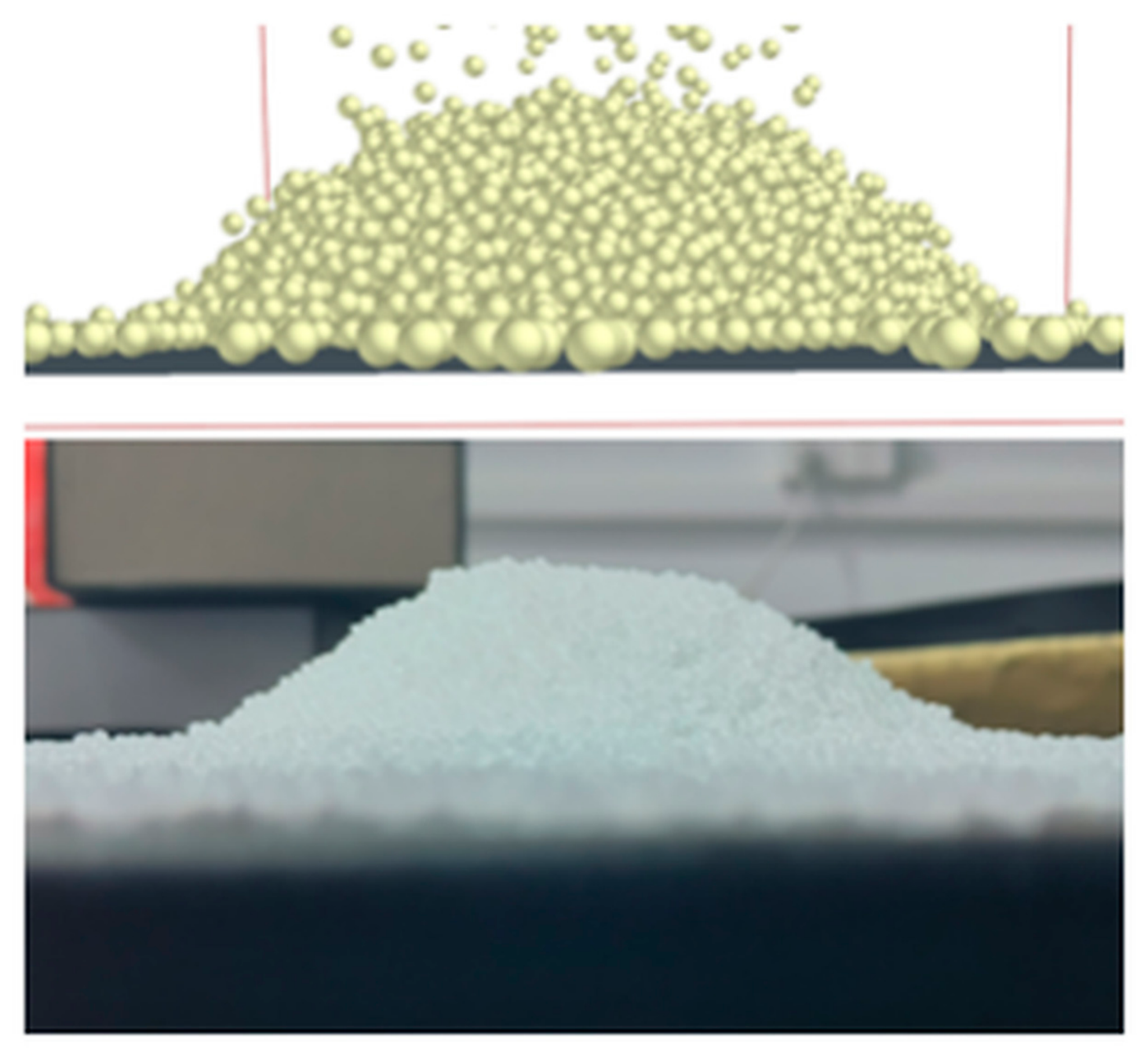
The consistency check simulations yielded a repose angle of 33.80° and a sliding friction angle of 15.93°, corresponding to relative differences of 1.71% and 3.98% from the physical target values, respectively. These small differences indicate internal consistency between the calibrated parameter set and the calibration targets but do not constitute independent external validation. The morphology comparison is shown in Figure 20.

3.3. Simulation Response Under Combined Vibration Excitations

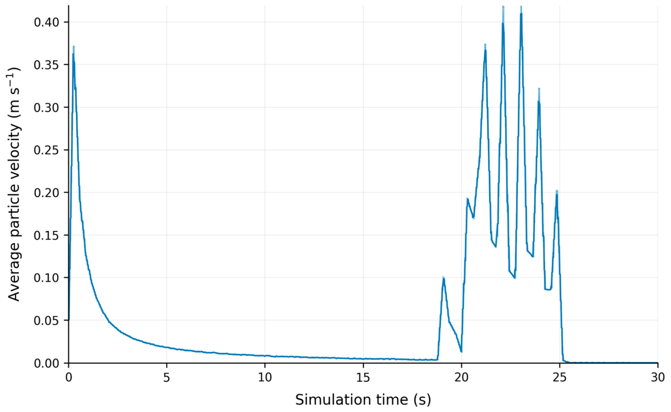
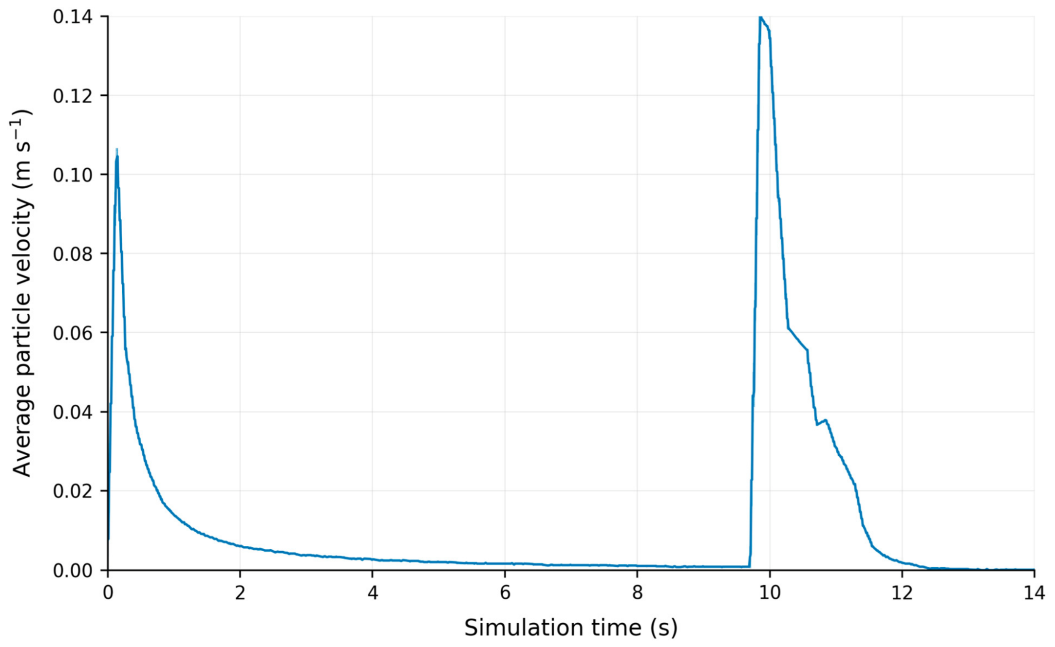
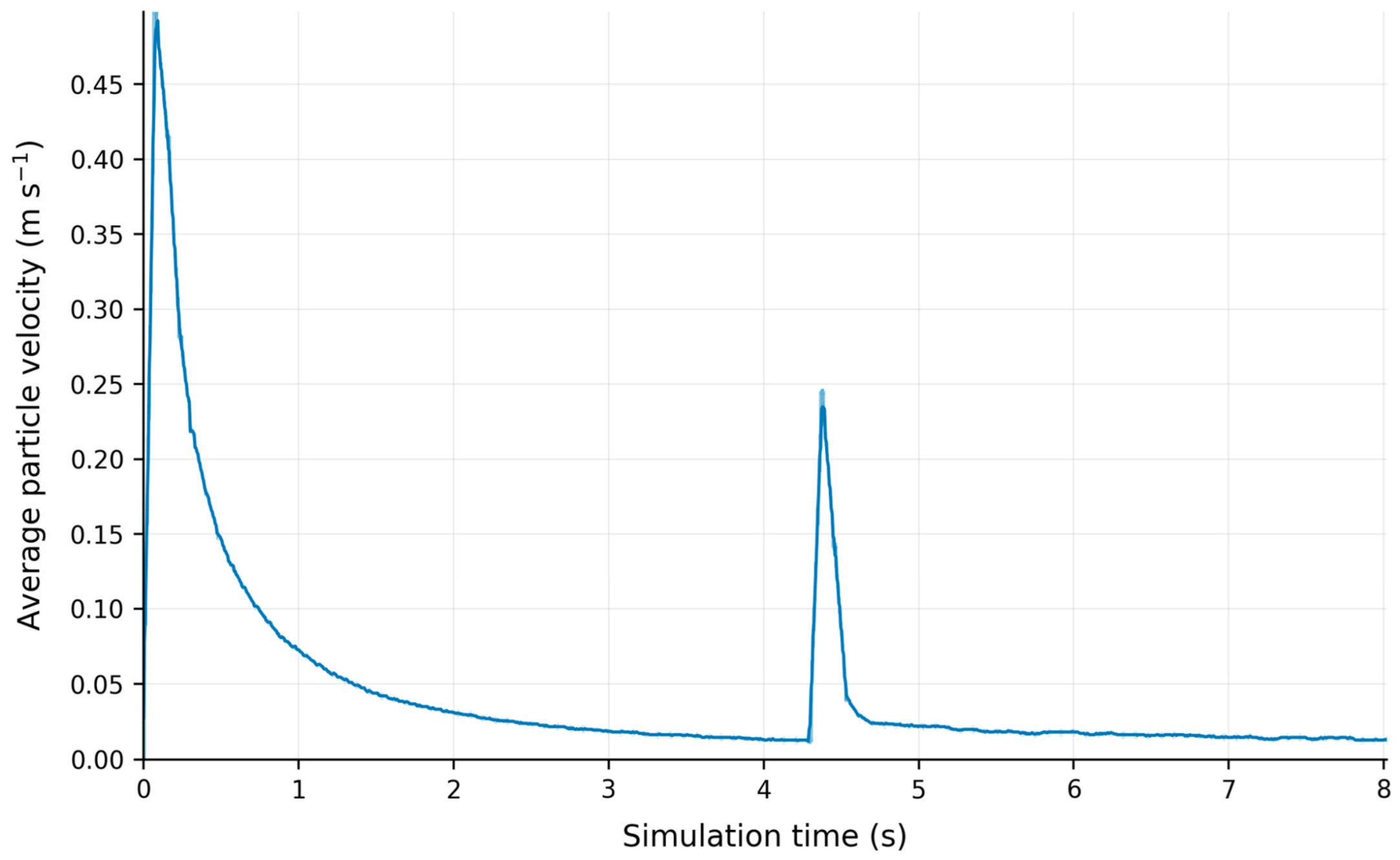
Figure 21, Figure 22 and Figure 23 compare the simulated particle velocity responses under the 58.33 Hz/1.2 mm, 29.17 Hz/0.2 mm, and non-vibrating conditions. Because the two vibrating treatments differ in both frequency and amplitude, they are compared as combined excitation cases. The nominal peak acceleration of the 58.33 Hz/1.2 mm setting is approximately 24 times that of the 29.17 Hz/0.2 mm setting; therefore, the observed response cannot be attributed to frequency alone.

The programmed simulation stages comprised particle generation, settling, outlet opening under the assigned excitation, and post-discharge settling. Arch-like spanning structures, collapse events, and re-arrest were identified from particle configurations and the velocity response as observed phenomena within these stages; they were not prescribed as separate simulation phases.

After the outlet was opened, the vibrating cases exhibited repeated changes in particle velocity, whereas the non-vibrating case approached a near-zero mean velocity. These changes are consistent with repeated rearrangement of the particle network, but the velocity signal alone does not demonstrate microscopic force chain rupture or crystal bridge fracture.

Under the 58.33 Hz/1.2 mm combined excitation, Figure 21 shows the largest and most frequent velocity excursions among the tested conditions. This setting also imposed the larger excitation magnitude: its amplitude was six times greater, and its nominal peak acceleration was approximately 24 times that of the 29.17 Hz/0.2 mm case. The response is therefore interpreted as a combined treatment effect rather than as a frequency effect.

Under the 29.17 Hz/0.2 mm combined excitation, Figure 22 shows smaller velocity fluctuations than under the 58.33 Hz/1.2 mm treatment. This indicates a weaker response under the tested combined setting, but the design does not permit the contributions of frequency and amplitude to be separated.

In the non-vibrating control, Figure 23 shows that the mean particle velocity decreased to approximately zero by 9 s, indicating cessation of bulk discharge in the simulation. This velocity response is not used to infer Bcr > B because the apparent cohesion and bulk unit weight required for a numerical Bcr calculation were not measured.

3.4. JKR Sensitivity Analysis of Prescribed Adhesion

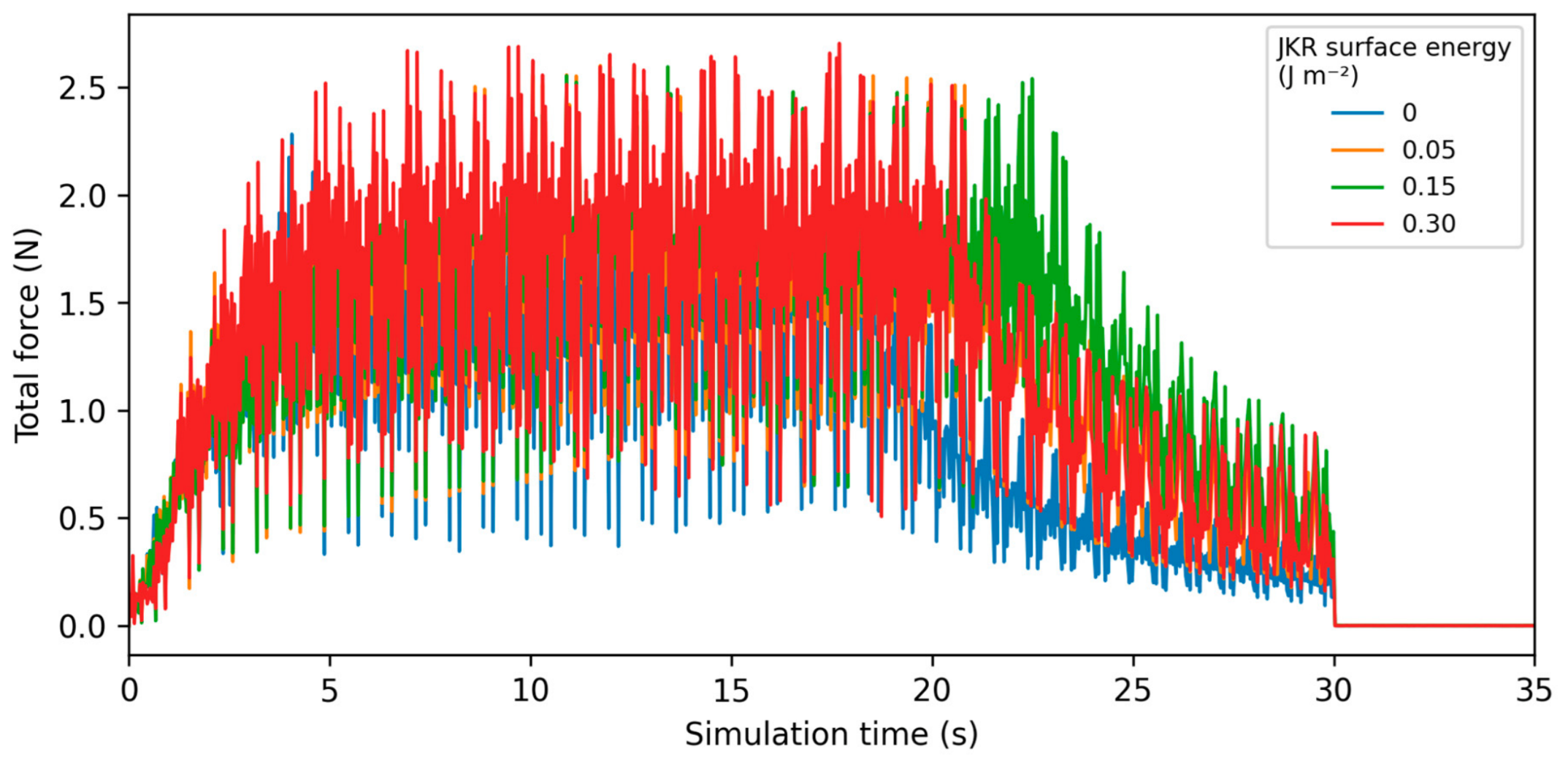
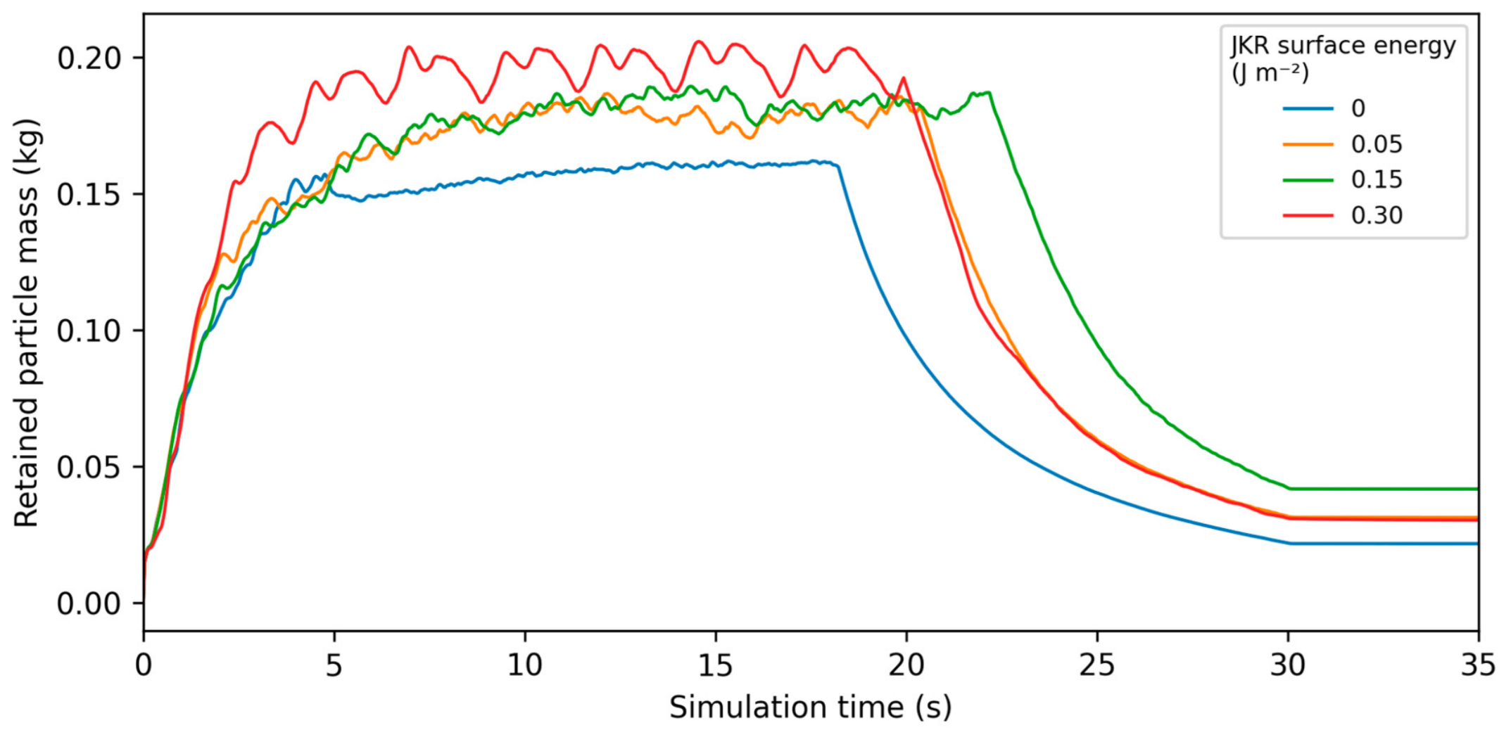
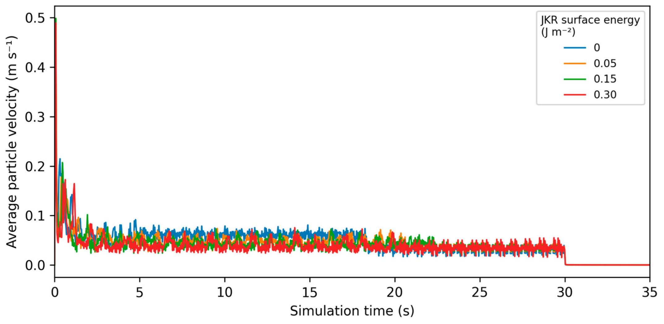
A separate DEM sensitivity analysis varied prescribed JKR surface energy (0, 0.05, 0.15, and 0.30 J·m⁻²) under otherwise fixed discharge settings. The EDEM exports contain time series for the aggregate variable labelled Total Force (N), particle mass (kg) within the monitored hopper region, and average particle velocity (m·s⁻¹) from 0 to 35 s; the corresponding signals are shown in Figure 24, Figure 25 and Figure 26. Total Force is treated as an aggregate post-processing diagnostic for the monitored selection and is not equated with the tensile strength of a specific force chain or crystal bridge. The retained mass trace represents material within the monitored hopper region rather than the total 0.95 kg generated by the particle factory. The available export does not identify whether the monitored region was implemented as a geometry selection or a bin, so no more specific software-region definition is assigned. The surface energy levels are effective adhesion settings and are not mapped to specific moisture contents or relative humidities. A common 5–18 s pre-discharge interval was used to compare particle mobility and mean force level across the four simulations.

The maximum EDEM-exported Total Force values were 2.283, 2.601, 2.596, and 2.704 N for JKR surface energies of 0, 0.05, 0.15, and 0.30 J·m⁻², respectively. The endpoint increase from 0 to 0.30 J·m⁻² was 18.5%. Over the common 5–18 s pre-discharge interval, the mean Total Force values were 1.367, 1.575, 1.602, and 1.708 N, corresponding to an endpoint increase of approximately 25.0%. The nearly identical instantaneous peaks at 0.05 and 0.15 J·m⁻² indicate an overall, but not strictly monotonic, increase in peak force response with prescribed adhesion. Total Force is used only as an aggregate EDEM post-processing diagnostic and is not interpreted as a direct measure of force chain strength or crystal bridge tensile capacity.

The maximum particle mass retained within the monitored hopper region increased from 0.1619 kg at 0 J·m⁻² to 0.1866, 0.1892, and 0.2057 kg at 0.05, 0.15, and 0.30 J·m⁻², respectively. The endpoint increase in this monitored mass signal was approximately 27.0%. These values do not represent the total mass introduced into the JKR simulation: the virtual particle factory generated a target total mass of 0.95 kg. The monitored mass curve therefore describes the time-varying mass within the selected hopper monitoring region and is used only as a relative retention diagnostic. It is also distinct from the 1.0 kg charge used in each physical bench test replicate.

During the common 5–18 s pre-discharge interval, the mean particle velocity decreased systematically from 0.0613 m·s⁻¹ at 0 J·m⁻² to 0.0472, 0.0429, and 0.0397 m·s⁻¹ at 0.05, 0.15, and 0.30 J·m⁻², respectively. The endpoint reduction was approximately 35.3%. The corresponding temporal coefficients of variation increased from 0.131 to 0.203, 0.231, and 0.268, indicating larger relative velocity fluctuations as prescribed adhesion increased. These data indicate reduced particle mobility together with greater relative fluctuations; they do not establish a formal stick–slip regime.

The fixed single-size spherical representation is an important modelling limitation. The measured granules have a finite size distribution, and real urea surfaces are neither perfectly spherical nor smooth. Particle shape and surface morphology can affect packing structure, contact coordination, local contact area, and stress transmission; under humid conditions, they can also influence the locations and effective areas of liquid or recrystallised bridges. Consequently, the absolute arch stability, retained mass, and JKR force response of real granules may differ from those predicted by the idealised spherical model. The JKR results are therefore interpreted as comparative sensitivity trends within the simplified particle representation. Future work should incorporate the measured size distribution and use multi-sphere, polyhedral, or image-reconstructed particle shapes.

The JKR simulations and bench experiments should not be interpreted as tests conducted under matched moisture conditions. The former vary a prescribed numerical adhesion parameter, whereas the latter were conducted without measurements of relative humidity, temperature, moisture uptake, or cohesive strength. The JKR trends therefore support only the qualitative conclusion that stronger prescribed adhesion reduces particle mobility and increases retention and aggregate force response within the model; they do not establish a quantitative relationship between urea moisture state and JKR surface energy.

3.5. Bench Test Results and Statistical Comparison

Table 11. Measured discharge mass under the 58.33 Hz/1.2 mm combined excitation (g).

Replication	1	2	3	4	5
Collected mass/g	534.7	561.9	576.65	581.2	566.9
Replication	6	7	8	9	10
Collected mass/g	575.2	536.3	573.5	524.5	574.4
Replication	11	12	13	14	15
Collected mass/g	542.8	572.5	535.3	586.5	588.6
Replication	16	17	18	19	20
Collected mass/g	590.1	589.7	569.8	578.7	576.9

,

Table 12. Measured discharge mass under the 29.17 Hz/0.2 mm combined excitation (g).

Replication	1	2	3	4	5
Collected mass/g	475.2	510.3	482.5	505.7	468.9
Replication	6	7	8	9	10
Collected mass/g	520.1	478.3	509.9	472.8	515.5
Replication	11	12	13	14	15
Collected mass/g	485.5	499.2	466.5	521.4	489.9
Replication	16	17	18	19	20
Collected mass/g	499.7	472.2	500.8	481.1	493.2

and

Table 13. Measured discharge mass under the non-vibrating control (g).

Replication	1	2	3	4	5
Collected mass/g	492.3	468.77	429.13	453.5	473.2
Replication	6	7	8	9	10
Collected mass/g	477.2	483.2	443.3	424.3	456.3
Replication	11	12	13	14	15
Collected mass/g	468.2	471.3	466.5	477.4	428.3
Replication	16	17	18	19	20
Collected mass/g	465.3	457.9	478.2	488.6	483.2

report the individual discharge masses from 20 replicate runs for each treatment.

The bench test datasets were summarised using the mean, sample SD, 95% CI, and between-run CV and were compared using the inferential procedure described in Section 2.6. The summary statistics are presented in

Table 14. Statistical comparison of discharged mass among the three treatment settings.

Treatment	Mean/g	SD/g	95% CI/g	CV/%	Tukey Group
58.33 Hz/1.2 mm	566.808	20.565	557.183–576.432	3.628	a
29.17 Hz/0.2 mm	492.435	17.630	484.184–500.686	3.580	b
No vibration	464.305	19.980	454.954–473.656	4.303	c

.

The mean-centred Levene’s test provided no evidence of unequal variances among the three treatments (p = 0.919). Treatment had a significant effect on discharged mass (one-way ANOVA: F(2, 57) = 148.54, p < 0.001), and Tukey’s HSD test identified significant pairwise differences among all three treatments (p < 0.001 for each comparison). The 58.33 Hz/1.2 mm condition produced the highest mean discharged mass, 566.808 g (95% CI: 557.183–576.432 g), compared with 492.435 g (484.184–500.686 g) for 29.17 Hz/0.2 mm and 464.305 g (454.954–473.656 g) for the non-vibrating control. Relative to the control, the 58.33 Hz/1.2 mm setting increased the mean discharged mass by approximately 22.1%. The between-run CVs were 3.628%, 3.580%, and 4.303%, respectively. The 29.17 Hz/0.2 mm group had a slightly lower between-run CV than the 58.33 Hz/1.2 mm group, whereas the latter produced the largest mean discharged mass. These CV values are not interpreted as measures of temporal or spatial discharge uniformity.

The bench test used a fixed 30 s collection interval rather than an empty-hopper endpoint. Accordingly, the masses reported in Table 14 represent only the material discharged during 30 s from the 1.0 kg bench test charge. Material remaining in the hopper and metering/discharge path at 30 s was not weighed separately, so a closed experimental mass balance is not available. The approximately 0.16–0.21 kg retained mass signal in Figure 25 belongs to the separate JKR DEM sensitivity simulations, in which the particle factory generated 0.95 kg, and represents mass within the monitored hopper region. It should therefore not be equated with the unmeasured residue from the physical bench tests.

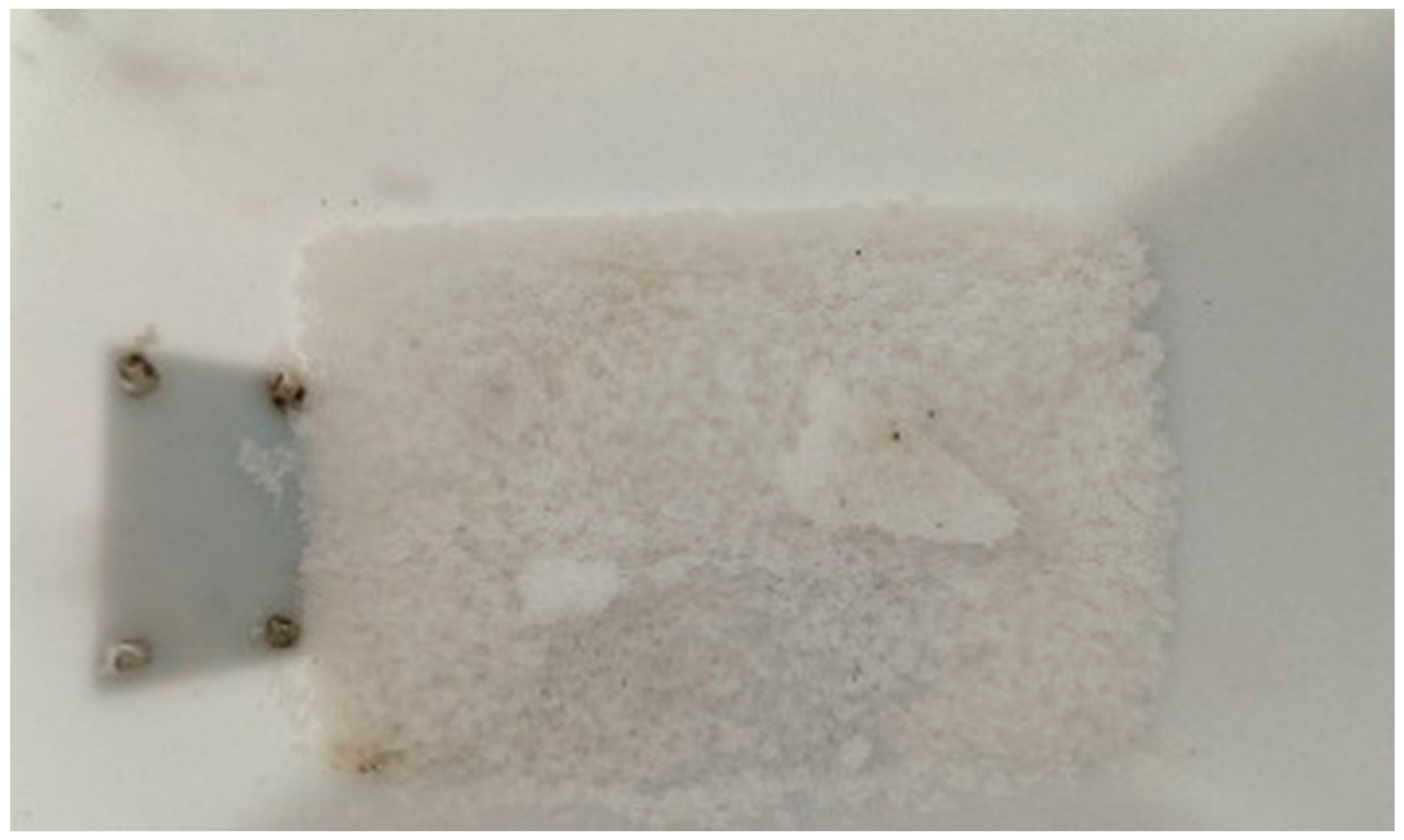
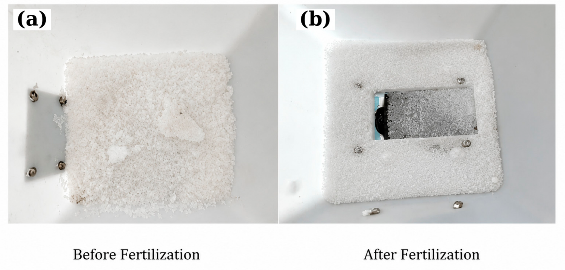
The bench tests therefore show that the 58.33 Hz/1.2 mm combined excitation increased discharged mass under the tested conditions. They do not directly demonstrate fracture of microscopic crystal bridges because bridge structure was not measured and the urea moisture state was not quantitatively characterised. Figure 27 provides a macroscopic before-and-after view of the material configuration.

Taken together, the DEM and bench test results indicate that increasing prescribed adhesion reduces simulated particle mobility, whereas the stronger of the two tested combined vibration settings increases discharged mass. Because frequency and amplitude were confounded and microscopic bridge failure was not measured, the present data neither identify an optimum frequency nor directly demonstrate crystal bridge rupture.

4. Conclusions

Dry-contact calibration produced urea–urea coefficients of restitution, rolling friction, and static friction of 0.39, 0.49, and 0.30, respectively and corresponding urea–PP values of 0.24, 0.21, and 0.57. Applying these parameters in the calibration simulations produced relative differences of 1.71% for the angle of repose and 3.98% for the sliding friction angle compared with the physical target values. In the separate JKR sensitivity analysis, increasing prescribed surface energy from 0 to 0.30 J·m⁻² increased the maximum exported Total Force signal from 2.283 to 2.704 N (18.5%) and reduced mean particle velocity over 5–18 s from 0.0613 to 0.0397 m·s⁻¹ (35.3%). These results describe sensitivity to effective adhesion rather than a calibrated humidity state or direct crystal bridge fracture.

In the bench tests, mean discharged masses were 566.808, 492.435, and 464.305 g for the 58.33 Hz/1.2 mm, 29.17 Hz/0.2 mm, and non-vibrating treatments, respectively. The 58.33 Hz/1.2 mm combined excitation increased the mean mass discharged during the 30 s collection interval by approximately 22.1% relative to the control. The corresponding between-run CVs were 3.628%, 3.580%, and 4.303%. Because frequency and amplitude changed simultaneously, these results demonstrate differences between combined excitation settings rather than an independent frequency effect; the CVs describe repeatability between runs rather than temporal or spatial discharge uniformity.

The principal limitations are the single-size spherical particle representation, the absence of a calibrated relationship between JKR surface energy and urea moisture state, the lack of direct measurements of bridge formation or fracture, and the confounding of vibration frequency with amplitude. Future work should incorporate measured particle-size and shape distributions, controlled humidity conditioning with direct moisture and cohesive strength measurements, calibration of JKR adhesion against those measurements, and factorial vibration experiments in which frequency and amplitude are varied independently. No calibrated moisture threshold or frequency-specific optimum is inferred from the present data.

References

1. Tang, H.; Wang, J.W.; Xu, C.S.; Zhou, W.Q.; Wang, J.F.; Wang, X. Research progress analysis on key technology of chemical fertiliser reduction and efficiency increase. Trans. Chin. Soc. Agric. Mach. 2019, 50, 1–19. (In Chinese) [Google Scholar] [CrossRef]
2. Dong, W.; Wang, S.; Li, H.; Xu, C.; Yu, Q.; Ding, Y. Design and experiment of the self-calibration granular fertiliser detection device for rapeseed mechanized direct seeding. Trans. Chin. Soc. Agric. Eng. 2025, 41, 50–61. (In Chinese) [Google Scholar] [CrossRef]
3. Ding, L.; Xu, Y.F.; Dou, Y.F.; Liu, J.W.; Yu, C.C.; Li, H. Design and experiment of an inclined spiral fertiliser discharge system. Trans. Chin. Soc. Agric. Mach. 2025, 56, 339–348. (In Chinese) [Google Scholar] [CrossRef]
4. Xu, W.; Yuan, Q.; Zeng, J.; Lyu, X. Research progress regarding the precision of dosing and distribution devices for fertilizers. Appl. Sci. 2024, 14, 3059. [Google Scholar] [CrossRef] [Scilit]
5. Liu, X.P.; Jiao, J.; Niu, Z.J.; Du, S.H.; Huang, X.H.; Li, Z.X. Design and experiment of a vibrating organic fertiliser discharging device. J. Chin. Agric. Mech. 2023, 44, 43–50. (In Chinese) [Google Scholar] [CrossRef]
6. Xie, F.P.; Liu, M.Z.; Yang, M.M.; Liu, D.W.; Wang, X.S.; Ren, S.G. Design of ordered fertilizer device for bagged slow-release fertilizer. Trans. Chin. Soc. Agric. Eng. 2019, 35, 40–49. (In Chinese) [Google Scholar] [CrossRef]
7. Wang, B.; Liang, H.; Su, X. Investigation into causes and solutions of compound fertiliser caking. Phosphate Compd. Fertil. 2006, 21, 47–49. (In Chinese) [Google Scholar]
8. Yang, Z.; Tian, Z.; Zhao, H.; Zhao, C.; Zhang, S. Design and application of a four-bar linkage arch-breaking device. Agric. Eng. 2022, 12, 95–100. (In Chinese) [Google Scholar] [CrossRef]
9. Ji, F.; Tong, Y. Analysis of the causes of caking in urea products and corresponding countermeasures. Chem. Fertil. Des. 2008, 46, 40–41. (In Chinese) [Google Scholar]
10. Kirsch, R.M.; Williams, R.A.; Bröckel, U.; Hammond, R.B.; Jia, X. Direct observation of the dynamics of bridge formation between urea prills. Ind. Eng. Chem. Res. 2011, 50, 11728–11733. [Google Scholar] [CrossRef] [Scilit]
11. Liu, X.D.; Ding, Y.C.; Shu, C.X.; Liu, W.P.; Wang, K.Y.; Du, C.Q.; Wang, X.P. Design and experiment of spiral disturbance cone centrifugal fertilizer apparatus. Trans. Chin. Soc. Agric. Eng. 2020, 36, 40–49. (In Chinese) [Google Scholar] [CrossRef]
12. Liu, X.D.; Ding, Y.C.; Shu, C.X.; Wang, K.Y.; Liu, W.P.; Wang, X.P. Analysis and experiment of the disturbance anti-clogging mechanism of a spiral-cone centrifugal fertiliser discharger. Trans. Chin. Soc. Agric. Mach. 2020, 51, 44–54. (In Chinese) [Google Scholar] [CrossRef]
13. Dun, G.Q.; Chen, H.T.; Feng, Y.N.; Yang, J.L.; Li, A.; Zha, S.H. Parameter optimisation and experiment of key components of a fertiliser blending device based on EDEM software. Trans. Chin. Soc. Agric. Eng. 2016, 32, 36–42. (In Chinese) [Google Scholar] [CrossRef]
14. Yang, Q.L.; Wang, Q.J.; Li, H.W.; He, J.; Lu, C.Y.; Yu, C.C.; Lou, S.Y.; Wang, Y.B. Development of layered fertiliser-rate adjustment device for a pneumatic centralised variable-rate fertiliser discharge system. Trans. Chin. Soc. Agric. Eng. 2020, 36, 1–10. (In Chinese) [Google Scholar] [CrossRef]
15. Qi, X.Y.; Zhou, Z.Y.; Yang, C.; Luo, X.W.; Gu, X.Y.; Zang, Y.; Liu, W.L. Design and experiment of key components of a pneumatic variable-rate fertiliser applicator for paddy fields. Trans. Chin. Soc. Agric. Eng. 2016, 32, 20–26. (In Chinese) [Google Scholar] [CrossRef]
16. Li, H.; Wu, J.; Sun, W. Design and experimental evaluation of a vertical layered seeding and fertilising opener. J. Gansu Agric. Univ. 2010, 45, 143–146. (In Chinese) [Google Scholar]
17. Jiang, Y.; He, B.; Lyu, Q.; Zhang, L.; Liu, Y. optimisation analysis and discrete-element simulation of soil–straw mixed accumulation in a smokeless plant-ash furnace. J. Chin. Agric. Mech. 2025, 46, 235–241. (In Chinese) [Google Scholar] [CrossRef]
18. Lu, Q.; Liu, F.; Liu, L.; Liu, Z.; Liu, Y. Establishment and validation of a discrete-element interaction model for furrow soil, seeds, and a soil-covering device. Trans. Chin. Soc. Agric. Mach. 2023, 54, 46–57. (In Chinese) [Google Scholar] [CrossRef]
19. Wang, D.; Lu, T.; Zhao, Z.; Shang, S.; Zheng, S. Calibration method of discrete element simulation parameters for tillage-layer soil in coastal saline–alkali land. Trans. Chin. Soc. Agric. Mach. 2024, 55, 240–249. (In Chinese) [Google Scholar] [CrossRef]
20. Zhao, Z.; Wu, M.; Xie, S.; Luo, H.; Li, P.; Zeng, Y.; Jiang, X. Calibration of discrete-element simulation parameters for soil–rice-stubble mixtures and analysis of rotary-tillage trajectories. Trans. Chin. Soc. Agric. Eng. 2024, 40, 72–82. (In Chinese) [Google Scholar] [CrossRef]
21. Song, S.L.; Tang, Z.H.; Zheng, X.; Liu, J.B.; Meng, X.J.; Liang, Y.C. Calibration of discrete-element parameters for a post-tillage soil model in Xinjiang cotton fields. Trans. Chin. Soc. Agric. Eng. 2021, 37, 63–70. (In Chinese) [Google Scholar] [CrossRef]
22. Xing, X.; Ma, X.; Chen, L.; Li, H.; Wen, Z.; Zeng, G. Experimental investigation of the physical properties of solid granular fertilizers. J. Agric. Mech. Res. 2020, 42, 125–130. (In Chinese) [Google Scholar] [CrossRef]
23. Yuan, F.; Wang, L.; Shi, Y.; Wang, X.; Wang, F.; Liu, H. Mechanical property parameters of fertiliser granules for variable-rate fertiliser spreaders. Tract. Farm Transp. 2022, 49, 51–56. (In Chinese) [Google Scholar]
24. Bu, H.; Yu, S.; Dong, W.; Wang, Y.; Zhang, L.; Xia, Y. Calibration and testing of discrete element simulation parameters for urea particles. Processes 2022, 10, 511. [Google Scholar] [CrossRef] [Scilit]
25. Zhao, J.J.; Han, J.; Han, H.; Liu, S.Q.; Liao, H.H.; Qu, X.R.; Zhang, T.Y. Calibration of simulation parameters between granular fertilizers and PVC plates based on the discrete element method. J. Agric. Mech. Res. 2024, 46, 54–58. (In Chinese) [Google Scholar] [CrossRef]
26. Liu, C.L.; Li, Y.N.; Song, J.N.; Ma, T.; Wang, M.M.; Wang, X.J.; Zhang, C. Performance analysis and experiment of a centrifugal-disc fertiliser spreader based on EDEM. Trans. Chin. Soc. Agric. Eng. 2017, 33, 32–39. (In Chinese) [Google Scholar] [CrossRef]
27. Kumar, M.; Gaur, K.K.; Shakher, C. Measurement of material constants (Young’s modulus and Poisson’s ratio) of polypropylene using digital speckle pattern interferometry (DSPI). J. Jpn. Soc. Exp. Mech. 2015, 15, s87–s91. [Google Scholar] [CrossRef]
28. Wang, J.; Zou, D.; Wang, J.; Zhou, W. Testing and analysis of the shear modulus of urea granules. In Computer and Computing Technologies in Agriculture VII; Li, D., Chen, Y., Eds.; IFIP Advances in Information and Communication Technology; Springer: Berlin/Heidelberg, Germany, 2014; Volume 419, pp. 137–144. [Google Scholar] [CrossRef] [Scilit]
29. Zhang, R.; Han, D.L.; Ji, Q.L.; He, Y.; Li, J.Q. Calibration method for sand parameters in discrete-element simulation. Trans. Chin. Soc. Agric. Mach. 2017, 48, 49–56. (In Chinese) [Google Scholar] [CrossRef]
30. Ma, S.; Xu, L.M.; Yuan, Q.C.; Niu, C.; Zeng, J.; Chen, C.; Wang, S.S.; Yuan, X.T. Calibration of discrete-element simulation parameters for interactions between grapevine cold-proof soil and soil-clearing components. Trans. Chin. Soc. Agric. Eng. 2020, 36, 40–49. (In Chinese) [Google Scholar] [CrossRef]
31. Ou, M.; Wang, G.; Lu, Y.; Zhang, Z.; Pan, H.; Jia, W.; Dong, X. Structure optimisation and performance simulation of a double-disc fertiliser spreader based on EDEM-CFD. Agronomy 2025, 15, 1025. [Google Scholar] [CrossRef] [Scilit]
32. Shi, J.; Hu, J.; Li, J.; Liu, W.; Yue, R.; Zhang, T.; Yao, M. Design and experiment of planting mechanism of automatic transplanter for densely planted vegetables. Agriculture 2024, 14, 1357. [Google Scholar] [CrossRef] [Scilit]
33. Liu, Y.; Li, Y.; Chen, L.; Zhang, T.; Liang, Z.; Huang, M.; Su, Z. Study on performance of concentric threshing device with multi-threshing gaps for rice combines. Agriculture 2021, 11, 1000. [Google Scholar] [CrossRef] [Scilit]
34. Song, X.; Li, H.; Chen, C.; Xia, H.; Zhang, Z.; Tang, P. Design and experimental testing of a control system for a solid-fertiliser-dissolving device based on fuzzy PID. Agriculture 2022, 12, 1382. [Google Scholar] [CrossRef] [Scilit]
35. Hou, T.; Chen, X.; Hu, J.; Liu, W.; Lv, J.; Tan, Y.; Li, F. Design and experimental research on an automated force-measuring device for plug seedling extraction. Agriculture 2025, 15, 1939. [Google Scholar] [CrossRef] [Scilit]
36. Yuan, H.; Liang, S.; Wang, J.; Lu, Y. Numerical simulation and analysis of vibrating rice filling based on EDEM software. Agriculture 2022, 12, 2013. [Google Scholar] [CrossRef] [Scilit]
37. Liu, W.; Hu, J.; Yao, M.; Zhao, J.; Lakhiar, I.A.; Lu, C.; Pan, H.; Wang, W. Magnetic field distribution simulation and performance experiment of a magnetic seed-metering device based on the combined magnetic system. Int. J. Agric. Biol. Eng. 2021, 14, 108–117. [Google Scholar] [CrossRef] [Scilit]
38. Yuan, H.; Wang, H.; Huang, J.; Li, L.; Peng, S.; Wang, J. Study on uniformity of linear vibrating rice feeding device with matrix-designed outlets based on discrete element method. J. Food Eng. 2024, 381, 112170. [Google Scholar] [CrossRef] [Scilit]
39. Wang, X.; Li, Y.; Bai, J. Simulation and experimental study on vibration separation of residual film and soil based on EDEM. Agriculture 2025, 15, 1987. [Google Scholar] [CrossRef] [Scilit]
40. Zhao, Z.; Jin, M.; Tian, C.; Yang, S.X. Prediction of seed distribution in rectangular vibrating tray using grey model and artificial neural network. Biosyst. Eng. 2018, 175, 194–205. [Google Scholar] [CrossRef] [Scilit]
41. Gao, P.; Liu, X.; Xu, Z.; Wang, S.; Qu, M.; Ma, Y. DEM simulation and experimental investigation of draft-reducing performance of up-cutting subsoiling method inspired by animal digging. Agriculture 2025, 15, 2046. [Google Scholar] [CrossRef] [Scilit]
42. Dai, Q.; Zuo, Z.; Zheng, Q.; Fu, Y.; Zhang, S.; Mao, H. optimisation and experimental study of a soil-loosening and root-lifting device for Shanghai Green (Brassica rapa subsp. chinensis) harvesting based on an EDEM–RecurDyn simulation. Agriculture 2025, 15, 1865. [Google Scholar] [CrossRef] [Scilit]
43. Bielykh, O.; Kharchenko, O. Development of an Analytical Model for Predicting the Trajectory and Energy Dissipation of Bee Bread Granules in a Rotary Impact Separator. Technol. Audit Prod. Reserves 2026, 1, 23–31. [Google Scholar] [CrossRef] [Scilit]
44. Kuts, A.; Troyanovskaya, I.; Orekhovskaya, A.; Tikhonov, E.; Sokolova, V. Transporting Ability Calculation of the Rotor of Soil-Cultivating Loosening and Separating Vehicle. Acta Technol. Agric. 2022, 25, 73–78. [Google Scholar] [CrossRef] [Scilit]
Figure 1. Urea arching inside the fertiliser hopper.
Agronomy 16 01728 g001
Figure 2. Representative micrographs of intergranular crystal bridges between urea prills: (A) left-hand micrograph; (B) right-hand micrograph. Reprinted with permission from Ref. [10]. Copyright 2011 American Chemical Society; RightsLink Licence No. 6123531209157.
Agronomy 16 01728 g002
Figure 3. Static analysis model of urea arching: (a) overall geometric model of hopper arching; (b) force model of the half-arch free body.
Agronomy 16 01728 g003
Figure 4. Conceptual schematic of particle–bridge contact mechanics.
Agronomy 16 01728 g004
Figure 5. Conceptual schematic of the arch geometry used in the idealised stress relation; Equation (4) is given only in the main text.
Agronomy 16 01728 g005
Figure 6. Redrawn schematic of the angle-of-repose measurement applied to the stationary EDEM pile profile.
Agronomy 16 01728 g006
Figure 7. Physical angle-of-repose test for urea granules.
Agronomy 16 01728 g007
Figure 8. Simulation model of the urea sliding test.
Agronomy 16 01728 g008
Figure 9. Average particle velocity response during the sliding simulation (x-axis: simulation time, s; y-axis: ensemble-averaged particle velocity, m·s−1).
Agronomy 16 01728 g009
Figure 10. Physical sliding friction test using the polypropylene (PP) plate.
Agronomy 16 01728 g010
Figure 11. Geometric model of the fertiliser discharger used in the DEM simulation.
Agronomy 16 01728 g011
Figure 12. Schematic of the vibration test setup for the fertiliser discharger (1, hopper; 2, vibration motor; 3, WT9011DCL-BT50 sensor; 4, data terminal).
Agronomy 16 01728 g012
Figure 13. Physical setup for vibration measurement under operating conditions (1, hopper; 2, WT9011DCL-BT50 sensor; 3, vibration motor; 4, data terminal).
Agronomy 16 01728 g013
Figure 14. Geometric configuration and principal dimensions of the fertiliser discharger (1, hopper; 2, excitation motor; 3, electric volumetric metering box; 4, discharge chute). The dimensions in the schematic are in centimetres; the principal dimensions are also reported in the text in millimetres.
Agronomy 16 01728 g014
Figure 15. Physical test rig for the vibratory fertiliser discharge experiment (1, hopper; 2, excitation motor; 3, electric volumetric metering box).
Agronomy 16 01728 g015
Figure 16. Predicted versus observed angle of repose (Y1) for the full quadratic regression model. Blue dots represent the predicted–observed data pairs, and the dashed line denotes the 1:1 reference line.
Agronomy 16 01728 g016
Figure 17. Predicted versus observed sliding friction angle (Y2) for the full quadratic regression model. Blue dots represent the predicted–observed data pairs, and the dashed line denotes the 1:1 reference line.
Agronomy 16 01728 g017
Figure 18. Target optimisation analysis for urea–urea angle of repose. Red dots indicate the selected coded factor levels, and the blue dot indicates the target response value.
Agronomy 16 01728 g018
Figure 19. Target optimisation analysis for urea–PP sliding friction angle. Red dots indicate the selected coded factor levels, and the blue dot indicates the target response value.
Agronomy 16 01728 g019
Figure 20. Comparison of simulated and experimental urea pile morphologies.
Agronomy 16 01728 g020
Figure 21. Particle velocity response under the 58.33 Hz/1.2 mm combined excitation (x-axis: simulation time, s; y-axis: average particle velocity, m·s−1).
Agronomy 16 01728 g021
Figure 22. Particle velocity response under the 29.17 Hz/0.2 mm combined excitation (x-axis: simulation time, s; y-axis: average particle velocity, m·s−1).
Agronomy 16 01728 g022
Figure 23. Particle velocity response under the non-vibrating control (x-axis: simulation time, s; y-axis: average particle velocity, m·s−1).
Agronomy 16 01728 g023
Figure 24. EDEM-exported Total Force response at the prescribed JKR surface energy levels.
Agronomy 16 01728 g024
Figure 25. Particle mass retained within the monitored hopper region at the prescribed JKR surface energy levels.
Agronomy 16 01728 g025
Figure 26. Average particle velocity response at the prescribed JKR surface energy levels.
Agronomy 16 01728 g026
Figure 27. Macroscopic material configuration in the hopper: (a) before the discharge test; (b) after the discharge test. The exact acquisition time of panel (b) was not recorded in the experimental records.
Agronomy 16 01728 g027