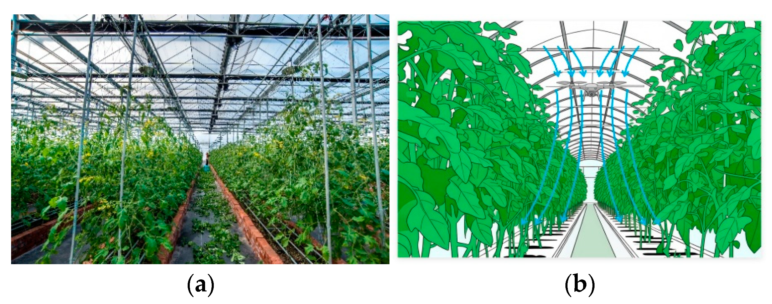
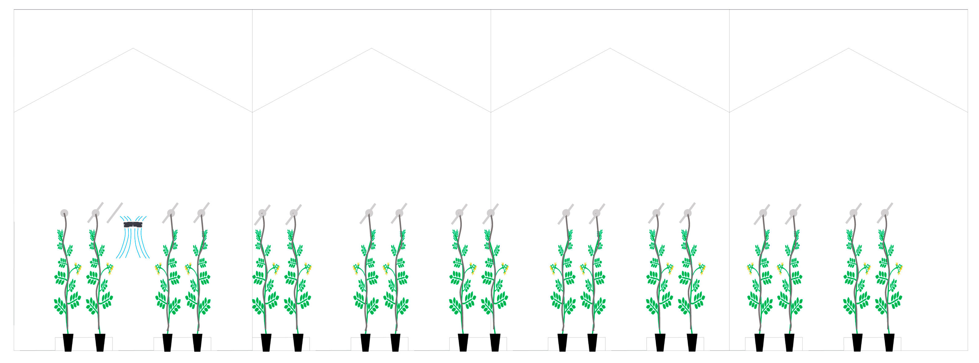
Figure 1.
Schematic diagram of a greenhouse tomato cultivation scene and the distribution of the drone’s downwash flow field. (a) Schematic diagram of greenhouse tomato cultivation; (b) Schematic diagram of the distribution of the downwash flow field from a drone.
Figure 1.
Schematic diagram of a greenhouse tomato cultivation scene and the distribution of the drone’s downwash flow field. (a) Schematic diagram of greenhouse tomato cultivation; (b) Schematic diagram of the distribution of the downwash flow field from a drone.
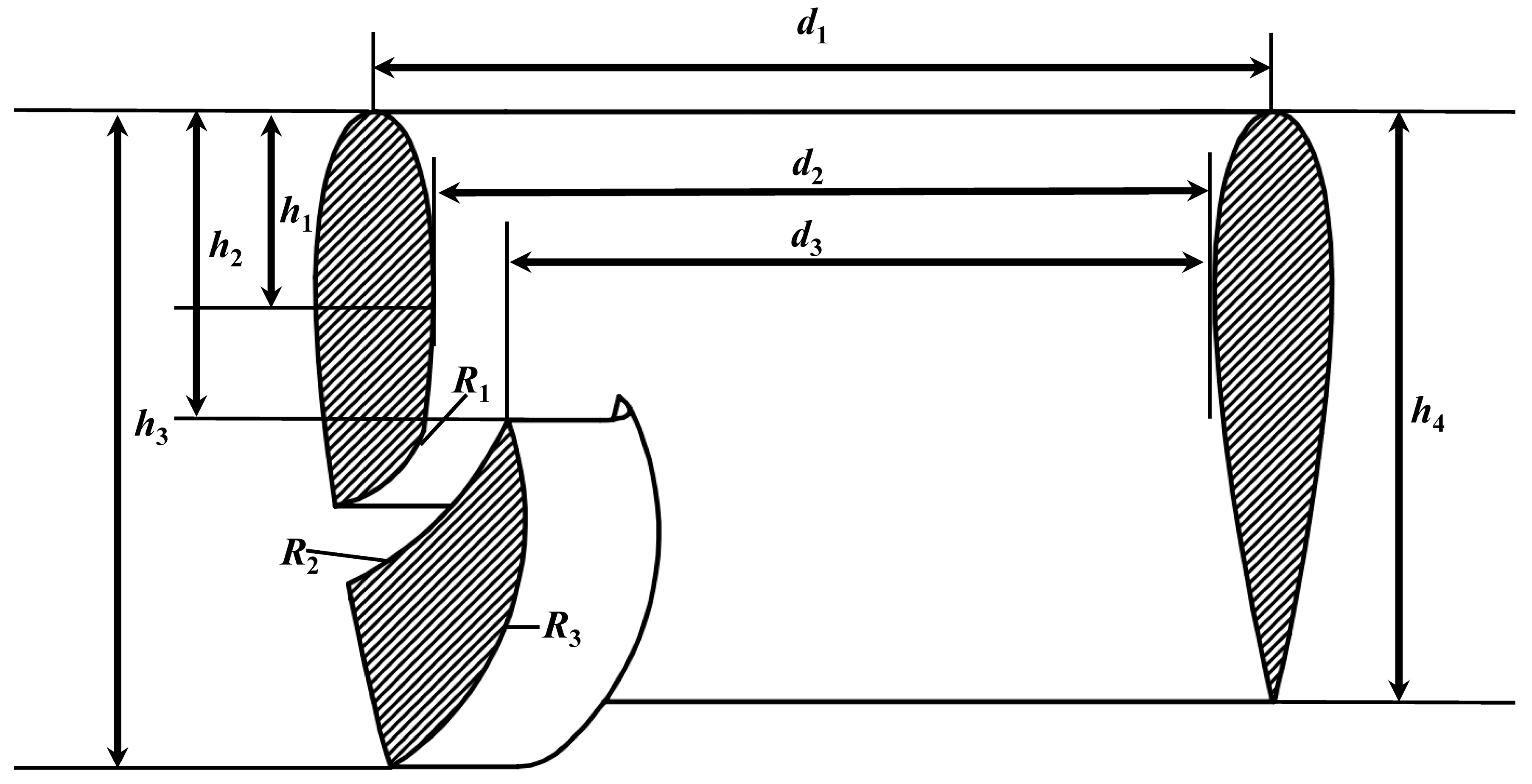
Figure 2.
Schematic diagram of the asymmetric duct structure and parameter definitions.
Figure 2.
Schematic diagram of the asymmetric duct structure and parameter definitions.
Figure 3.
Greenhouse tomato cultivation environment at the Ministry of Education Key Laboratory of Jiangsu University.
Figure 3.
Greenhouse tomato cultivation environment at the Ministry of Education Key Laboratory of Jiangsu University.
Figure 4.
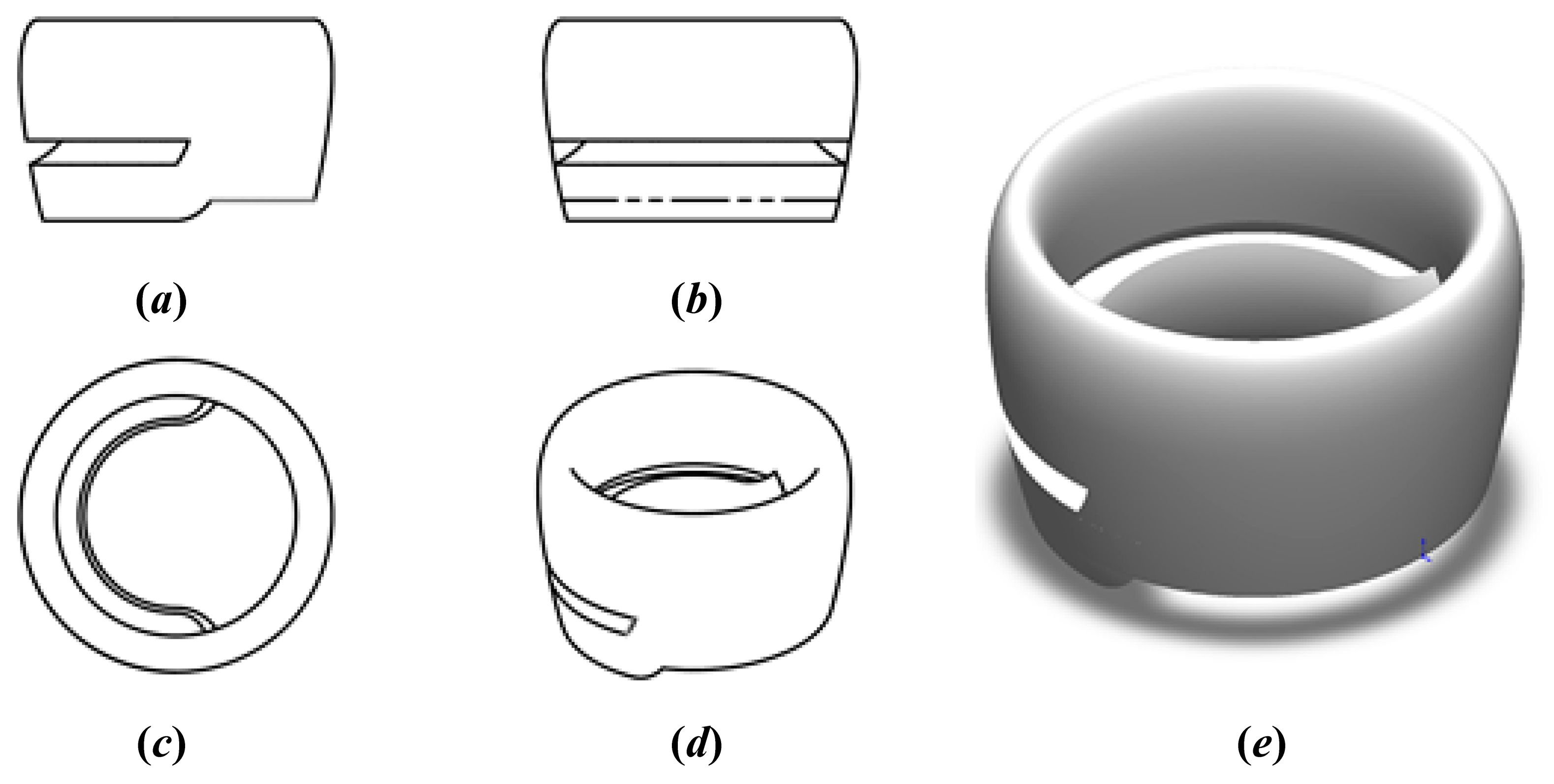
Structural views of the asymmetric duct and SolidWorks model. (a) Front view; (b) Left view; (c) Top view; (d) Isometric view; (e) SolidWorks model.
Figure 4.
Structural views of the asymmetric duct and SolidWorks model. (a) Front view; (b) Left view; (c) Top view; (d) Isometric view; (e) SolidWorks model.
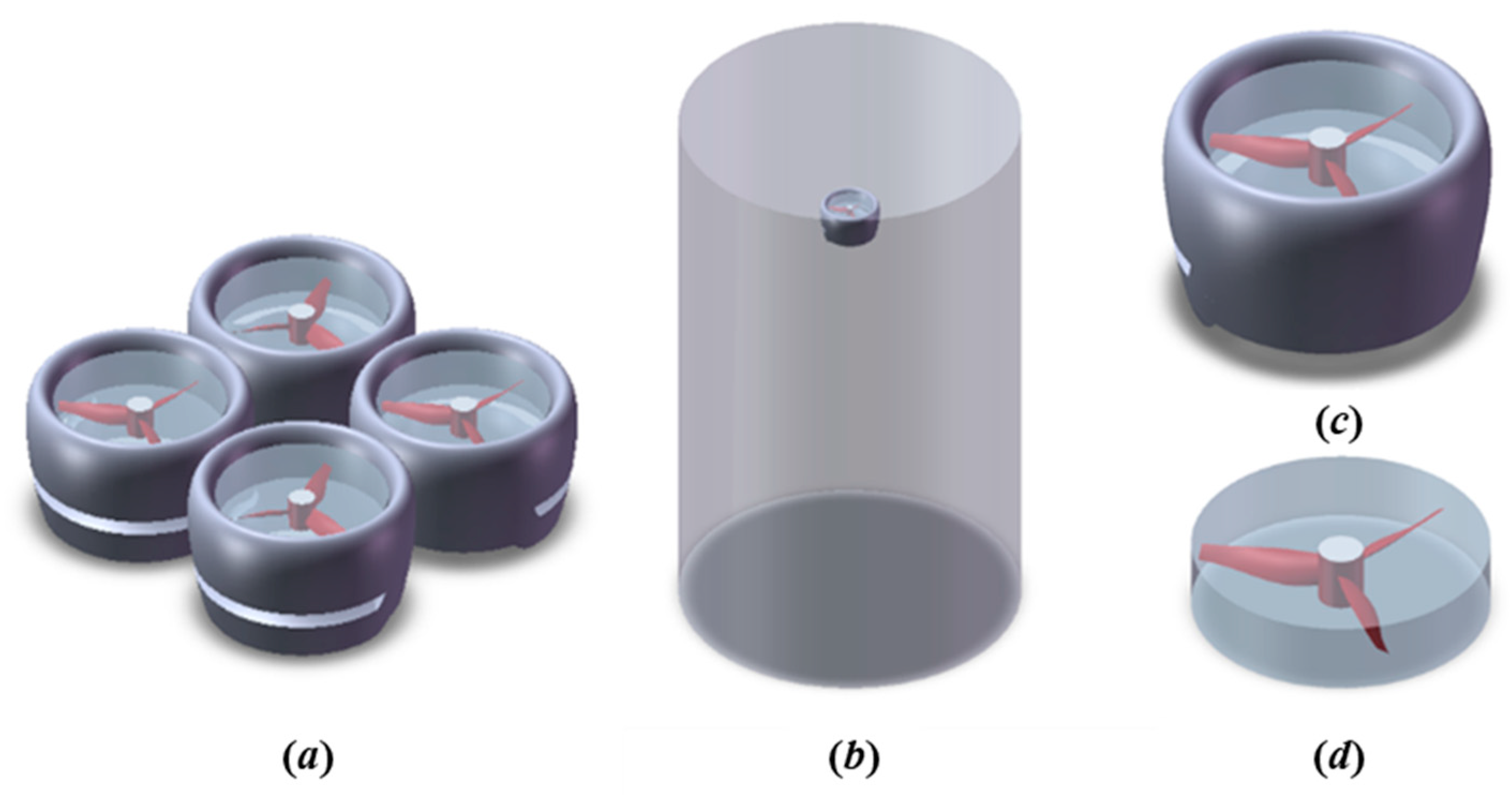
Figure 5.
Simulation model of the ducted UAV. (a) Overall model of the quadcopter; (b) outer flow field region; (c) computational model of a single duct; (d) rotation domain region.
Figure 5.
Simulation model of the ducted UAV. (a) Overall model of the quadcopter; (b) outer flow field region; (c) computational model of a single duct; (d) rotation domain region.
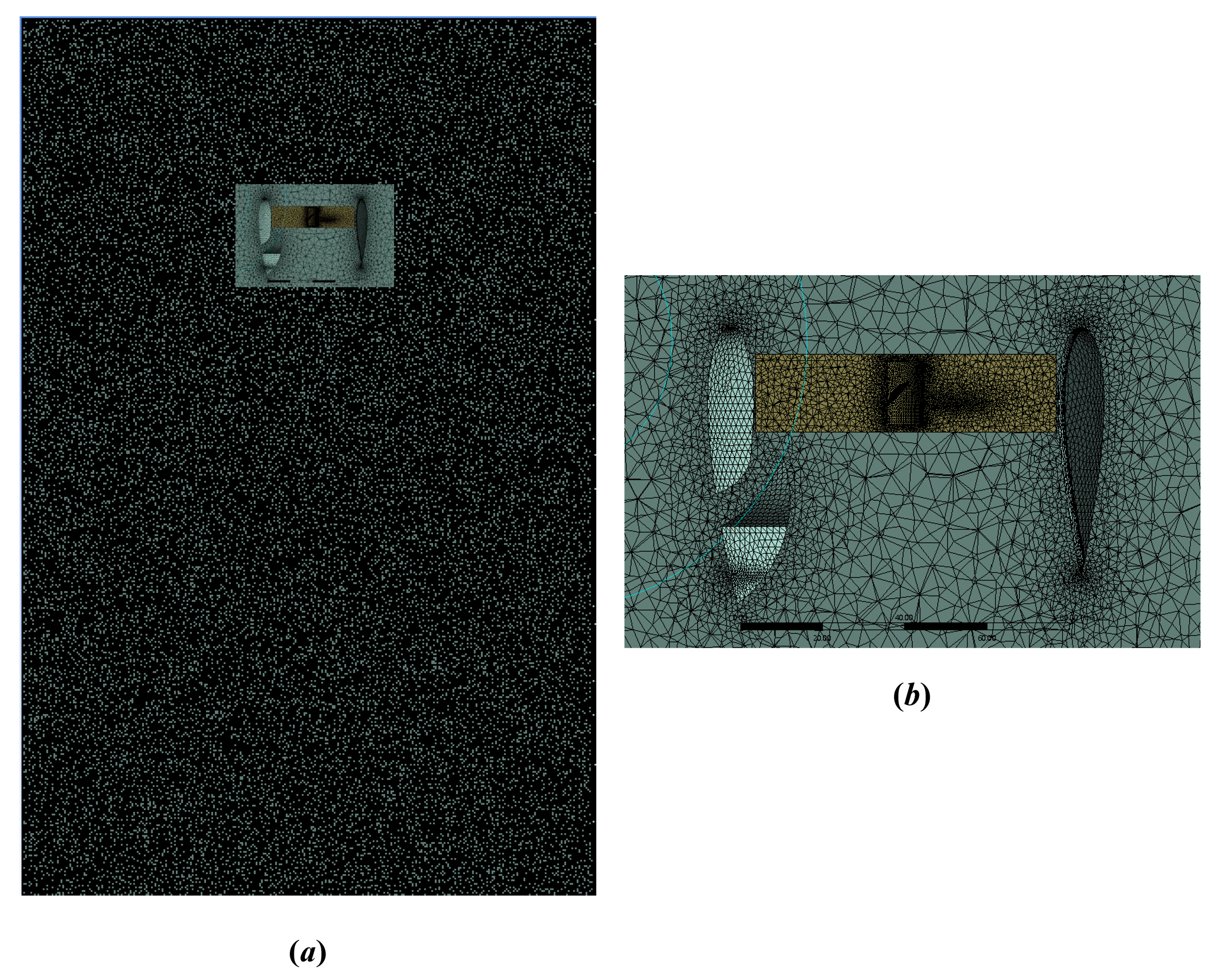
Figure 6.
Overall mesh and propeller region mesh. (a) Overall mesh; (b) Close-up of the propeller region.
Figure 6.
Overall mesh and propeller region mesh. (a) Overall mesh; (b) Close-up of the propeller region.
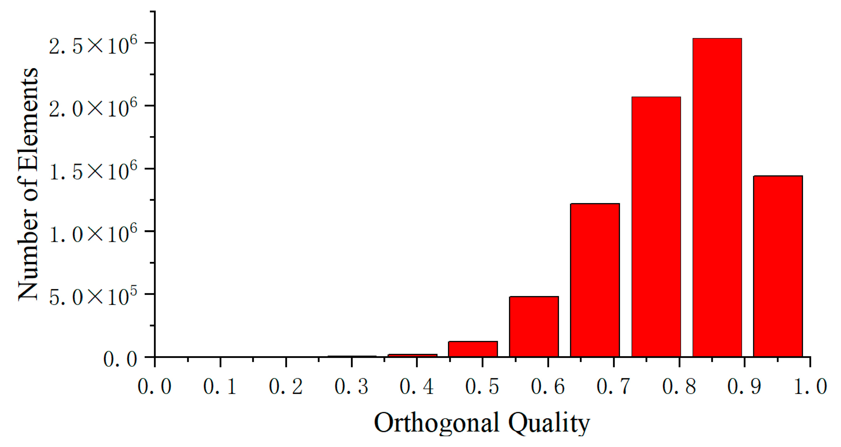
Figure 7.
Distribution of mesh counts under the Orthogonal Quality metric.
Figure 7.
Distribution of mesh counts under the Orthogonal Quality metric.
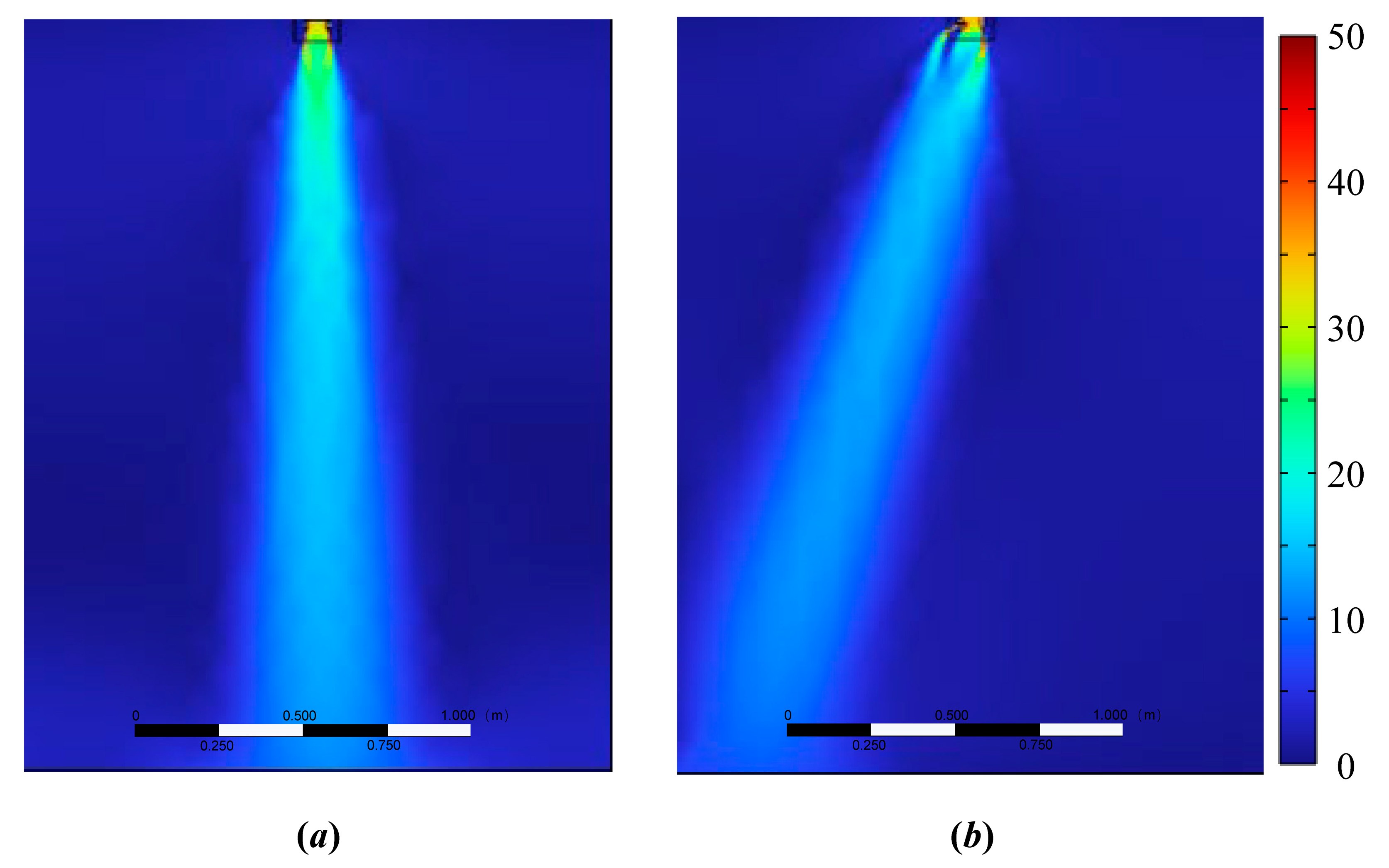
Figure 8.
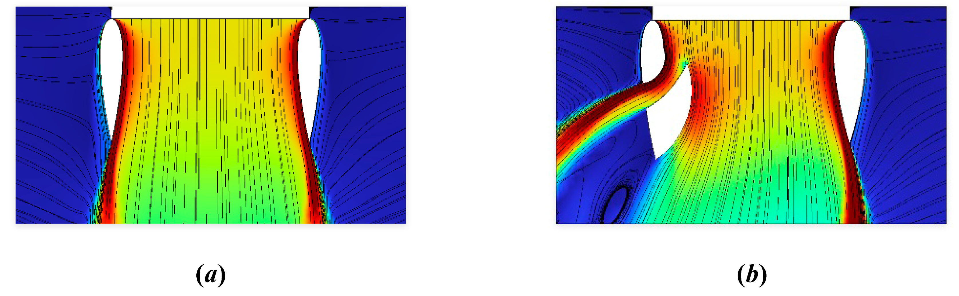
Comparison of external airflow velocity contours for the symmetric and asymmetric ducts. (a) Symmetric duct; (b) Asymmetric duct.
Figure 8.
Comparison of external airflow velocity contours for the symmetric and asymmetric ducts. (a) Symmetric duct; (b) Asymmetric duct.
Figure 9.
Comparison of streamlines for symmetric and asymmetric ducts. (a) Symmetric duct; (b) Asymmetric duct. Analysis of the characteristics of the internal velocity and pressure fields in asymmetric ducts.
Figure 9.
Comparison of streamlines for symmetric and asymmetric ducts. (a) Symmetric duct; (b) Asymmetric duct. Analysis of the characteristics of the internal velocity and pressure fields in asymmetric ducts.
Figure 10.
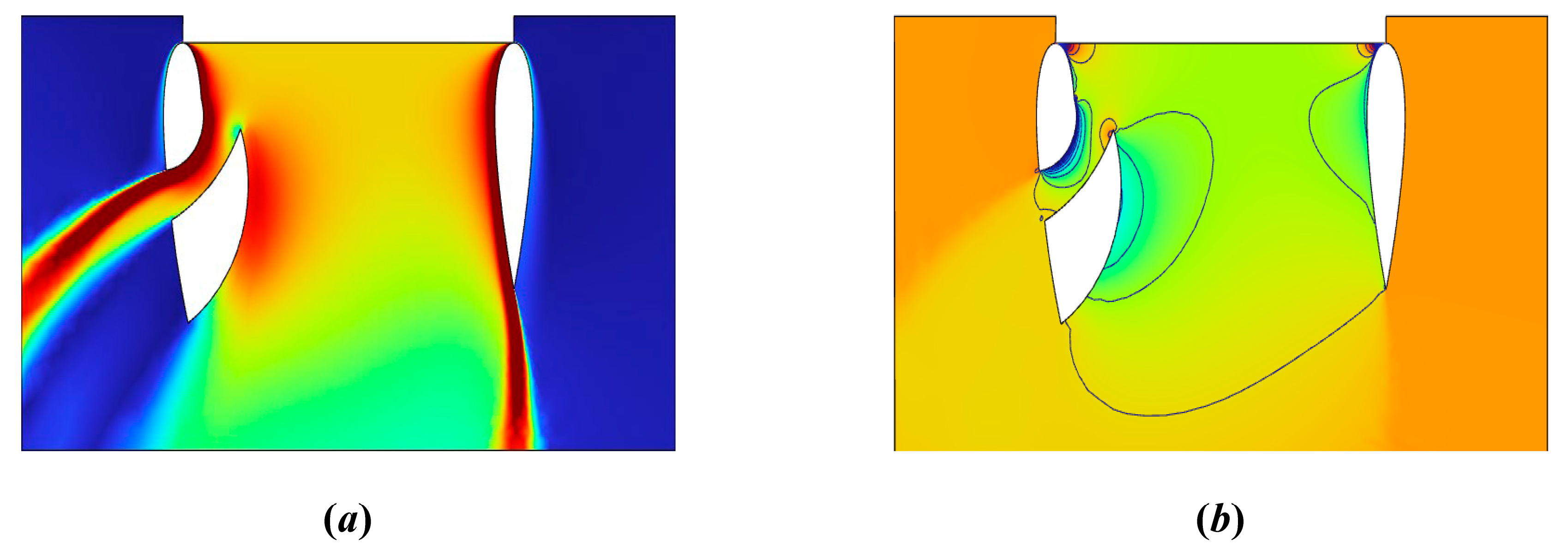
Internal velocity and pressure distributions in the duct under typical operating conditions. (a) Velocity contour plot; (b) Pressure contour plot.
Figure 10.
Internal velocity and pressure distributions in the duct under typical operating conditions. (a) Velocity contour plot; (b) Pressure contour plot.
Figure 11.
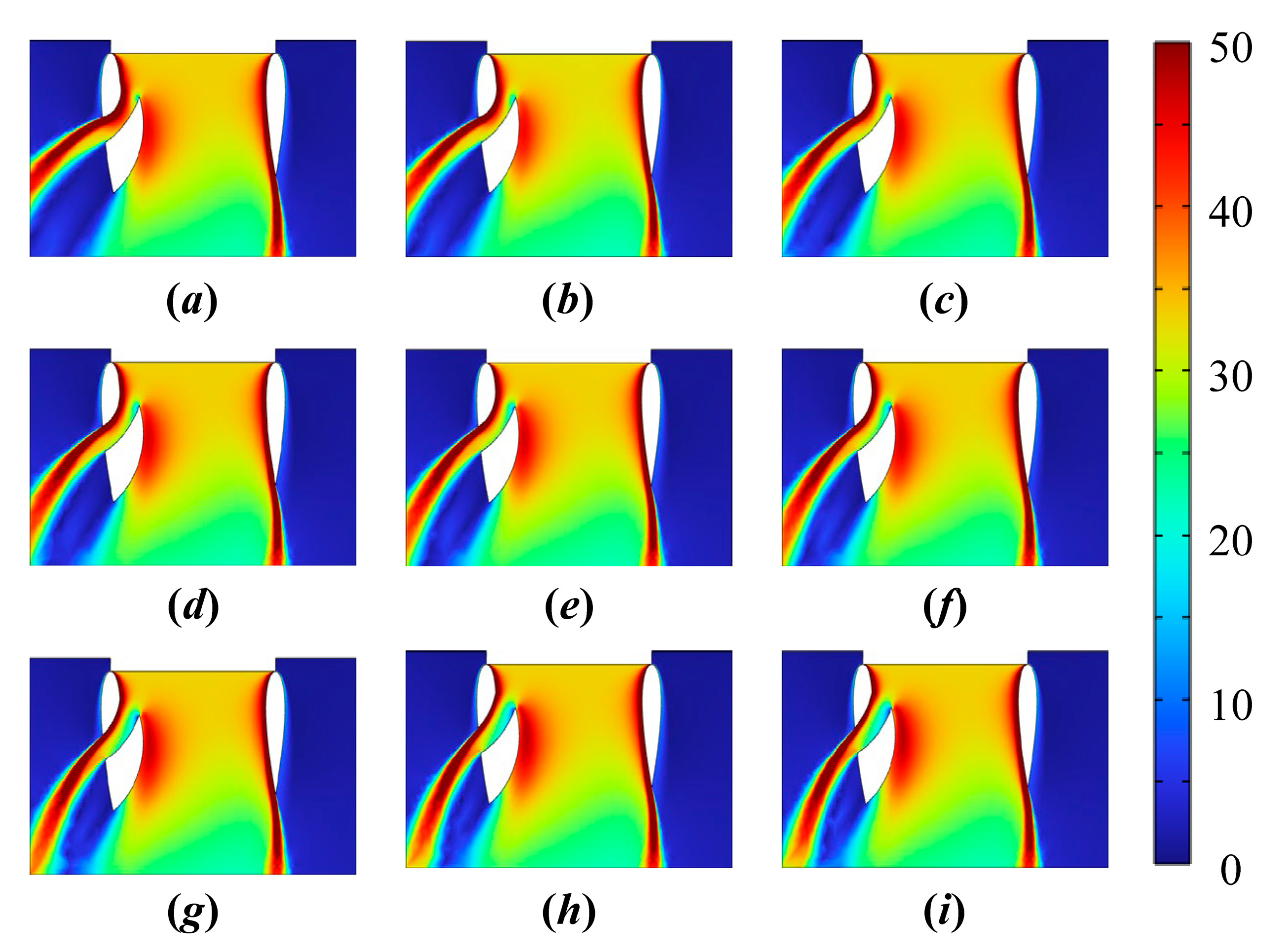
Velocity distribution inside the duct under different R1 conditions. (a–i) correspond to R1 = 10, 11, 12, 13, 14, 15, 20, 25, and 30 mm, respectively. The color scale indicates velocity magnitude (m·s−1).
Figure 11.
Velocity distribution inside the duct under different R1 conditions. (a–i) correspond to R1 = 10, 11, 12, 13, 14, 15, 20, 25, and 30 mm, respectively. The color scale indicates velocity magnitude (m·s−1).
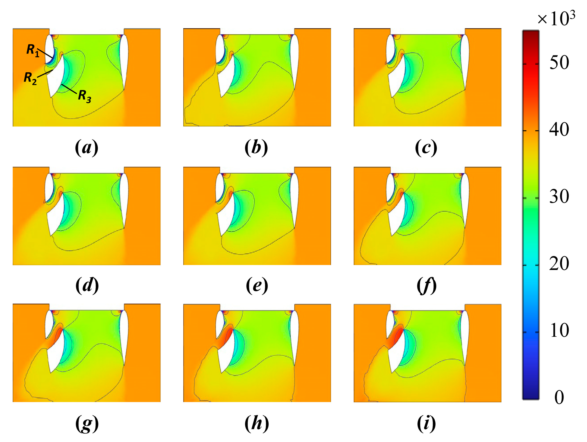
Figure 12.
Internal pressure distribution within the duct under different R1 conditions. (a–i) correspond to R1 = 10, 11, 12, 13, 14, 15, 20, 25, and 30 mm, respectively. The color scale indicates pressure magnitude (Pa).
Figure 12.
Internal pressure distribution within the duct under different R1 conditions. (a–i) correspond to R1 = 10, 11, 12, 13, 14, 15, 20, 25, and 30 mm, respectively. The color scale indicates pressure magnitude (Pa).
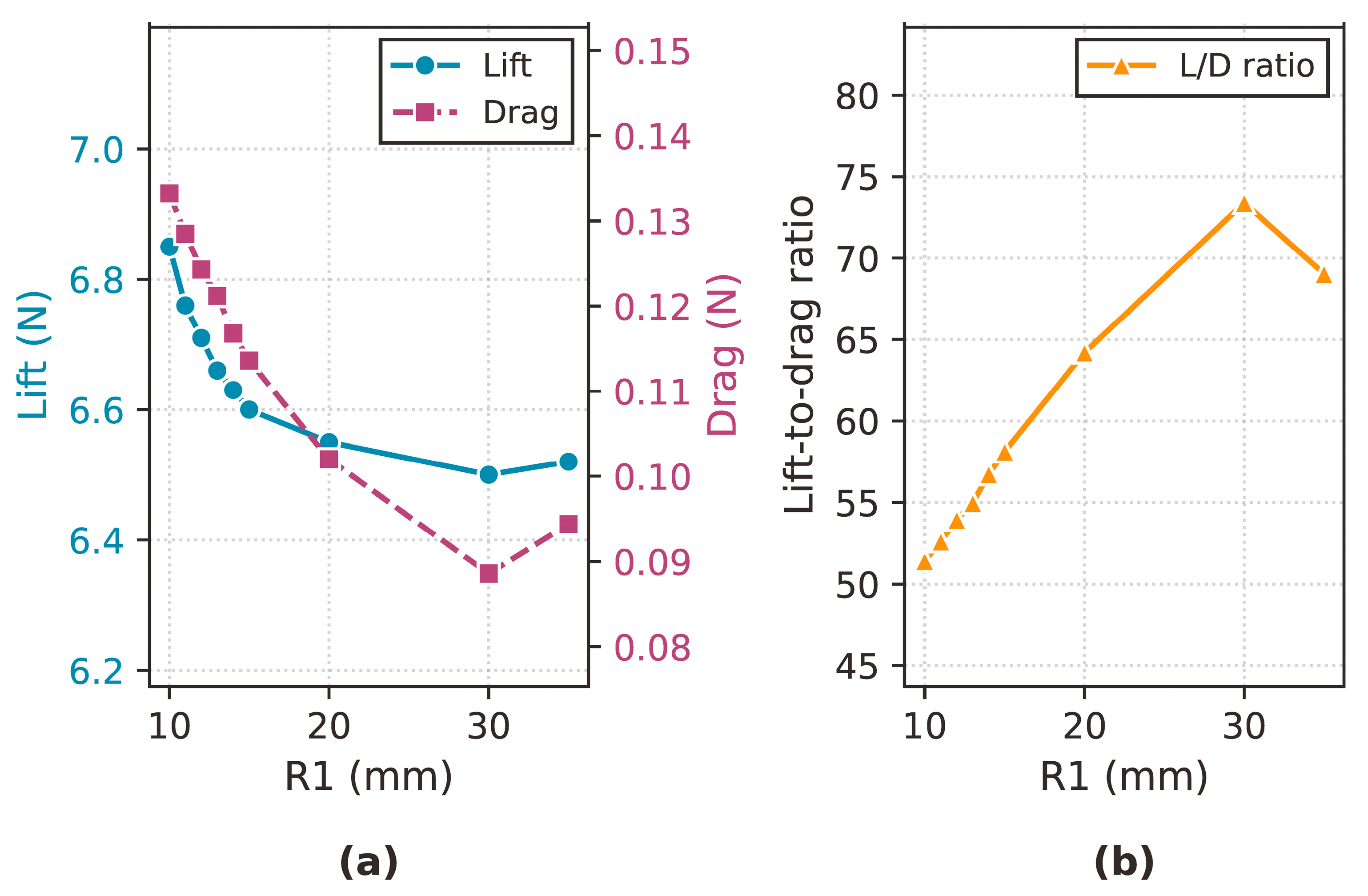
Figure 13.
Effects of R1 on lift, drag, and lift-to-drag ratio. (a) Lift and drag; (b) Lift-to-drag ratio.
Figure 13.
Effects of R1 on lift, drag, and lift-to-drag ratio. (a) Lift and drag; (b) Lift-to-drag ratio.
Figure 14.
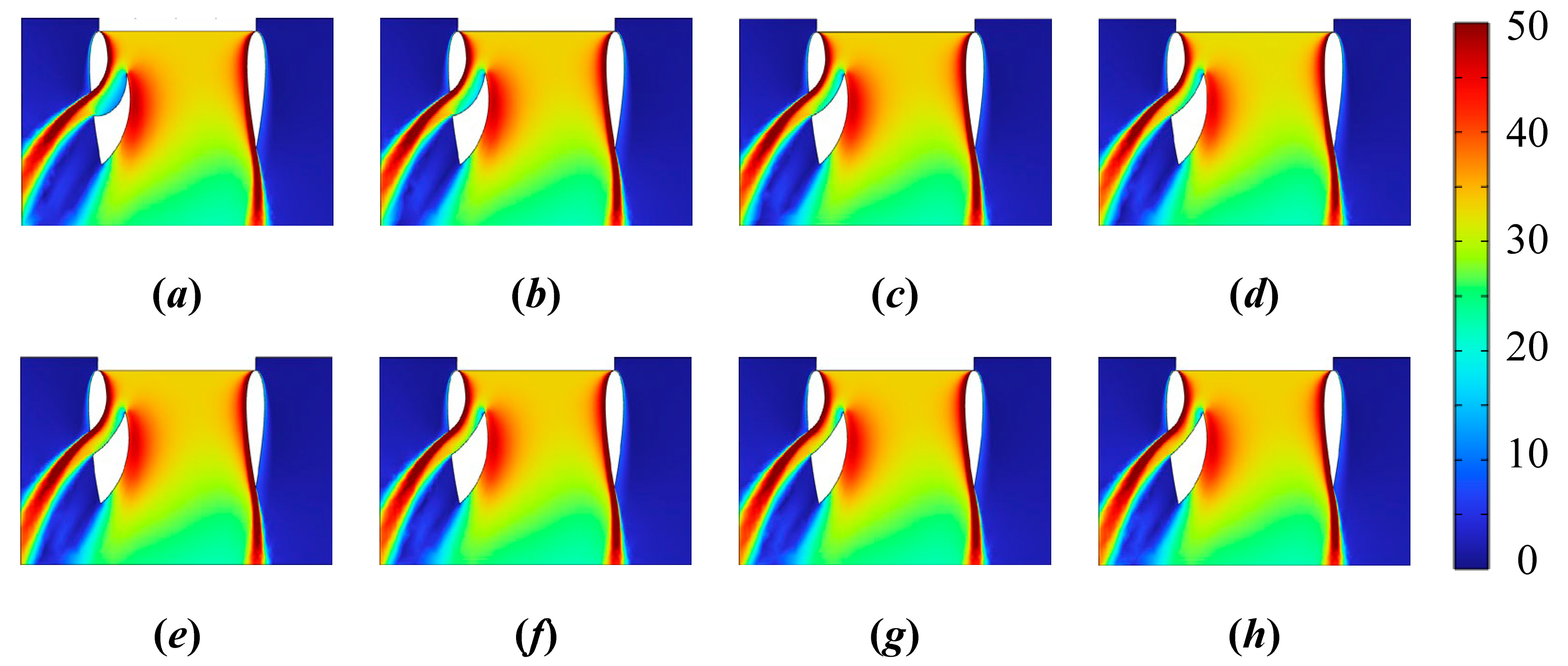
Velocity distribution inside the duct under different R2 conditions. (a–h) correspond to R2 = 15, 20, 25, 30, 35, 40, 45, and 50 mm, respectively. The color scale indicates velocity magnitude (m·s−1).
Figure 14.
Velocity distribution inside the duct under different R2 conditions. (a–h) correspond to R2 = 15, 20, 25, 30, 35, 40, 45, and 50 mm, respectively. The color scale indicates velocity magnitude (m·s−1).
Figure 15.
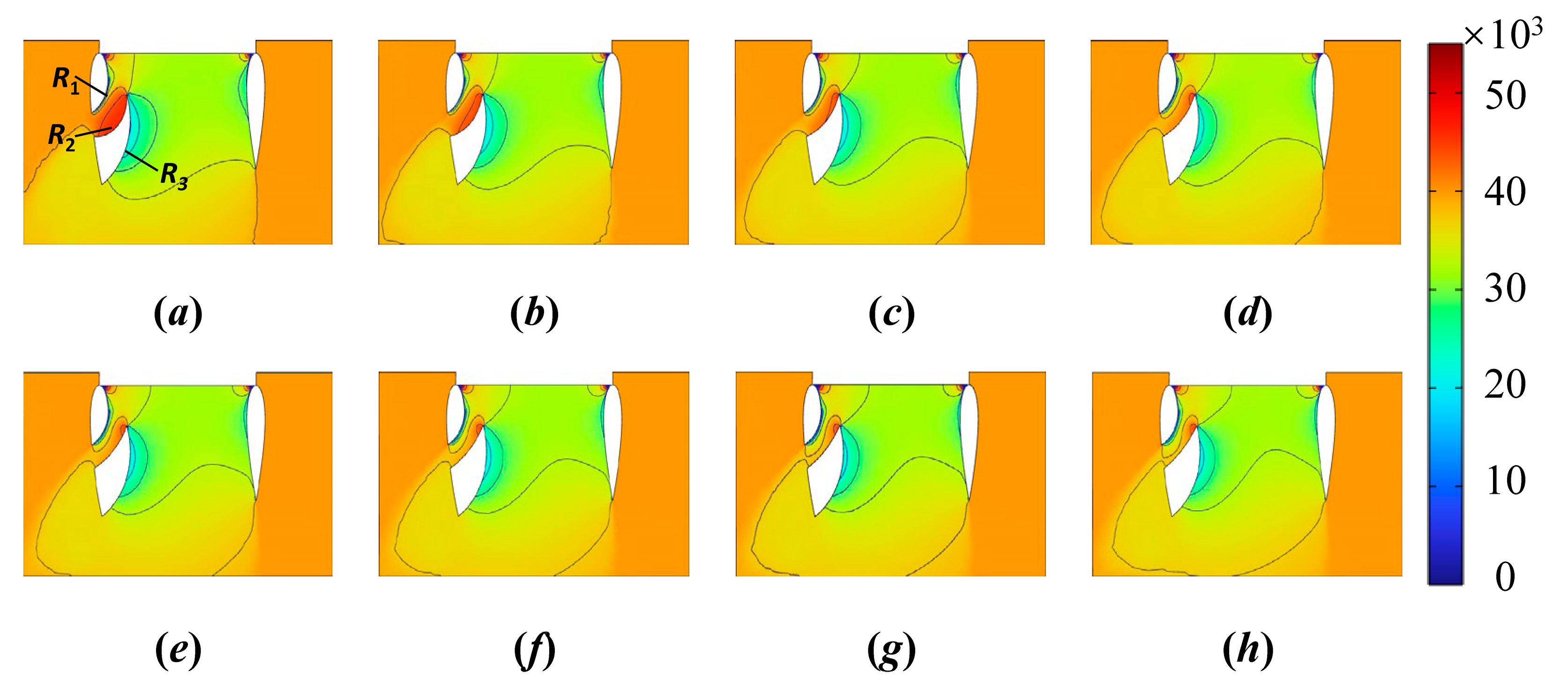
Internal pressure distribution in the duct under different R2 conditions. (a–h) correspond to R2 = 15, 20, 25, 30, 35, 40, 45, and 50 mm, respectively. The color scale indicates pressure magnitude (Pa).
Figure 15.
Internal pressure distribution in the duct under different R2 conditions. (a–h) correspond to R2 = 15, 20, 25, 30, 35, 40, 45, and 50 mm, respectively. The color scale indicates pressure magnitude (Pa).
Figure 16.
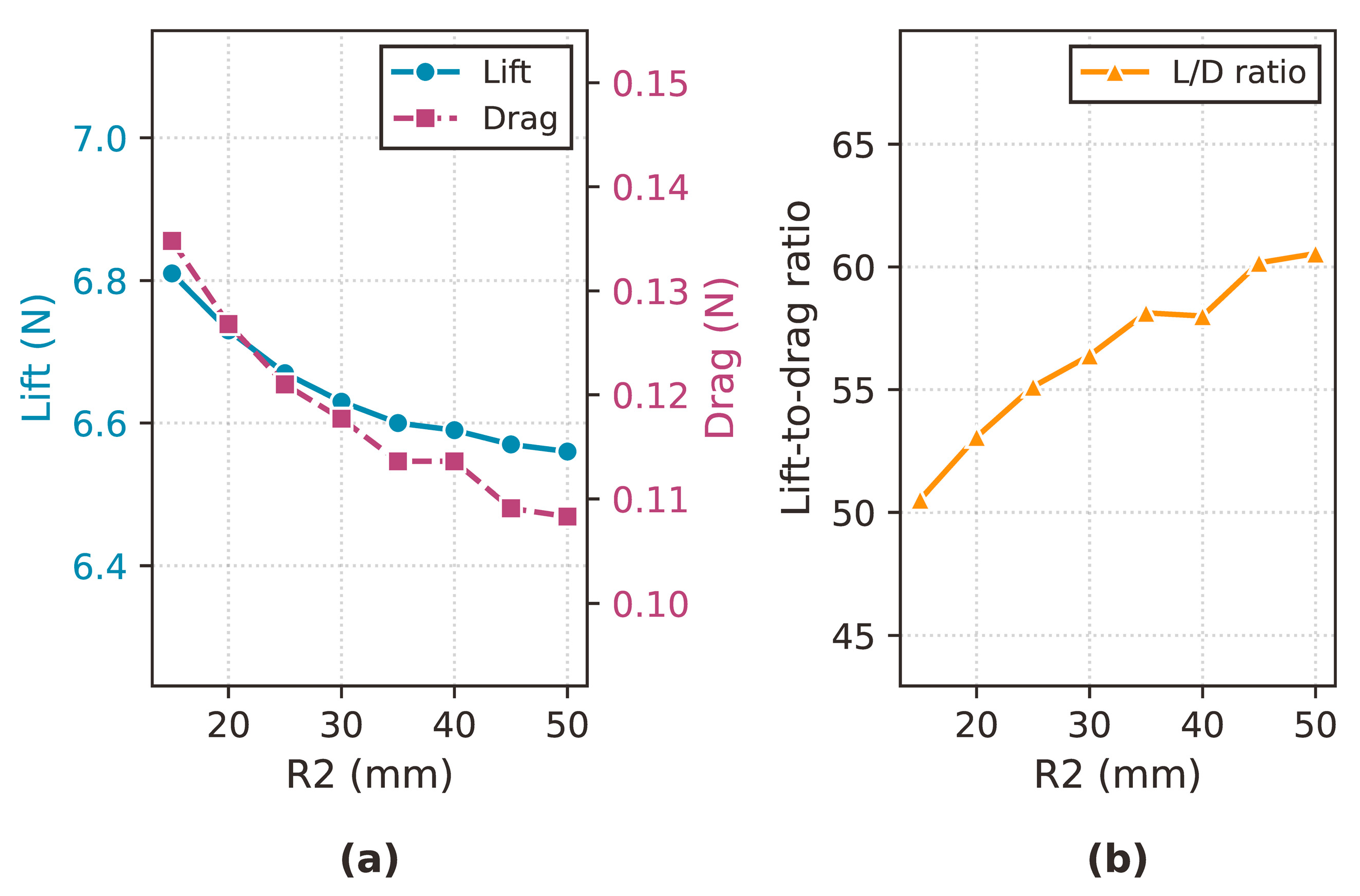
Effects of R2 on lift, drag, and lift-to-drag ratio. (a) Lift and drag; (b) Lift-to-drag ratio.
Figure 16.
Effects of R2 on lift, drag, and lift-to-drag ratio. (a) Lift and drag; (b) Lift-to-drag ratio.
Figure 17.
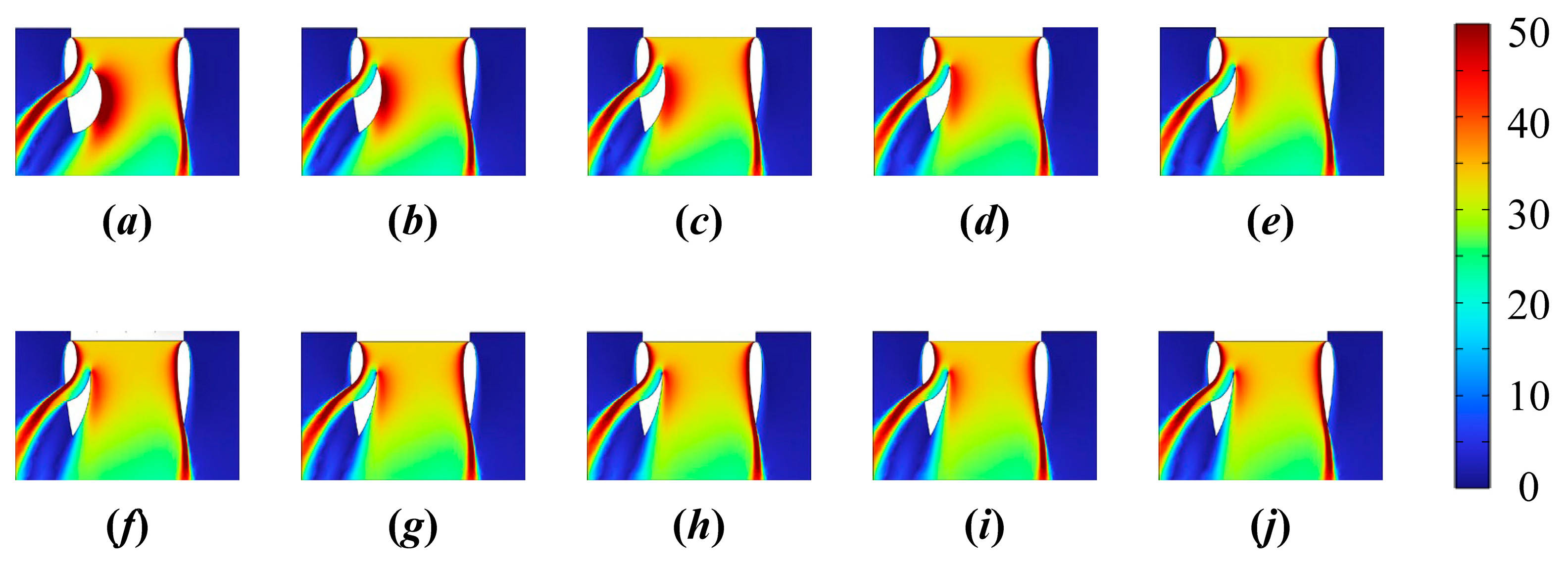
Velocity distribution inside the duct under different R3 conditions. (a–j) correspond to R3 = 20, 25, 30, 35, 40, 45, 50, 55, 60, and 65 mm, respectively. The color scale indicates velocity magnitude (m·s−1).
Figure 17.
Velocity distribution inside the duct under different R3 conditions. (a–j) correspond to R3 = 20, 25, 30, 35, 40, 45, 50, 55, 60, and 65 mm, respectively. The color scale indicates velocity magnitude (m·s−1).
Figure 18.
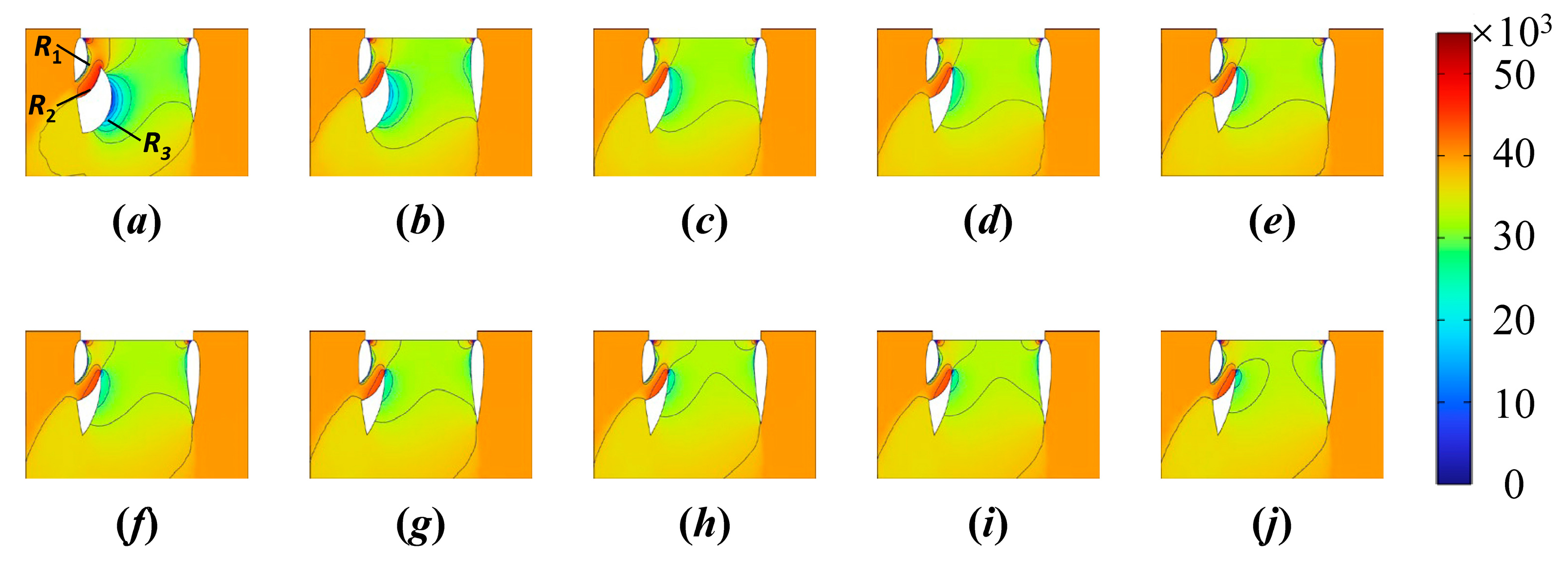
Internal pressure distribution in the duct under different R3 conditions. (a–j) correspond to R3 = 20, 25, 30, 35, 40, 45, 50, 55, 60, and 65 mm, respectively. The color scale indicates pressure magnitude (Pa).
Figure 18.
Internal pressure distribution in the duct under different R3 conditions. (a–j) correspond to R3 = 20, 25, 30, 35, 40, 45, 50, 55, 60, and 65 mm, respectively. The color scale indicates pressure magnitude (Pa).
Figure 19.
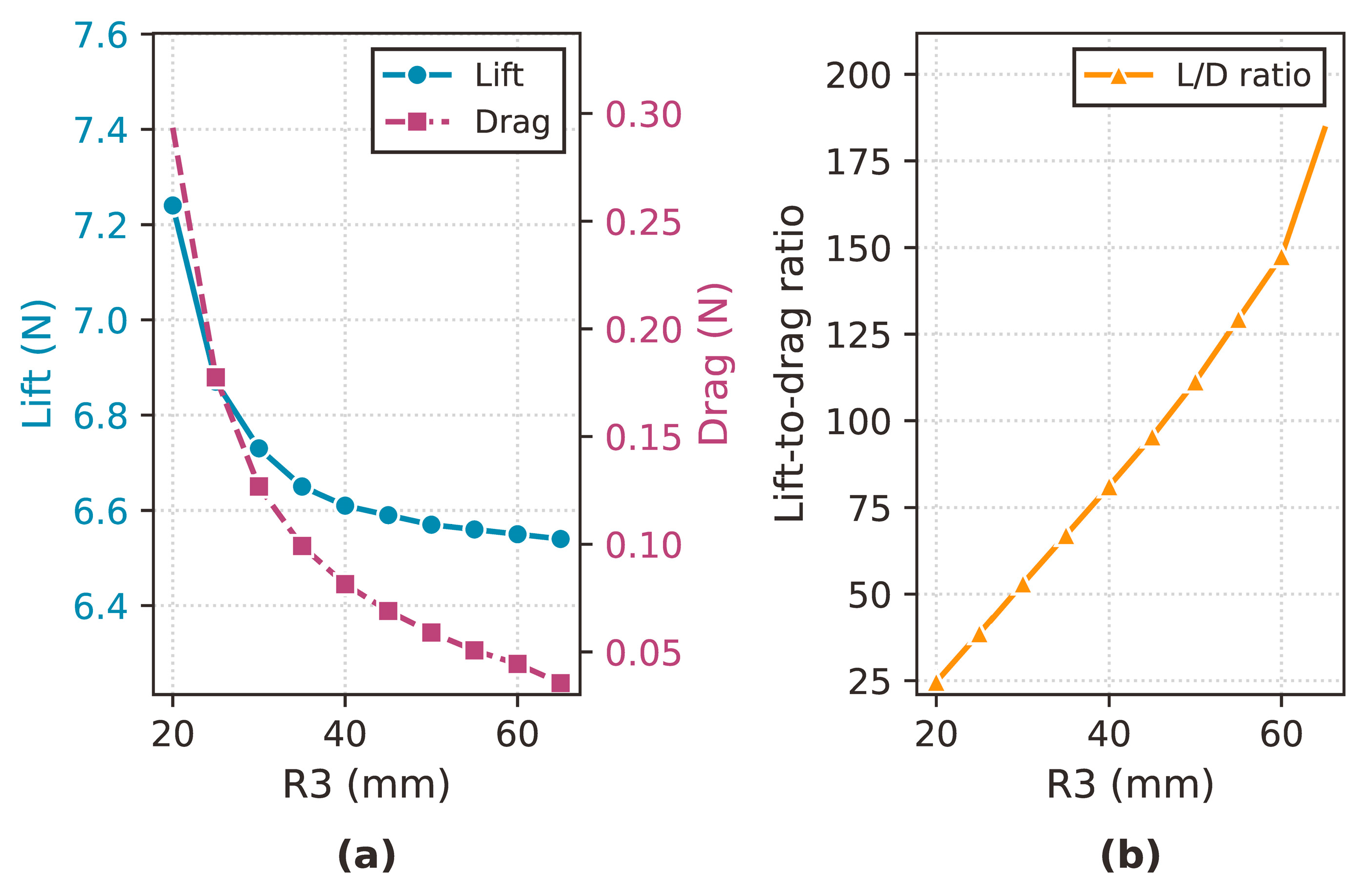
Effects of R3 on lift, drag, and lift-to-drag ratio. (a) Lift and drag; (b) Lift-to-drag ratio.
Figure 19.
Effects of R3 on lift, drag, and lift-to-drag ratio. (a) Lift and drag; (b) Lift-to-drag ratio.
Figure 20.
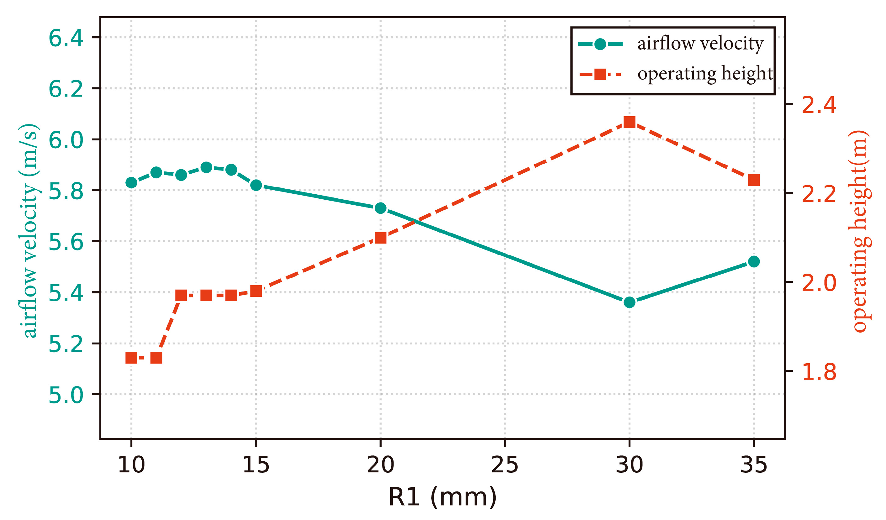
Curves showing the effect of R1 on airflow velocity and UAV operating height in the pollination area.
Figure 20.
Curves showing the effect of R1 on airflow velocity and UAV operating height in the pollination area.
Figure 21.
External airflow distributions under different R1 conditions. (a–i) correspond to R1 = 10, 11, 12, 13, 14, 15, 20, 25, and 30 mm, respectively.
Figure 21.
External airflow distributions under different R1 conditions. (a–i) correspond to R1 = 10, 11, 12, 13, 14, 15, 20, 25, and 30 mm, respectively.
Figure 22.
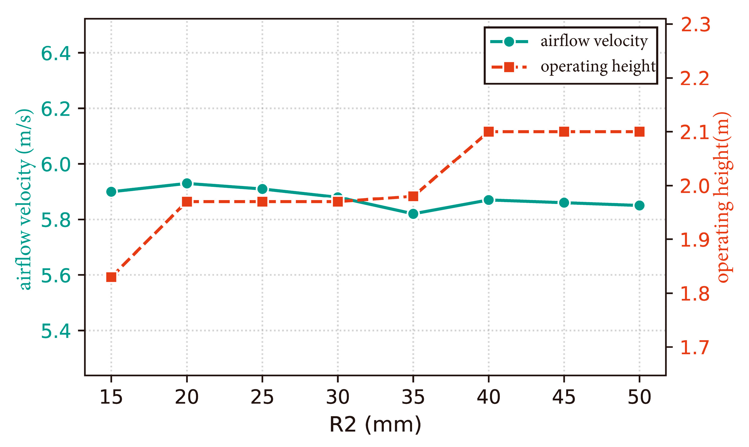
Curves showing the effect of R2 on airflow velocity and UAV operating height in the pollination zone.
Figure 22.
Curves showing the effect of R2 on airflow velocity and UAV operating height in the pollination zone.
Figure 23.
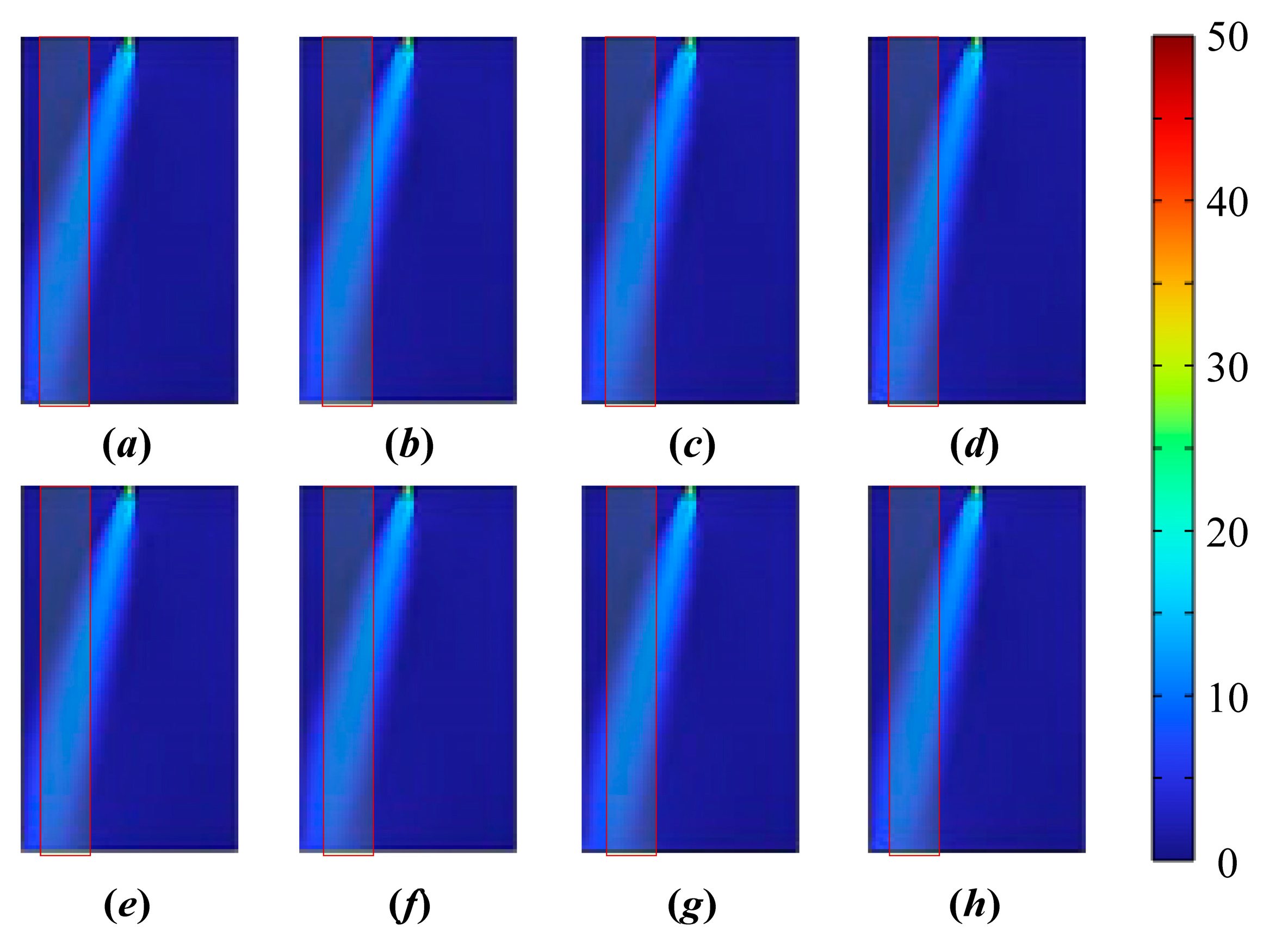
Distribution of external downwash flow fields under different R2 conditions. (a–h) correspond to R2 = 15, 20, 25, 30, 35, 40, 45, and 50 mm, respectively.
Figure 23.
Distribution of external downwash flow fields under different R2 conditions. (a–h) correspond to R2 = 15, 20, 25, 30, 35, 40, 45, and 50 mm, respectively.
Figure 24.
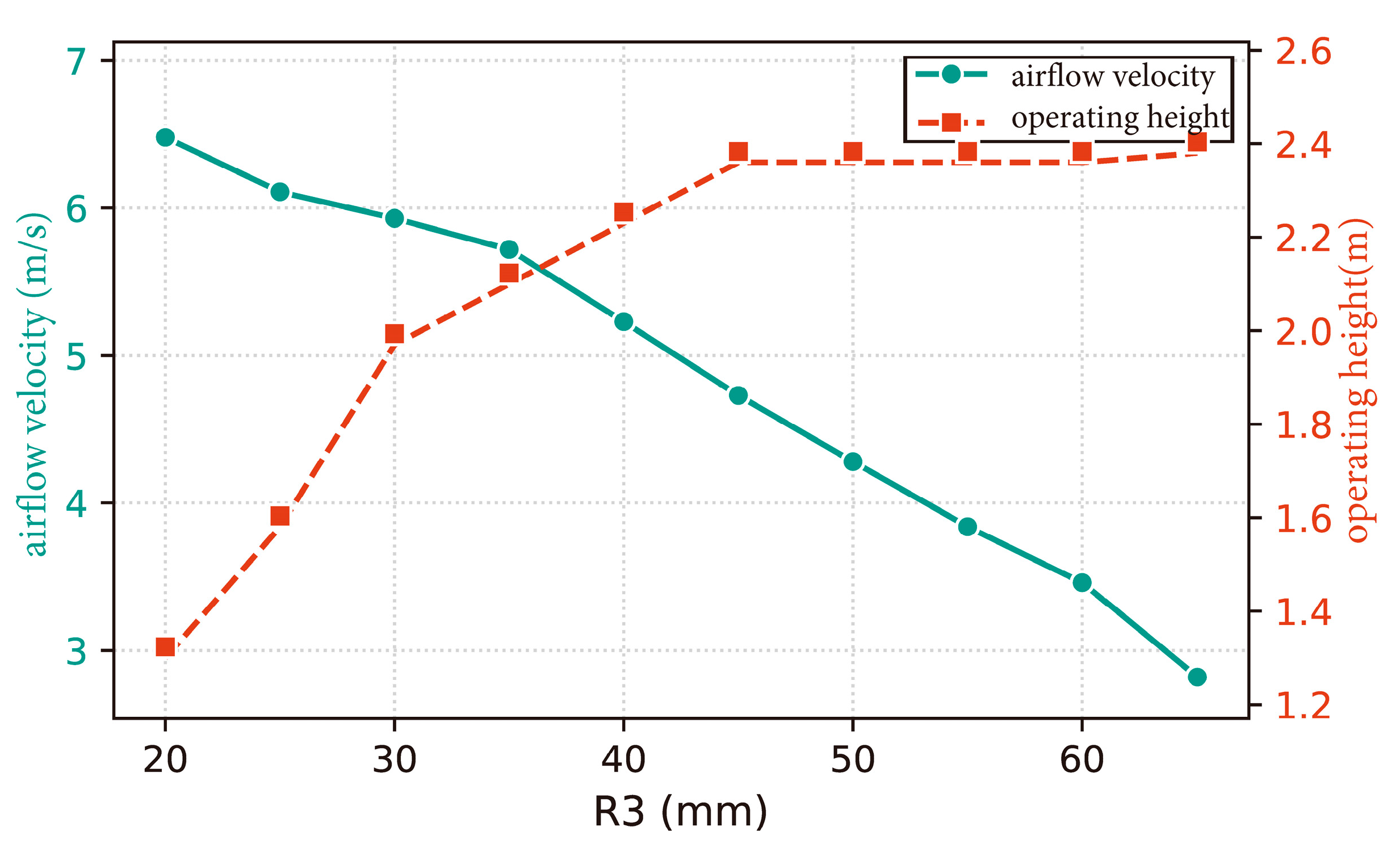
Effects of R3 on airflow velocity within the pollination region and UAV operating height.
Figure 24.
Effects of R3 on airflow velocity within the pollination region and UAV operating height.
Figure 25.
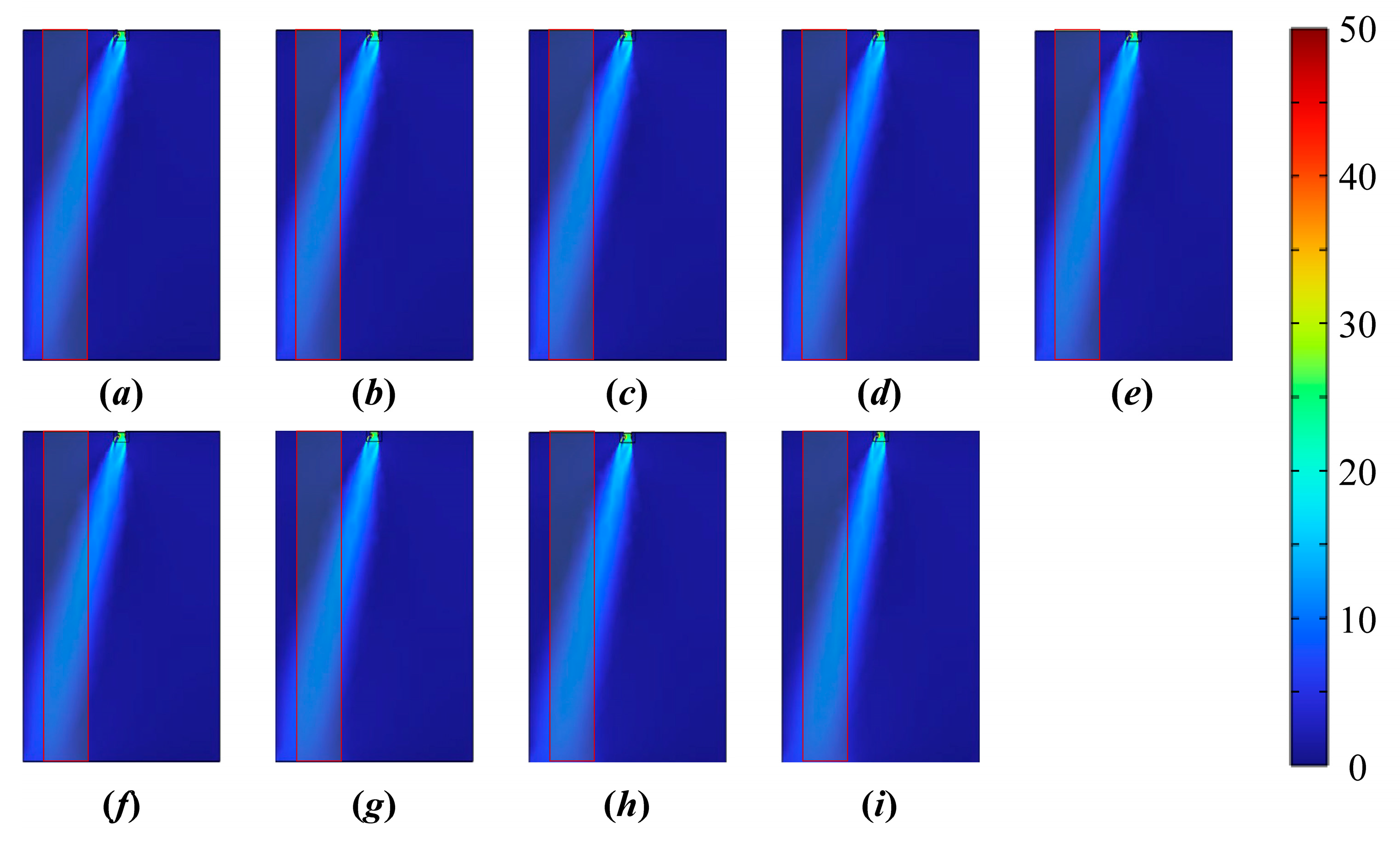
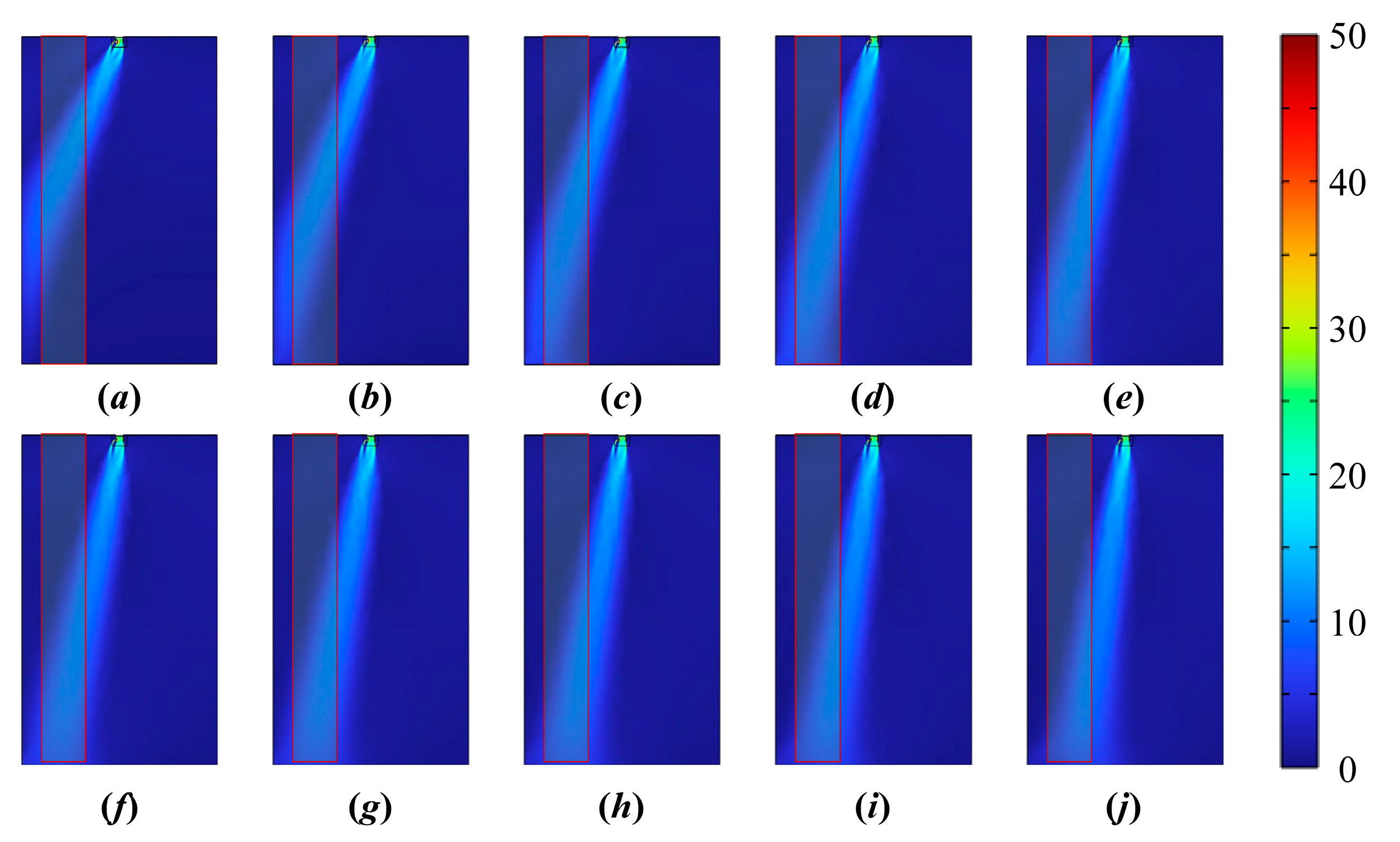
External airflow distributions under different R3 conditions. (a–j) correspond to R3 = 20, 25, 30, 35, 40, 45, 50, 55, 60, and 65 mm, respectively.
Figure 25.
External airflow distributions under different R3 conditions. (a–j) correspond to R3 = 20, 25, 30, 35, 40, 45, 50, 55, 60, and 65 mm, respectively.
Figure 26.
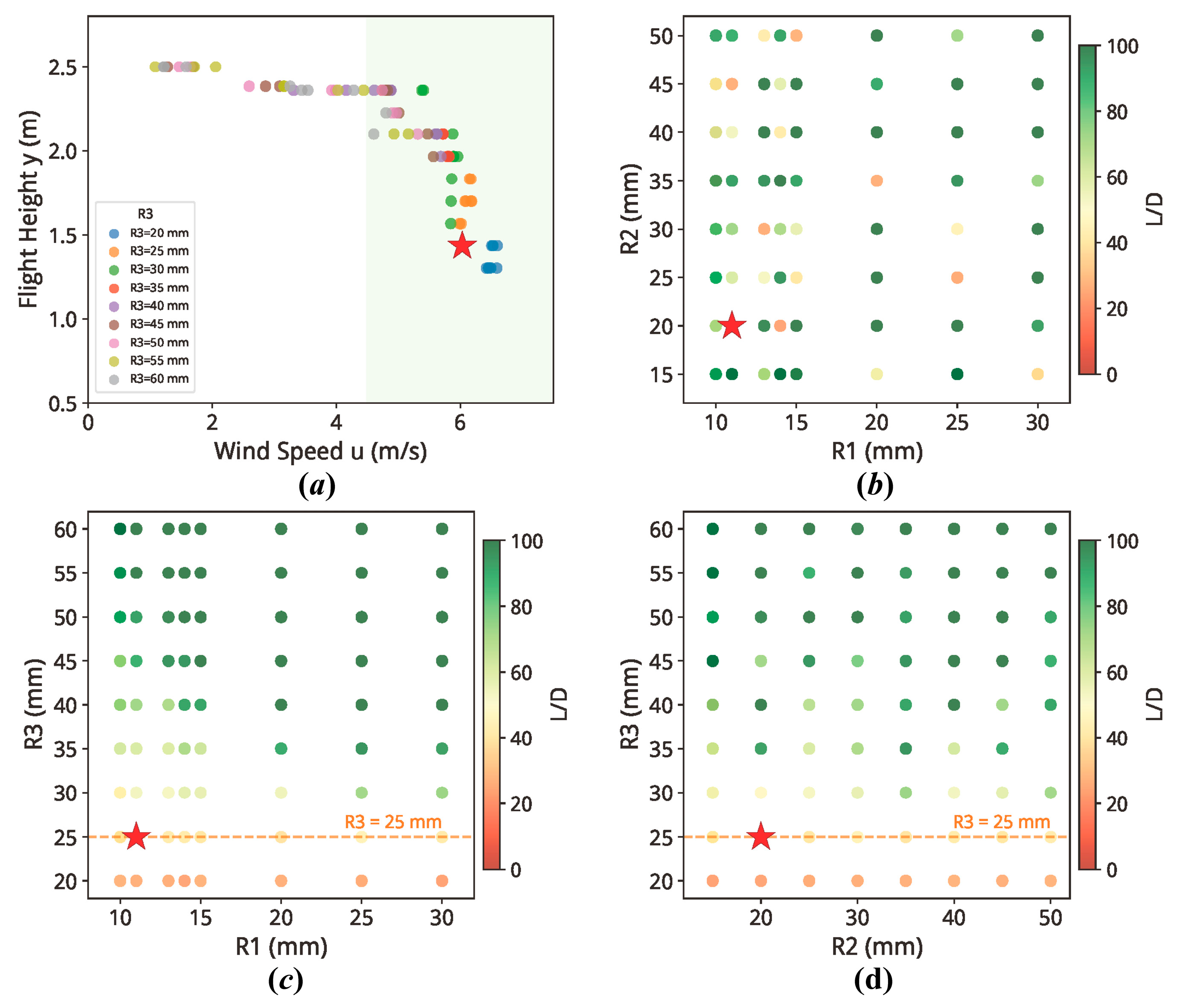
Parameter-space distribution of the orthogonal experiment. (a) Airflow velocity within the pollination region versus UAV operating height, color-coded by R3; (b) R1–R2, (c) R1–R3, and (d) R2–R3 projections, with lift-to-drag ratio (L/D) represented by the color scale. The red star indicates the selected configuration (R1 = 11 mm, R2 = 20 mm, and R3 = 25 mm). The green shaded region in (a) denotes u > 4.5 m·s−1, and the dashed orange line in (c,d) indicates R3 = 25 mm.
Figure 26.
Parameter-space distribution of the orthogonal experiment. (a) Airflow velocity within the pollination region versus UAV operating height, color-coded by R3; (b) R1–R2, (c) R1–R3, and (d) R2–R3 projections, with lift-to-drag ratio (L/D) represented by the color scale. The red star indicates the selected configuration (R1 = 11 mm, R2 = 20 mm, and R3 = 25 mm). The green shaded region in (a) denotes u > 4.5 m·s−1, and the dashed orange line in (c,d) indicates R3 = 25 mm.
Table 1.
Geometric parameters of the asymmetric duct.
Table 1.
Geometric parameters of the asymmetric duct.
| Item | Value (mm) | Item | Value (mm) |
|---|
| d1 | 92 | h1 | 10 |
| d2 | 80 | h2 | 31.5 |
| d3 | 72 | h3 | 68 |
| | | h4 | 60 |
Table 2.
Grid independence verification results.
Table 2.
Grid independence verification results.
| Grid | Total Elements | Velocity at 0.5 m (m·s−1) | Velocity at 1.0 m (m·s−1) | Relative Error (%) |
|---|
| Mesh-1 | 2,456,789 | 6.21 | 3.87 | 9.1/4.9 |
| Mesh-2 | 7,892,153 | 6.72 | 4.02 | 1.6/1.2 |
| Mesh-3 | 15,678,234 | 6.83 | 4.07 | — |
Table 3.
Comparison results of CFD and experimental wind speeds.
Table 3.
Comparison results of CFD and experimental wind speeds.
| Location/m | Value 1/(m·s−1) | Value 2/(m·s−1) | Value 3/(m·s−1) | Experimental Mean/(m·s−1) | CFD Result/(m·s−1) | Absolute
Error/(m·s−1) | Relative Error/% |
|---|
| 0.5 | 5.84 | 5.88 | 5.56 | 5.76 | 6.50 | 0.74 | 12.85 |
| 1 | 4.13 | 4.04 | 3.90 | 4.02 | 4.06 | 0.04 | 1.0 |
Table 4.
Factors and levels for the quasi-orthogonal parameter combination design.
Table 4.
Factors and levels for the quasi-orthogonal parameter combination design.
| Level | R1 (mm) | R2 (mm) | R3 (mm) |
|---|
| 1 | 10 | 15 | 20 |
| 2 | 11 | 20 | 25 |
| 3 | 13 | 25 | 30 |
| 4 | 14 | 30 | 35 |
| 5 | 15 | 35 | 40 |
| 6 | 20 | 40 | 45 |
| 7 | 25 | 45 | 50 |
| 8 | 30 | 50 | 55 |
| 9 | — | — | 60 |
Table 5.
Representative Parameter Combinations Satisfying the adopted airflow and operating-height criteria at R3 = 25 mm.
Table 5.
Representative Parameter Combinations Satisfying the adopted airflow and operating-height criteria at R3 = 25 mm.
| No. | R1/mm | R2/mm | R3/mm | Wind Speed in Pollination Area/(m·s−1) | UAV Operating Height/m | Lift/N | Drag/N | Lift-to-Drag Ratio |
|---|
| 1 | 11 | 20 | 25 | 6.032 | 1.435 | 7.037 | 0.190 | 37.0 |
| 2 | 25 | 30 | 25 | 6.148 | 1.834 | 6.674 | 0.150 | 44.6 |
| 3 | 30 | 15 | 25 | 6.173 | 1.833 | 6.811 | 0.165 | 41.3 |
| 4 | 15 | 25 | 25 | 6.185 | 1.701 | 6.810 | 0.171 | 39.9 |
| 5 | 13 | 50 | 25 | 6.094 | 1.701 | 6.741 | 0.161 | 42.0 |
| 6 | 10 | 45 | 25 | 5.989 | 1.568 | 6.928 | 0.173 | 40.0 |