Spatiotemporal Evolution Characteristics of Cropland Use Stability in Guangdong Province, China and Its Implications for Cropland Management

Abstract

Cropland use stability is vital for sustaining the productive and ecological functions of cropland. Existing multidimensional assessment frameworks rarely distinguish between quantity change and spatial change, nor do they examine their interactions across hierarchical scales. Using annual 30 m land cover data for Guangdong Province, China (1990–2024), this study developed a two-dimensional stability framework integrating quantity and spatial indicators, using a pixel-tracking strategy applied within each five-year interval to capture interannual dynamics. Analyses were conducted at provincial, agricultural zone, and city scales. Results showed that provincial stability exhibited a fluctuating upward trajectory, with the lowest point in 2005–2009. Regional patterns diverged markedly, and city-level stability exhibited spatial heterogeneity, with pronounced disparities between high- and low-stability cities. Grade transition and quadrant analyses further revealed that quantity and spatial stability do not always move in tandem, and single-dimension assessments may provide an incomplete picture of cropland use stability. These findings suggest that incorporating both dimensions into monitoring frameworks could support more differentiated cropland management strategies.

1. Introduction

Cropland serves as the foundation of food production and a critical guarantee of national food security and sustainable agricultural development [1,2,3]. However, under the combined pressures of industrialization, rapid urbanization, and climate change, cropland resources face increasing threats from quantity loss, quality degradation, and ecological decline [4,5,6,7,8]. In this context, cropland use stability—defined as the capacity of cropland to sustainably maintain its productive and ecological functions—has gained growing attention from both researchers and policymakers [9,10,11,12]. Nevertheless, the scientific definition and systematic assessment of cropland use stability require further investigation.

A unified definition of cropland stability has yet to emerge in the literature [13]. The concept can be traced back to the attention given to unstable cropland in China’s national land survey practice. The Bulletin of the Second National Land Survey classified several categories of cropland as “unstable”—including land within forests, grasslands, or flood control zones, as well as land affected by desertification and other degradation factors. Such cropland undermines protection effectiveness and poses a risk to national food security. Despite this recognition, systematic research on the status, assessment, and management of such cropland has long been insufficient [14,15,16,17]. Related studies have primarily focused on current land use status and property rights [18,19,20,21]. While these efforts provide a basis for differentiated management strategies, they tend to emphasize the identification of unstable conditions rather than the continuity of cropland use over time.

More recently, research has shifted toward cropland under long-term stable use, examining optimal crop growth environments and farmland management practices [22,23]. As understanding of cropland systems has deepened, multidimensional assessment frameworks have emerged, marking a transition from static descriptions to dynamic analysis of cropland stability [24,25]. Some studies integrate quantity, quality, and spatial patterns indicators from land-use and landscape perspectives [26,27,28,29], while others adopt an ecosystem service lens, emphasizing the capacity of cropland to sustain the provision of goods and services [30,31,32].

Despite notable progress, two significant research gaps remain. First, existing frameworks typically aggregate indicators across dimensions into a composite index, without distinguishing between quantity stability and spatial stability—two distinct aspects of cropland change. Quantity stability reflects the retention and fluctuation of cropland area, whereas spatial stability captures the locational persistence and pattern integrity of cropland patches. These dimensions may differ substantially in their evolution trajectories and policy implications. For instance, cropland quantity may remain stable at the aggregate level, while substantial spatial displacement could occur through the occupation of high-quality land and compensation with marginal land. This practice maintains area statistics on paper but undermines actual food production capacity. However, the coupling and divergence between the two dimensions have not yet been adequately explored. Second, most empirical studies are confined to a single administrative scale. This overlooks the scale-dependent nature of stability dynamics and limits their applicability to multi-scale, differentiated management.

To address these gaps, this study develops a two-dimensional cropland use stability assessment framework. The framework explicitly distinguishes quantity and spatial stability, and it examines their spatiotemporal evolution characteristics across multiple scales using long-term remote sensing data. Specifically, indicators are selected from the two dimensions for independent assessment and coupled analysis, thereby disentangling their differences and interrelationships during the evolution process. A key novelty of this framework is that it explicitly decouples quantity from spatial stability. This stands in contrast to conventional frameworks, which aggregate multiple dimensions into a single composite index and may thus mask divergent trajectories—such as maintaining area statistics through spatial displacement. Furthermore, the framework applies annual pixel tracking within fixed intervals rather than comparing only endpoints. This allows it to capture interannual fluctuations and temporary disturbances that endpoint-based comparisons tend to smooth over. This decoupling could provide a diagnostic layer for distinguishing whether stability changes originate from area loss or configurational fragmentation, offering clearer management signals for permanent basic farmland protection and urban sprawl control.

Guangdong Province is chosen as the study area. As a frontier region of China’s reform and opening-up, and one of the most rapidly urbanizing provinces in the country, Guangdong faces particularly acute conflicts between cropland protection and construction land expansion, making it a representative case for validating the effectiveness of such a two-dimensional assessment framework [33]. Nested comparisons are conducted at three scales—the entire province, the four major agricultural functional zones, and the 21 prefecture-level cities—to systematically reveal the multi-scale differentiation patterns and critical disturbance periods of stability evolution. This study provides a novel analytical perspective for understanding cropland system stability dynamics. It also offers scientific support for optimizing regional cropland protection strategies, thereby facilitating the transition from one-size-fits-all management toward zoning-based and classified precision management.

The remainder of this paper is structured as follows: Section 2 details the study area, data sources, and the methodology for constructing the quantity-spatial two-dimensional assessment framework. Section 3 presents the spatiotemporal evolution results of multi-scale cropland use stability. Section 4 discusses the implications of the findings and the limitations of this study. Section 5 summarizes the main conclusions.

2. Materials and Methods

2.1. Study Area

This study focuses on Guangdong Province, located in the southernmost tip of mainland China and covering an area of approximately 179,800 km² (between 20°45′ N–25°31′ N and 109°45′ E–117°20′ E). The province predominantly experiences a mid-subtropical, south subtropical, and tropical monsoon climate, characterized by coincident rainfall and warmth, as well as abundant sunlight, heat, and water resources. The terrain generally slopes from north to south, with mountains and hills in the northern region accounting for approximately 60% of the total area, while plains and terraces in the south constitute the remaining 40%.

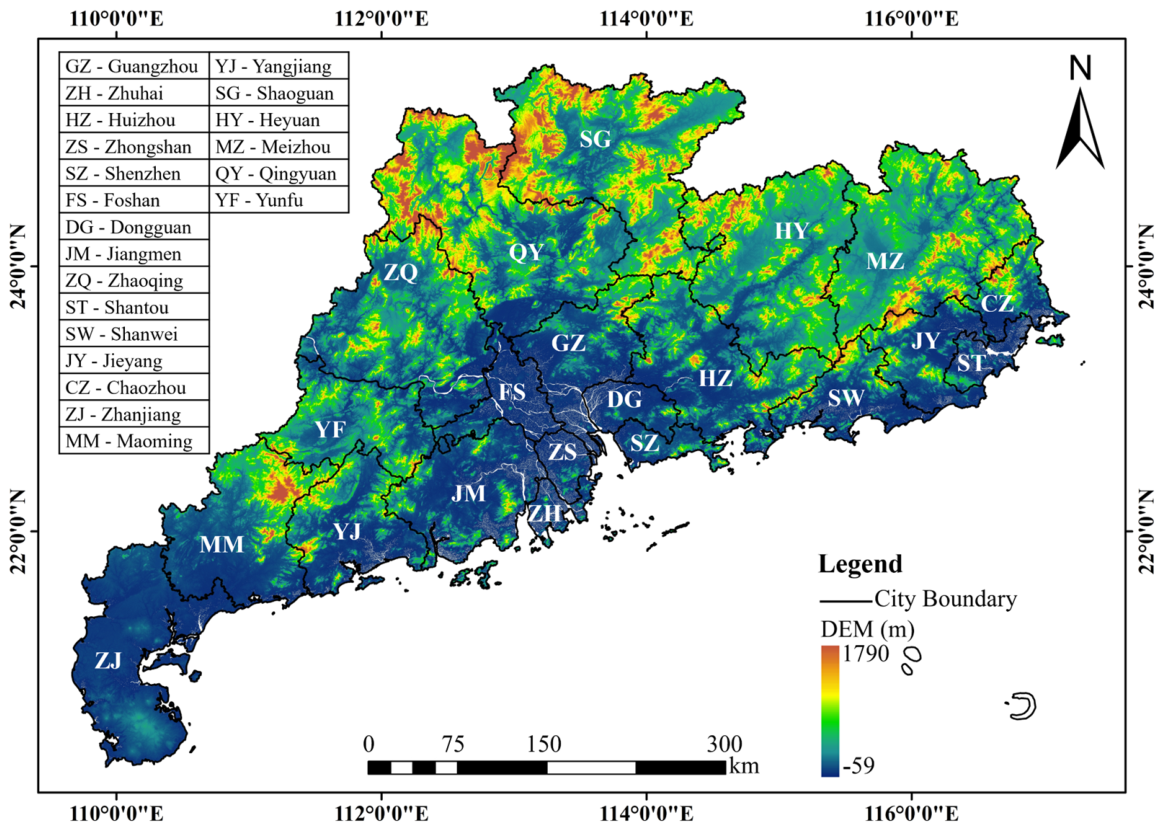
Cropland resources in Guangdong have long been under significant constraints. Over the past three decades of rapid urbanization, extensive conversion of cropland to built-up areas has occurred, accompanied by quantitative loss, spatial displacement, and landscape fragmentation [34,35,36]. The province’s prominent human–land conflicts, limited reserve cropland resources, and frequent agricultural restructuring have further intensified the pressure on cropland systems [36]. Moreover, marked disparities in natural conditions and socioeconomic development exist across the region. The Pearl River Delta core urban agglomeration contrasts sharply with the less developed eastern, western, and northern Guangdong, where cropland use patterns and functions differ considerably [37]. Consequently, continuous and detailed monitoring of cropland use changes has become critically important. The topographic and administrative divisions of the study area are presented in Figure 1, with city abbreviations defined in the embedded table. The topographic data was obtained from the NASA SRTM 30 m Digital Elevation Model (DEM).

In accordance with the Guangdong Provincial Territorial Spatial Planning (2021–2035), the province is delineated into four major agricultural functional zones: the Pearl River Delta Metropolitan Agricultural Zone (PRD-MAZ), the Eastern Guangdong Precision Agricultural Zone (EGD-PAZ), the Western Guangdong High-Efficiency Agricultural Zone (WGD-HEAZ), and the Northern Guangdong Ecological and Specialty Agricultural Zone (NGD-ESAZ). This four-zone framework reflects the region’s pronounced spatial heterogeneity in both physical geography and agricultural functions, with distinct cropland use characteristics observed across different zones [37,38]. Based on this planning framework and complemented by relevant municipal-level territorial spatial plans and agricultural zoning outcomes, the 21 prefecture-level cities of the province are integrated into the four agricultural zones. Notably, Zhaoqing City is divided due to its pronounced physiographic and functional heterogeneity. Its southeastern districts and county-level cities (Duanzhou, Dinghu, Gaoyao, and Sihui) are assigned to the PRD-MAZ, while the counties of Fengkai, Huaiji, Guangning, and Deqing fall under the NGD-ESAZ. This subdivision is consistent with the Zhaoqing Municipal Territorial Spatial Planning (2021–2035) and Zhaoqing’s 14th Five-Year Plan for Agricultural and Rural Modernization. A detailed summary of the four agricultural zones is provided in

Table 1. Overview of the four agricultural function zones in Guangdong Province.

Agricultural Function Zone	Included Cities (Counties/Districts)		Agricultural Positioning and Main Characteristics of Cropland Use
Pearl River Delta Metropolitan Agricultural Zone (PRD-MAZ)	Guangzhou (GZ)	Shenzhen (SZ)	Positioned as peri-urban high-value agriculture, integrating efficient production, ecological conservation, and leisure tourism. This zone faces extreme urbanization pressure, leading to significant cropland loss and spatial displacement, resulting in highly fragmented patches.
	Zhuhai (ZH)	Foshan (FS)
	Huizhou (HZ)	Dongguan (DG)
	Zhongshan (ZS)	Jiangmen (JM)
	Zhaoqing (ZQ)	Gaoyao (GY)
	Duanzhou (DZ)	Sihui (SH)
	Dinghu (DH)
Eastern Guangdong Precision Agricultural Zone (EGD-PAZ)	Shantou (ST)		Rooted in traditional intensive farming, focusing on specialty fruits, vegetables, tea, and aquaculture. Per capita cropland is extremely limited, and fields are characteristically small and fragmented, though traditional farming patterns are stable.
	Shanwei (SW)
	Chaozhou (CZ)
	Jieyang (JY)
Western Guangdong High-Efficiency Agricultural Zone (WGD-HEAZ)	Zhanjiang (ZJ)		Leverages abundant solar–-thermal resources and land advantages to emphasize large-scale, high-efficiency production of tropical fruits and winter vegetables. Cropland is relatively contiguous and generally stable in quantity.
	Maoming (MM)
	Yangjiang (YJ)
Northern Guangdong Ecological & Specialty Agricultural Zone (NGD-ESAZ)	Shaoguan (SG)	Heyuan (HY)	Functions as a mountainous characteristic agriculture zone and ecological protection zone, producing forest fruits, tea, and quality rice. Cropland is scattered across intermontane basins and valleys, with use patterns significantly constrained by both topography and ecological conservation requirements.
	Meizhou (MZ)	Qingyuan (QY)
	Yunfu (YF)
	Zhaoqing (ZQ)	Fengkai (FK)
	Guangning (GN)	Huaiji (HJ)
	Deqing (DQ)

.

2.2. Data and Processing

2.2.1. Data Sources

This study utilizes the annual 30 m land cover time series (1990–2024) from the China Land Cover Dataset (CLCD) [39], which offers consistent, temporally seamless land use data across China [40,41] and is available at the Zenodo repository [42]. The original version of CLCD has an overall accuracy of approximately 80% [39]. Updated annually to maintain temporal continuity, the dataset has been widely applied in cropland monitoring, land-use change detection, and related sustainability assessments across multiple scales in China [43,44,45,46,47]. It classifies nine categories—cropland, forest, shrub, grassland, water, snow/ice, barren, impervious, and wetland—and supports fine-scale, continuous monitoring of long-term environmental changes. In addition to the land cover data, the vector boundaries of Guangdong’s four agricultural functional zones were derived from the Guangdong Provincial Territorial Spatial Planning (2021–2035). All vector data used the GCS_WGS_1984 coordinate system. Additionally, data-related limitations and potential influences are discussed in Section 4.2.

The 35-year study period (1990–2024) comprises seven consecutive five-year intervals: 1990–1994, 1995–1999, 2000–2004, 2005–2009, 2010–2014, 2015–2019, and 2020–2024. The choice of a five-year interval is motivated by multiple considerations. First, it aligns with China’s national and provincial land use and agricultural planning cycles (e.g., the “Five-Year Plan” framework), facilitating the translation of analytical results into actionable policy recommendations. Second, the five-year threshold has been widely adopted in cropland dynamics research as a meaningful temporal unit for characterizing land-use persistence and change. The Food and Agriculture Organization (FAO) classifies land remaining fallow for up to five years as temporarily fallow and suggests that a maximum idle period of five years is generally suitable for distinguishing temporarily fallow land from land requiring reclassification [48]. This five-year threshold has also been adopted as an operational criterion for cropland abandonment in numerous remote sensing-based studies [49,50,51,52,53,54]. Third, while previous national-scale cropland studies have commonly adopted decadal intervals to capture broad macro-level trends across China’s vast territory [5,7,55,56], a finer temporal resolution is desirable at the regional scale, where cropland dynamics are more sensitive to localized urbanization pressures, agricultural restructuring, and policy interventions. The five-year interval offers a compromise between temporal granularity and data stability, enabling the detection of relatively timely changes while remaining grounded in common methodological practices [57,58,59,60,61].

Within each five-year interval, the complete series of annual land cover maps were used for computing stability indicators. A pixel-tracking strategy was applied to capture the temporal trajectory of each cropland pixel, while landscape-level metrics were aggregated from annual computations to characterize the average spatial configuration over the five-year period. To assess whether the main findings are sensitive to the choice of the five-year window, we conducted an additional robustness check using a three-year interval (covering 1990–2022) with all computational procedures held constant. The results were broadly consistent across the two temporal aggregation schemes. Specifically, Spearman correlations between the five-year and three-year schemes were 0.968 for city-level mean stability, 0.8849 for city-level quadrant classifications, and 0.8262 for transition probabilities. The low point in the provincial stability trajectory recurred in the 2005–2007 interval under the three-year window. The quadrant-wise comparison showed the same broad grouping of cities, though with a reversal in the ordering of the two divergent quadrants (see Section 4.2 and Supplementary Materials Text S1 for details). This analysis suggests that the primary conclusions of this study are not substantially altered by the specific choice of the five-year window.

2.2.2. Data Processing

Land cover data were harmonized to a common spatial framework. The CLCD annual maps use an Albers projection, whereas the vector boundaries of Guangdong Province, the four agricultural functional zones, and the 21 prefecture-level cities were originally in the GCS_WGS_1984 geographic coordinate system. All vector boundaries were projected to match the CLCD Albers projection, and binary raster masks were created for each of the 26 analysis units. The masks were stored as independent files to streamline repeated extraction during subsequent pixel-level computations. Annual CLCD images were also clipped to the effective extent of Guangdong Province after verifying their spatial consistency across all 35 years.

For each five-year period, we derived two complementary streams of information from the annual land cover data to support the subsequent stability assessment (see Section 2.3 for details). First, we calculated the total cropland area within each analysis unit for each year by intersecting the cropland layer with the corresponding mask. This yielded a time series of annual cropland area for each unit, forming the basis for the quantity stability indicators. Second, we retained the spatial distribution of cropland pixels within each unit for each year, allowing for subsequent analysis of cropland configuration and pixel-level dynamics. All extractions were performed using the original 30 m resolution raster data to preserve spatial detail.

All raster processing and indicator extraction was implemented in MATLAB R2023a, using pre-cached mask and vectorized operations to improve computational efficiency. The binary masks created for each analysis unit were used in two ways throughout the subsequent indicator extraction. First, for annual cropland extraction, each year’s land cover image was masked to the extent of each analysis unit, so that only pixels within the unit were retained for cropland identification. This ensures that all area calculations and pixel-based statistics are confined to the spatial boundaries of each unit. Second, for indicators requiring neighbor-based calculations, the mask defines the effective analysis domain. Pixels outside the mask are treated as non-cropland, and the mask ensures that no calculations are performed on cells outside the study extent. This masking approach is consistently applied across all analysis units and all years, maintaining the spatial consistency and comparability of the computed metrics. The resulting multi-scale indicator values (at province, agricultural zones, and cities levels) were exported in structured CSV files. Statistical graphics and maps were produced using Origin 2024, Python 3.12 and ArcMap 10.8.

2.3. Methods

2.3.1. Cropland Use Stability Assessment Framework

In this study, cropland use stability is defined as the capacity of cropland resources to maintain a consistent state of use in terms of both quantity and spatial location over a given time span. To systematically capture this capacity, we constructed a quantity–spatial two-dimensional assessment framework. The period from 1990 to 2024 was divided into seven consecutive five-year intervals. Within each interval, we utilized the annual land cover data by extracting both the annual cropland area and the annual spatial distribution of cropland pixels for each analysis unit.

For the quantity stability dimension ($S_1$), we selected four indicators—coefficient of variation ($CV$), accumulated change intensity ($ACI$), trend slope ($\beta$), and rate of change ($ROC$)—to characterize area fluctuation, cumulative change, and temporal trend over the five-year period. For the spatial stability dimension ($S_2$), we selected four indicators—weighted persistence frequency ($WPF$), cropland neighborhood density ($CND$), trajectory variability ($TV$), and edge density ($ED$)—to characterize cropland persistence, spatial aggregation, trajectory consistency, and patch configuration. Detailed definitions and formulas for all indicators are provided in Section 2.3.2.

The eight selected indicators address two fundamental aspects of cropland use stability: the maintenance of cropland area over time (quantity stability) and the persistence of cropland at specific locations (spatial stability). These two aspects have been widely recognized as core components in recent cropland stability evaluation frameworks [13,25,26,29]. Operationally, the four quantity indicators reflect different aspects of temporal dynamics: $CV$ measures interannual fluctuation around the mean, $ACI$ quantifies cumulative deviation from the initial state, $\beta$ characterizes the direction and magnitude of the overall trend, and $\mathit{ROC}$ reflects the average rate of year-to-year change. For the spatial dimension, the four indicators similarly capture distinct facets: $\mathit{WPF}$ directly measures locational persistence, $\mathit{CND}$ captures local aggregation, $\mathit{TV}$ quantifies pixel-level trajectory consistency, and $\mathit{ED}$ reflects boundary complexity and fragmentation intensity. While landscape metrics such as patch density or mean patch size are also commonly used, $\mathit{ED}$ is preferred here because it is less sensitive to classification noise in medium-resolution (30 m) time-series data. Moreover, it effectively captures the edge related disturbance that directly affects spatial stability in fragmented peri-urban landscapes. The selected indicator set thus systematically characterizes both the temporal dynamics and the spatial organization of cropland use without introducing redundant or data-sensitive metrics.

For each dimension, the selected indicators were normalized and then synthesized to obtain dimension-specific stability indices ($S_1$ and $S_2$). An integrated cropland use stability index ($S$) was subsequently derived by aggregation of $S_1$ and $S_2$, and classified into stability levels to support multiscale spatiotemporal analysis. The detailed calculation procedures—including standardization, entropy weighting, sensitivity analyses, and classification—are presented in Section 2.3.2 and Section 2.3.3. All indicator calculations were performed using the pre-generated masks for each analysis unit, ensuring that all computations are confined to the respective spatial extents and that pixels outside the mask are consistently treated as non-cropland.

2.3.2. Indicator System and Computation of Dimension-Specific Stability Indices

Based on the above framework, eight indicators were selected to construct the evaluation system, four for the quantity dimension and four for the spatial dimension. The complete set of indicators, along with their formulas and interpretations, is presented in

Table 2. Indicators for cropland use stability assessment.

Dimension	Indicator (Abbreviation)	Formula		Interpretation
$S_1$	Coefficient of Variation ($CV$)	$CV={\displaystyle \frac{\sigma }{\mu }}\times 100\%$	(1)	Reflects the relative interannual fluctuation of cropland area. A smaller value indicates more stable area over time.
	Accumulated Change Intensity ($\mathit{ACI}$)	$ACI={\displaystyle \frac{\sum \left|A_{t+1}-A_t\right|}{A_1}}\times 100\%$	(2)	Measures the total cumulative change relative to the initial area. A smaller value indicates lower cumulative change and higher stability.
	Trend Slope ($\beta$)	$A_t=\beta \times t+\alpha +\epsilon$	(3)	Captures the monotonic trend direction and magnitude. A smaller absolute value indicates a weaker temporal trend.
	Rate of Change ($\mathit{ROC}$)	$ROC={\displaystyle \frac{1}{n-1}}\times {\sum }_{t=1}^{n-1}\left|{\displaystyle \frac{A_{t+1}-A_t}{A_t}}\right|\times 100\%$	(4)	Represents the average interannual relative change rate. A smaller value indicates less volatility and higher stability.
$S_2$	Weighted Persistence Frequency ($\mathit{WPF}$)	$WPF={\displaystyle \frac{{\sum }_{k=1}^5(f_k\times w_k)}{N}}$ $w_k={\displaystyle \frac{k}{5}}$	(5)	Higher values indicate stronger persistence of cropland at specific locations, laying a solid foundation for spatial pattern stability.
	Cropland Neighborhood Density ($\mathit{CND}$)	$CND={\displaystyle \frac{1}{N}}\times {\sum }_{i=1}^N{\displaystyle \frac{{\sum }_{j\in {\mathsf{\Omega }}_i}{x}_j}{8}}$	(6)	Measures the local spatial aggregation of cropland. A higher value indicates stronger clustering and more stable spatial configuration.
	Trajectory Variability ($\mathit{TV}$)	$TV={\displaystyle \frac{1}{N}}\times {\sum }_{i=1}^{N}Var\left(T_i\right)$	(7)	Measures the temporal variance of each pixel’s cropland status over the five-year sequence. A smaller value indicates more stable land-use decisions at the pixel level.
	Edge Density ($\mathit{ED}$)	$\mathit{ED}={\displaystyle \frac{E}{A}}\times 10000$	(8)	Describes the complexity of cropland patch boundaries. A smaller value indicates more compact and less fragmented patches.

.

In Table 2, $A_t$ denotes the cropland area (km²) in year $t$; $\sigma$ and $\mu$ are the standard deviation and mean of $A_t$ over the five-year period. For $ACI$, $A_1$ is the area in the first year of the period. For $\beta$, $t$ is the time sequence from 1 to 5, representing the five consecutive years within the period. For $ROC$, $n=5$, the summation is taken over the four adjacent year pairs within the period. For $WPF$, $f_k$ is the number of cropland pixels (identified in the first year) that persisted for exactly $k$ years ($k$ = 1, …, 5), and $N$ is the total number of cropland pixels in the first year. For $CND$, $x_j\in \left\{\mathrm{0,1}\right\}$ indicates whether pixel $j$ is cropland, and ${\Omega }_i$ denotes the 8-neighborhood surrounding pixel $i$; the term $\left({\sum }_{j\in {\Omega }_i}{x}_j)/8\right.$ gives the proportion of cropland pixels in that neighborhood, and $N$ refers to the number of cropland pixels in that year, which varies annually. For $TV$, $N$ is the total number of initial cropland pixels, $T_i=\left[T_1,T_2,\dots ,T_5\right]$ is the five-year state sequence of pixel $i$, with each $T_i\in \left\{\mathrm{0,1}\right\}$ (1 = cropland, 0 = non-cropland), and $Var\left(T_i\right)$ is the variance of this sequence. For $ED$, $E$ is the total edge length (m) calculated using a 4-neighbor rule (i.e., counting edges between cropland and non-cropland pixels in the four cardinal directions), with each pixel edge measuring 30 m; $A$ is the total cropland area (ha); the factor of 10,000 converts the unit from m/ha to the conventional scale of edge density; and the reported value is the average over the five years within each period.

The indicator values in Table 2 were computed using the pre-generated masks described in Section 2.2.2. For neighbor-based calculations, cells outside the mask were treated as non-cropland. More specifically, $CND$ was calculated annually for each year within the five-year interval and then averaged over the five years. For each year, cells outside the analysis unit mask were treated as non-cropland in the 8-neighborhood calculation, and the denominator was fixed at 8 for all pixels, including boundary pixels. $CND$ is recalculated annually from the current year’s cropland extent. Therefore, newly appeared cropland pixels are included in the $CND$ values for the year(s) in which they appear. For $WPF$, the calculation tracks only pixels classified as cropland in the first year of each five-year interval. This aligns with its purpose of assessing the persistence of existing cropland at specific locations. Newly appearing cropland is not included in the $WPF$ denominator. This design choice is complementary to $CND$: the former captures locational persistence, while the latter captures the spatial context of all cropland present in each year.

To construct the dimension-specific stability indices, all selected indicators were first computed from the annual land cover data for each analysis unit and each five-year period, yielding raw indicator values for $S_1$ ($CV$, $\mathit{ACI}$, $\beta$, $\mathit{ROC}$) and $S_2$ ($\mathit{WPF}$, $\mathit{CND}$, $\mathit{TV}$, $\mathit{ED}$). For the quantity dimension, the trend slope $\beta$ was converted to absolute value $\left|\beta \right|$ to represent the magnitude of the temporal trend regardless of direction, as both positive and negative trends indicate change away from stability.

All raw indicator values were standardized and normalized to ensure comparability, with the detailed formulas provided in the Supplementary Materials (Text S2). Directional adjustments were then applied so that larger values consistently indicate higher stability. For the quantity dimension, all four indicators—$CV$, $\mathit{ACI}$, $\left|\beta \right|$, $\mathit{ROC}$—are inherently instability-oriented and were transformed as $x^{\prime }=1-x$. For the spatial dimension, $\mathit{WPF}$ and $\mathit{CND}$ are inherently positive indicators (larger = more stable), whereas $\mathit{TV}$ and $\mathit{ED}$ are negative indicators (smaller = more stable). The latter two were accordingly transformed as $x^{\prime }=1-x$, while $\mathit{WPF}$ and $\mathit{CND}$ were left unchanged. All transformed values were clipped to [0,1] to correct for minor numerical rounding errors.

Indicator weights were determined using the entropy weight method, which assigns higher weights to indicators with greater variability across observations (26 units $\times$ 7 periods). The detailed derivation of the entropy weights is provided in Supplementary Materials (Text S2). To examine the robustness of the aggregation results, we compared multiple weighting schemes for both dimensions; the full sensitivity comparison, including Spearman correlation matrices for all configurations, is provided in the Supplementary Materials (Text S3). The entropy-based dimension scores were highly consistent with all alternative schemes for both $S_1$ and $S_2$. Minimum Spearman correlations across all pairwise comparisons were 0.9768 for $S_1$ and 0.9498 for $S_2$. This confirms that the dimension-specific stability indices are robust to the choice of sub-indicator weights. The entropy-based weighting scheme was therefore selected for both dimensions. The entropy weights for $S_1$ were [$CV$: 0.334, $\mathit{ACI}$: 0.236, $\left|\beta \right|$: 0.122, $\mathit{ROC}$: 0.308], and for $S_2$ were [$\mathit{WPF}$: 0.149, $\mathit{CND}$: 0.296, $\mathit{TV}$: 0.160, $\mathit{ED}$: 0.395].

2.3.3. Integration of Dimension-Specific Indices and Stability Classification

With the dimension-specific stability indices ($S_1$ and $S_2$) obtained from Section 2.3.2, this subsection integrates them into a composite index ($S$) and classifies the stability grades. To ensure numerical comparability between the two dimensions, $S_1$ and $S_2$ were first normalized to the [0,1] interval using min–max normalization. The integrated stability index ($S$) was then calculated as the weighted sum of the normalized dimension indices:

$$S=w_1\times {S_1}^{\prime }+w_2\times {S_2}^{\prime }$$

(9)

where ${S_1}^{\prime }$ and ${S_2}^{\prime }$ are the min–max-normalized quantity stability index and spatial stability index, respectively, and $w_1$ and $w_2$ are their respective weights, satisfying $w_1+w_2=1$.

To determine the appropriate weighting scheme, we compared six configurations (

Table 3. Sensitivity analysis of $S_1$–$S_2$ weighting schemes.

Scheme	w1	w2	Spearman’s ρ vs. Entropy Scheme
Entropy	0.386	0.614	1.000
Equal	0.5	0.5	0.987
$S_1$_0.6	0.6	0.4	0.953
$S_2$_0.6	0.4	0.6	1.000
$S_1$_0.7	0.7	0.3	0.898
$S_2$_0.7	0.3	0.7	0.991

): entropy-based (derived from the relative variability of $S_1$ and $S_2$), equal weighting (0.5/0.5), and four asymmetric schemes (0.7/0.3, 0.3/0.7, 0.6/0.4, and 0.4/0.6) for sensitivity testing. As shown in Table 3, the Spearman correlation coefficients between the entropy-based scheme and all alternative schemes were consistently high, indicating that the overall rankings of cropland use stability are robust to the choice of weighting between the two dimensions. The entropy-based scheme was therefore adopted. The entropy-based weights, based on all 182 observations (26 units $\times$ 7 periods), yielded $w_1=0.386$ and $w_2=0.614$, reflecting the greater informational variability in the spatial dimension across the study units.

The integrated stability index $S$ ranges from 0 to 1, with higher values indicating greater cropland use stability. To facilitate interpretation and policy application, the 21 prefecture-level cities were classified into five grades. We compared three classification methods and adopted the Jenks method because it maximizes between-class differences while minimizing within-class variance (see Supplementary Materials Text S3 for detailed comparisons). The $S$ values from all 21 cities across the seven study periods (147 observations in total) were pooled to derive global breakpoints. These breakpoints were then applied to classify each city–period combination into five grades: Low (L), Relatively Low (RL), Moderate (M), Relatively High (RH), and High (H), ensuring consistent temporal comparability across all periods. The resulting breakpoints were [0.5703, 0.6544, 0.7057, 0.7641] for the five classes.

From a management perspective, a “High” stability grade indicates that cropland in the city maintained both stable area and persistent spatial configuration over the five-year interval, suggesting suitability for priority designation as permanent basic farmland with minimal intervention. A “Relatively High” or “Moderate” grade implies partial stability, calling for targeted monitoring of the weaker dimension—quantity or space—depending on the city’s specific situation. A “Relatively Low” or “Low” grade signals substantial instability, necessitating diagnostic assessment to identify whether the primary pressure is area loss, fragmentation, or both, and informing differentiated interventions such as stricter occupation control, land consolidation, or ecological restoration.

3. Results

3.1. Temporal Evolution of Integrated Cropland Use Stability at the Provincial Scale

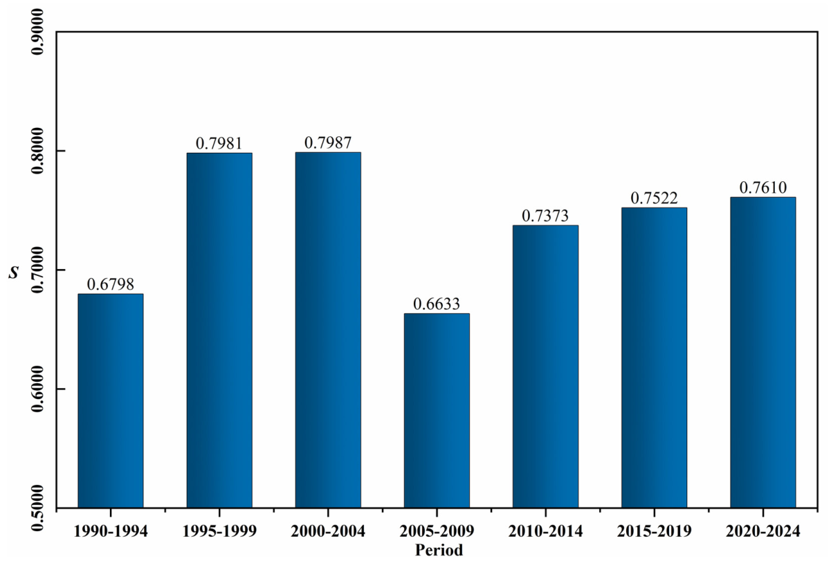
Based on the constructed two-dimensional assessment framework, the integrated cropland use stability index ($S$) for Guangdong Province was calculated across seven study periods from 1990 to 2024, with the temporal trend illustrated in Figure 2.

The provincial integrated stability index exhibited notable temporal fluctuations over the 35-year study period, with $S$ values ranging from 0.6633 to 0.7987 and a mean of 0.7415 across the seven periods. In terms of overall trajectory, the $S$ value followed a “rise–sharp decline–gradual recovery” pattern. During the first three periods (1990–1994, 1995–1999, and 2000–2004), the $S$ values increased from 0.6798 to 0.7987. The latter two of these periods remained nearly stable at the highest level of the entire time series. This suggests that provincial cropland use stability was generally high and steadily improving throughout the 1990s and into the early 2000s. However, during the fourth period (2005–2009), the $S$ value dropped sharply to 0.6633, a decline of 16.9% from the preceding period and the lowest point of the entire study. This indicates significant disturbance to the cropland use system and a marked weakening of integrated stability. From the fifth period onward (2010–2014, 2015–2019, and 2020–2024), the $S$ value rebounded and exhibited a slowly ascending trend, increasing from 0.7373 to 0.7610, suggesting a gradual recovery of provincial cropland stability in the most recent 15 years. Notably, the values of the last two periods both exceeded the study-period mean of 0.7415, indicating that the provincial integrated stability has stabilized at a relatively high level in recent years.

Overall, the integrated cropland use stability in Guangdong Province exhibited a fluctuating yet generally positive trajectory over the 35 years. It increased from 0.6798 in the initial period to 0.7610 in the final period, representing a cumulative increase of about 12.0%. The change process was not a monotonic improvement but rather a trajectory characterized by steady increase, a sharp decline during 2005–2009, and a subsequent gradual recovery. The pronounced degradation during the 2005–2009 period represents a critical time window meriting particular attention, while the sustained recovery observed in the last three periods suggests a positive trend in cropland stability. This macro-level trend provides a provincial-scale reference for subsequent in-depth exploration of stability differentiation patterns at the agricultural zone and prefecture-level city scales.

3.2. Differentiation of Integrated Cropland Use Stability Across the Agricultural Zones

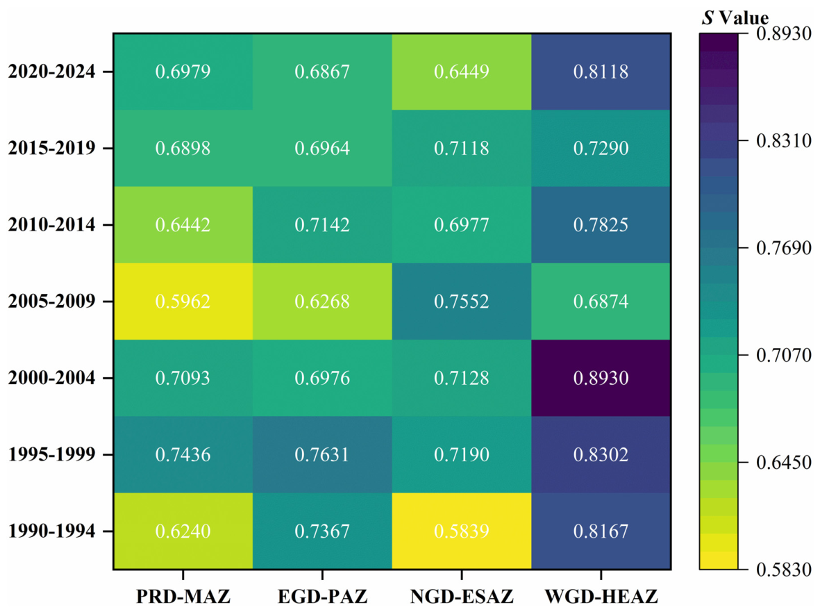
At the scale of the four major agricultural functional zones in Guangdong Province, the integrated cropland use stability index ($S$) exhibited pronounced regional differentiation and distinct temporal evolution trajectories (Figure 3). Overall, the WGD-HEAZ consistently maintained the highest integrated stability throughout the study period, whereas the other three zones exhibited varying degrees of fluctuations with notable declines during the mid-study period.

In terms of stability levels, the four zones can be broadly divided into two tiers. The WGD-HEAZ maintained persistently high stability across all seven periods, with $S$ values ranging from 0.6874 to 0.8930 and a multi-period mean of 0.7929. This far exceeded those of the other three zones and demonstrated superior stability retention. Within this zone, the $S$ value reached its peak during the third period (2000–2004) at 0.8930 and its lowest during the fourth period (2005–2009) at 0.6874. While this trough remained higher than the mean values of the NGD-ESAZ (0.6893) and the PRD-MAZ (0.6721), it was slightly lower than the EGD-PAZ mean of 0.7031. The remaining three zones—EGD-PAZ, NGD-ESAZ, and PRD-MAZ—formed a second tier, with mean $S$ values of 0.7031, 0.6893, and 0.6721, respectively. These zones fluctuated within a relatively close range over the 35 years, though their temporal trajectories exhibited marked differences in phase and amplitude.

With respect to evolution patterns, three typical types can be identified. The first is the sustained high-stability type, represented by the WGD-HEAZ. Its integrated stability remained at a high level throughout the study period; although a moderate decline occurred during the 2005–2009 period, it rebounded strongly thereafter and reached 0.8118 in the final period (2020–2024), indicating strong system resilience. The second is the fluctuating recovery type, represented by the EGD-PAZ and the PRD-MAZ. Both zones experienced a sharp decline during the 2005–2009 period—the PRD-MAZ dropped from 0.7093 to 0.5962 (a 15.9% decline), while the EGD-PAZ fell from 0.6976 to 0.6268 (a 10.1% decline). However, their post-decline trajectories diverged noticeably. The PRD-MAZ exhibited a steady and sustained recovery over the subsequent three periods, reaching 0.6979 by 2020–2024. By contrast, the EGD-PAZ rebounded rapidly during the 2010–2014 period (to 0.7142) but showed a slight downward trend in the last two periods, stabilizing at approximately 0.6867. The third type is the relatively stable type, represented by the NGD-ESAZ, where $S$ values ranged from 0.5839 to 0.7552 across all periods. This range was wider than that of the PRD-MAZ, but the zone exhibited no abrupt decline events. This suggests an adaptive improvement in cropland use stability following the early 1990s, with the absence of sharp degradation being the defining feature of its relative stability. Notably, the NGD-ESAZ exhibited the lowest stability in the initial period (1990–1994) at 0.5839 but quickly rose and maintained moderate levels thereafter.

Collectively, the stability differentiation pattern across the four agricultural zones reveals a complex relationship between regional characteristics and cropland use stability. The WGD-HEAZ, characterized by relatively contiguous cropland and large-scale agricultural production, maintained the most enduring stability. The NGD-ESAZ, dominated by mountainous ecological agriculture, demonstrated relatively moderate fluctuations with no abrupt degradation events. In contrast, the PRD-MAZ and the EGD-PAZ, both subject to intensive urbanization pressure and agricultural restructuring, experienced pronounced declines during the 2005–2009 period. The PRD-MAZ showed a slower recovery trajectory, whereas the EGD-PAZ exhibited a more volatile post-decline pattern. This spatial and temporal heterogeneity underscores the need for differentiated cropland management strategies tailored to the specific stability dynamics of each agricultural zone.

3.3. Spatial Patterns and Evolution of Integrated Cropland Use Stability at the Prefecture-Level City Scale

3.3.1. Spatial Differentiation of Integrated Stability and Evolution Types

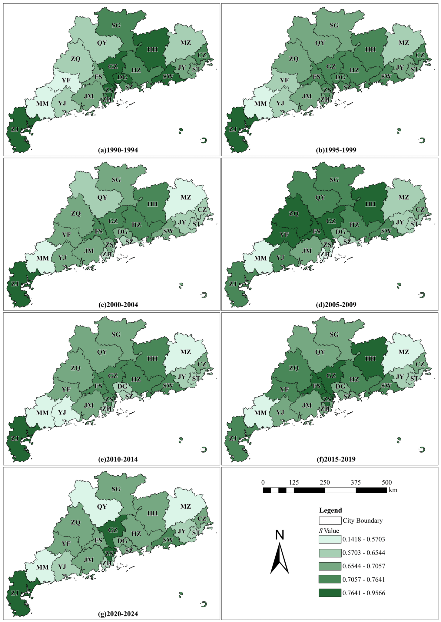
At the scale of the 21 prefecture-level cities, integrated cropland use stability exhibited marked spatial heterogeneity and dynamic reorganization over the 35-year study period (Figure 4). The stability grade distribution maps across the seven study periods reveal spatial heterogeneity, with the relative positions of high- and low-stability cities shifting over time and moderate-stability cities forming the transitional matrix of the overall spatial pattern.

Table 4. Integrated cropland use stability index ($S$) of the 21 prefecture-level cities across the seven study periods.

City	1990–1994	1995–1999	2000–2004	2005–2009	2010–2014	2015–2019	2020–2024	Average
GZ	0.8116	0.7433	0.8168	0.8210	0.8000	0.7636	0.7778	0.7906
SG	0.6722	0.6387	0.7547	0.7067	0.6569	0.6903	0.6675	0.6839
SZ	0.6893	0.7939	0.6665	0.5702	0.6256	0.6948	0.7042	0.6816
ZH	0.7006	0.5564	0.6251	0.4297	0.6184	0.6528	0.6490	0.6046
ST	0.5653	0.6132	0.5543	0.5162	0.5923	0.5830	0.5706	0.5707
FS	0.6109	0.8016	0.8249	0.7846	0.7723	0.7615	0.6885	0.7492
JM	0.6097	0.6904	0.7481	0.6114	0.6435	0.6828	0.6774	0.6662
ZJ	0.9024	0.9403	0.9566	0.7247	0.8815	0.7387	0.8527	0.8567
MM	0.1418	0.2611	0.4643	0.4661	0.4997	0.4320	0.5090	0.3963
ZQ	0.4229	0.6826	0.7326	0.7758	0.6998	0.7354	0.6903	0.6771
HZ	0.7420	0.7440	0.7910	0.7282	0.7271	0.7287	0.6854	0.7352
MZ	0.3738	0.4399	0.4551	0.5295	0.5003	0.5228	0.4923	0.4734
SW	0.8131	0.7862	0.7332	0.7040	0.7435	0.7261	0.7245	0.7472
HY	0.7777	0.7399	0.8034	0.7832	0.7657	0.7642	0.7019	0.7623
YJ	0.4432	0.5115	0.7440	0.6978	0.4634	0.6632	0.6277	0.5930
QY	0.4913	0.6500	0.6198	0.7225	0.6510	0.6906	0.4833	0.6155
DG	0.7805	0.7788	0.6944	0.6217	0.6276	0.6965	0.6731	0.6961
ZS	0.7903	0.7412	0.7620	0.6178	0.7346	0.7621	0.7734	0.7402
CZ	0.7336	0.7483	0.6696	0.6341	0.6370	0.6777	0.6882	0.6841
JY	0.5688	0.6267	0.5933	0.5395	0.6208	0.6244	0.5934	0.5953
YF	0.2080	0.4063	0.7690	0.7884	0.6357	0.7428	0.7003	0.6072

presents the integrated cropland use stability index for the 21 prefecture-level cities across the seven study periods. For each city–period, the computed index values are rounded to four decimal places; the city-specific mean is then derived from these rounded values and likewise rounded to four decimals.

From the perspective of the overall spatial pattern, Zhanjiang City (ZJ) in western Guangdong consistently ranked as the area with the highest integrated cropland use stability across the entire province, with a multi-period mean $S$ value of 0.8567, far exceeding that of other cities. However, it was not consistently the highest in every period: Guangzhou (GZ) surpassed Zhanjiang in the 2005–2009 period and again in 2015–2019, making these two cities the alternating leaders in provincial cropland stability. Other high-stability cities include Heyuan (HY, mean 0.7623), Foshan (FS, mean 0.7492), Shanwei (SW, mean 0.7472), Zhongshan (ZS, mean 0.7402), and Huizhou (HZ, mean 0.7352), all of which maintained relatively high stability levels across most periods. In contrast, the lowest stability values were predominantly observed in Maoming (MM, mean 0.3963), Meizhou (MZ, mean 0.4734), Shantou (ST, mean 0.5707), Yangjiang (YJ, mean 0.5930), and Jieyang (JY, mean 0.5953). Among these, Maoming exhibited exceptionally low values in the early periods (0.1418 in 1990–1994 and 0.2611 in 1995–1999), followed by a gradual increase that remained consistently below 0.5100 across all seven periods, indicating persistent weakness in cropland use stability. Meizhou similarly remained within a low range of 0.3738 to 0.5295 throughout the study period, with no significant recovery.

Examining the spatial process of grade transitions over time, several patterns emerge. In the early periods (1990–1999), cities with relatively high stability were widely distributed across western Guangdong (ZJ), the Pearl River Delta (GZ, HZ, DG, ZS), and parts of eastern Guangdong (SW, HY). By the middle period (2005–2009), a pronounced low-stability cluster emerged in the core Pearl River Delta cities—most notably Zhuhai (0.4297), Shenzhen (0.5702), and Dongguan (0.6217)—as well as in parts of eastern Guangdong (ST at 0.5162, JY at 0.5395). This low-stability cluster persisted and appeared to expand in spatial continuity during the later periods, while the high-stability cores centered on Zhanjiang and Guangzhou remained relatively stable but increasingly geographically isolated.

3.3.2. Stability Grade Transition Matrix Analysis

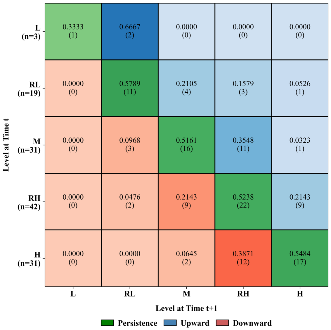
To quantify the dynamic transitions of integrated cropland use stability grades between adjacent periods, a grade transition probability matrix was constructed based on the grade changes of the 21 prefecture-level cities across the seven study periods (Figure 5). Stability grades were classified into five levels—Low (L), Relatively Low (RL), Moderate (M), Relatively High (RH), and High (H)—using the Jenks natural breaks method (detailed in Section 2.3.3). In the matrix, rows represent the grade of the preceding period and columns the grade of the subsequent period. Each cell shows the row-conditional transition probability (i.e., proportion of transitions originating from that row) and, in parentheses, the corresponding count of transitions. The diagonal represents grade persistence, the upper triangle upward transitions (improvement), and the lower triangle downward transitions (degradation). The color scheme uses green for persistence, blue for upward, and red for downward, enabling a direct visual assessment of both direction and magnitude. The y-axis labels also indicate the total number of transitions originating from each grade (n).

Among the diagonal persistence probabilities, Relatively Low Stability (RL) ranked highest at 0.5789, followed by High Stability (H) at 0.5484, Relatively High Stability (RH) at 0.5238, Moderate Stability (M) at 0.5161, and Low Stability (L) at 0.3333. Cities at the L grade exhibited the lowest persistence, with a combined upward transition probability of 0.6667, predominantly shifting to RL (0.6667) with no direct transitions to M or above. For RL-grade cities, upward transitions to M (0.2105), RH (0.1579), and H (0.0526) summed to 0.421, with no downward transitions to L observed. M-grade cities showed a persistence probability of 0.5161, with upward transitions to RH (0.3548) and H (0.0323) summing to 0.3871, and downward transitions to RL (0.0968). RH-grade cities exhibited a persistence of 0.5238, with upward transitions to H (0.2143) and downward transitions to M (0.2143) and RL (0.0476). H-grade cities showed the second highest persistence (0.5484), with the only transitions being downward to RH (0.3871) and M (0.0645), and no direct transitions to RL or L.

Across the entire matrix, a total of 126 adjacent-period transitions were identified. Of these, 53.17% were persistence events, 24.60% were upward transitions, and 22.22% were downward transitions. The upward proportion (24.60%, 95% CI: 17.91–32.80%) slightly exceeds the downward proportion (22.22%, 95% CI: 15.85–30.24%), but the overlapping confidence intervals indicate that this difference is not statistically significant. Furthermore, the overall proportions are strongly influenced by the larger row counts (RH: 42, M: 31, H: 31), while the L row accounts for only three transitions; therefore, any inference about a system-wide net tendency should be interpreted with caution. Nonetheless, the row-conditional probabilities reveal several grade-specific patterns, as detailed below.

Several grade transition patterns are worth highlighting. First, L-grade cities were almost entirely observed in the early periods (1990–1994 and 1995–1999) and predominantly located in Maoming, Yunfu, and Meizhou; by the later periods, no cities remained at the L grade. Second, transitions between adjacent grades (e.g., RL$\leftrightarrow$M, M$\leftrightarrow$RH, RH$\leftrightarrow$H) accounted for the majority of off-diagonal movements, while direct transitions skipping one or more grades (e.g., L$\to$M, RL$\to$H, or H$\to$RL) were rare or absent, indicating that grade transitions tend to occur progressively. Third, the probability of upward transitions from RL to RH or H (0.2105) was lower than the probability of downward transitions from RH to M or RL (0.2619). Fourth, the H grade, once attained, exhibited a relatively high probability of persistence (0.5484), suggesting that cities reaching the highest stability level tend to maintain their status in the subsequent period.

3.3.3. Divergence Analysis Between Quantity Stability and Spatial Stability

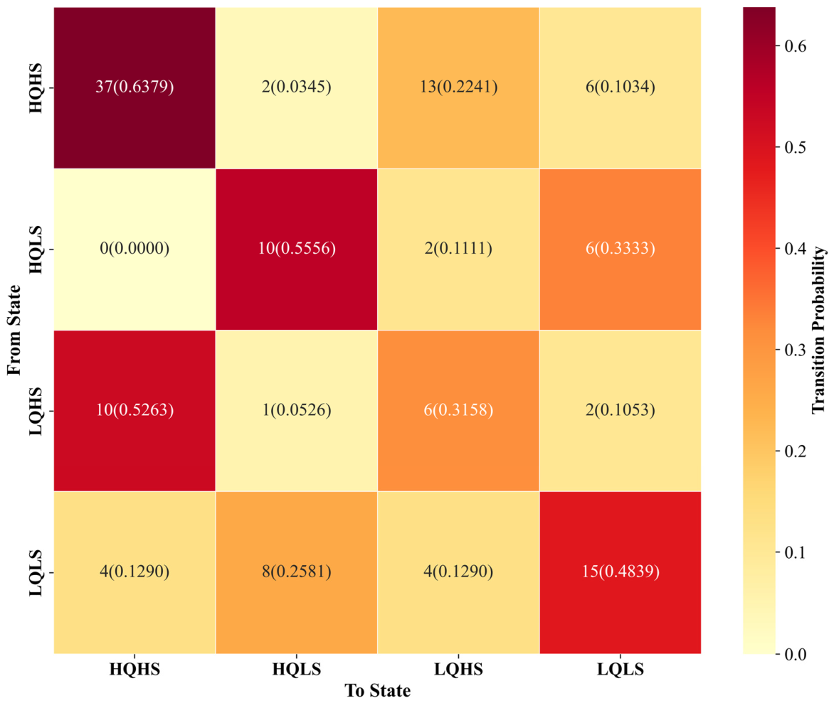
To further examine the coupling and divergence between quantity stability and spatial stability at the prefecture-level city scale, a scatter plot was constructed with the min–max-normalized quantity stability index (${S_1}^{\prime }$) on the x-axis and the spatial stability index (${S_2}^{\prime }$) on the y-axis. The individual-period scatter panels are provided in Supplementary Materials Text S4 (Figure S4a–g), while the transition probability matrix derived from these quadrant classifications is presented in Figure 6. The mean values of ${S_1}^{\prime }$ and ${S_2}^{\prime }$ across all cities in each period served as dividing lines, partitioning the coordinate space into four quadrants: High Quantity–High Spatial Synergy (HQHS), High Quantity–Low Spatial Divergence (HQLS), Low Quantity–High Spatial Divergence (LQHS), and Low Quantity–Low Spatial Synergy (LQLS). It should be noted that these quadrant thresholds are determined by the period-specific city means; hence, the resulting classifications represent relative positions within each period rather than absolute stability levels. Consequently, quadrant transitions across adjacent periods reflect changes relative to a shifting benchmark and do not necessarily indicate absolute improvement or deterioration.

Across the seven periods, the overall quadrant distribution—based on 147 city-period observations (21 cities $\times$ 7 periods)—shows that HQHS accounts for the largest share with 62 occurrences (42.18%), followed by LQLS with 35 occurrences (23.81%), LQHS with 27 occurrences (18.37%), and HQLS with 23 occurrences (15.65%). Synergistic quadrants (HQHS and LQLS combined) account for 65.99% of the total observations, while divergent quadrants (HQLS and LQHS combined) account for 34.01%, indicating that although synergistic states are more prevalent, a considerable proportion of city–periods experience dimensional divergence between quantity and spatial stability.

At the individual city level (see Supplementary Materials Text S4 for details), several contrasting trajectory patterns can be observed from the quadrant time series. Cities such as Guangzhou (GZ) and Shanwei (SW) remained in the HQHS quadrant throughout all seven periods, indicating sustained synergy between quantity and spatial stability. At the opposite end, Maoming (MM) remained in LQLS across all seven periods, reflecting persistent relative weakness in both dimensions. Heyuan (HY), Foshan (FS) and Huizhou (HZ) were predominantly in HQHS (five to six periods) but shifted to LQHS in 2020–2024, suggesting relative declines in quantity stability in recent years. Zhongshan (ZS) remained in HQHS for six of the seven periods, with the only exception being LQHS in 2005–2009. Meizhou (MZ) occupied LQLS in five of the seven periods, with two shifts to HQLS in 2005–2009 and 2015–2019. Several cities exhibited notable quadrant changes over time. Yunfu (YF) showed a marked upward trajectory, progressing from LQLS in 1990–1994 to LQHS in 1995–1999, and then to HQHS from 2000 to 2004 onward. It remained at HQHS for the periods 2005–2009, 2015–2019, and 2020–2024, with a temporary decline to LQHS during 2010–2014.

To quantify the dynamic transitions among the four quadrant types across adjacent periods, a quadrant transition probability matrix was constructed based on the 126 city–period transitions (21 cities $\times$ 6 adjacent transitions), shown in Figure 6. The diagonal persistence probabilities indicate that HQHS exhibited the highest stability among all quadrant types, with 63.79% of cities remaining in HQHS from one period to the next, markedly higher than HQLS (55.56%), LQLS (48.39%), and LQHS (31.58%). The off-diagonal transitions reveal several notable patterns. Transitions from HQHS were predominantly directed to LQHS (22.41%), with smaller proportions shifting to LQLS (10.34%) and HQLS (3.45%), suggesting that when synergy breaks down, the primary degradation pathway is a decline in quantity stability, while spatial stability remains relatively high (HQHS $\to$ LQHS). LQLS exhibited upward transitions to HQLS (25.81%), HQHS (12.90%), and LQHS (12.90%), with the highest probability directed to HQLS, indicating that quantity recovery tends to precede spatial recovery. LQHS showed a strong upward transition to HQHS (52.63%), the highest among all off-diagonal movements, while its downward transition to LQLS was only 10.53%. HQLS exhibited no upward transitions to HQHS, with its primary pathways being persistence (55.56%) and downward movement to LQLS (33.33%).

Several patterns emerging from the quadrant analysis warrant attention. First, cities in the HQLS quadrant face a potential risk of undetected spatial degradation. In this quadrant, spatial stability is low while quantity appears stable. The transition matrix shows that HQLS cities have no direct upward pathway to HQHS and a 33.33% probability of declining to LQLS in the subsequent period. Second, cities in the LQHS quadrant—where spatial stability is strong, but quantity is relatively deficient—exhibit a high probability of upward transition to HQHS (52.63%). Third, divergent conditions (HQLS and LQHS combined) are not rare phenomena but represent a persistent feature of cropland system dynamics, accounting for 34.01% of all city–period observations. The presence of such widespread divergence implies that assessments relying on a single dimension—whether quantity or spatial—may provide an incomplete picture of cropland use stability. Finally, given the moving-benchmark nature of the quadrant thresholds, observed upward or downward transitions should be interpreted as relative rank shifts among cities within each period, rather than absolute gains or losses in stability over time; caution is therefore warranted when generalizing these transition patterns to absolute policy benchmarks.

Notwithstanding these caveats, the four quadrant types may offer heuristic value for diagnostic monitoring. From a monitoring perspective, each quadrant implies a different emphasis: routine tracking for HQHS, fragmentation vigilance for HQLS, quantity recovery surveillance for LQHS, and comprehensive diagnostics for LQLS. Cities in the HQHS quadrant may benefit from continued routine monitoring, as their current synergy does not necessarily imply permanent immunity from future change. Cities in the HQLS quadrant might deserve closer attention to fragmentation-related processes—such as edge expansion or patch shrinkage—even when aggregate area statistics appear stable, as the transition matrix suggests a non-negligible risk of subsequent decline to LQLS. Cities in the LQHS quadrant may present an opportunity for monitoring whether quantity recovery occurs, given their relatively high probability of upward transition to HQHS. Cities in the LQLS quadrant may call for comprehensive diagnostic attention, as the system appears vulnerable in both quantity and space. These interpretations are derived from the observed transition patterns and should be treated as diagnostic hypotheses rather than prescriptive management mandates, particularly given the relative nature of the quadrant classification.

4. Discussion

4.1. Interpretation of the Stability Evolution Pattern

In this section we distinguish between two types of statements. Descriptive statements—such as stability values, rank orders, proportions, and transition probabilities—are directly supported by the CLCD time-series data. Interpretive statements, which link observed patterns to external drivers such as urbanization, policy shifts, agricultural restructuring, or ecological conservation, are explicitly framed as plausible inferences rather than demonstrated causal relationships, as no quantitative driver analysis was implemented in this study.

The observed spatial heterogeneity of cropland use stability in Guangdong—characterized by the persistence of high-stability areas in specific locations and the expansion of low-stability clusters in urbanizing regions—coincides temporally with the differential urbanization trajectories and agricultural functions across the province. In the Pearl River Delta core area, extensive built-up land expansion over the past three decades has been accompanied by cropland fragmentation and spatial displacement. The pronounced stability decline observed in the Pearl River Delta and eastern Guangdong agricultural zones during the 2005–2009 period aligns with a phase of accelerated urban expansion and industrial restructuring in the province; we interpret this as a plausible link to urbanization pressure. At the agricultural zone scale, the temporal difference between these two zones is notable: the Pearl River Delta experienced its most rapid urbanization and industrialization during the 1990s and early 2000s, whereas the eastern Guangdong region underwent more pronounced industrial park development and agricultural structural adjustment around 2010, coinciding with the implementation of Guangdong’s “Double Transfer” strategy. This temporal correspondence suggests that region-specific development trajectories and policy interventions may have contributed to the observed differences in disturbance timing across zones.

At the prefecture-level city scale, several distinct stability patterns merit closer examination. Zhanjiang consistently recorded the highest stability, which may be related to its abundant and relatively contiguous cropland resources in the Leizhou Peninsula, combined with less intense urbanization pressure compared with the Pearl River Delta. At the opposite end, Maoming and Meizhou both showed persistently low stability, though their trajectories differed. Maoming’s exceptionally low values in the early periods—followed by a partial recovery that remained below the provincial average—could reflect extensive conversion of cropland to orchards during the 1990s, as the city is a major producer of tropical fruits such as lychees and bananas. Meizhou’s consistently low values with little sign of recovery, on the other hand, are more likely constrained by its mountainous terrain, which results in small and highly fragmented cropland parcels. Rural labor out-migration may further reduce farming intensity and contribute to this low stability. A distinct pattern is observed in core Pearl River Delta cities such as Zhuhai, Shenzhen, and Dongguan, where stability dropped sharply during 2005–2009. This period coincided with a phase of accelerated urban expansion in the region, suggesting that intensive conversion of cropland to built-up areas may have been a contributing factor.

The grade transition matrix and the quadrant analysis both point to systematic patterns of state transitions that offer insights for stability monitoring. At the grade level, cities at intermediate stability levels tend to exhibit recurrent fluctuations rather than steady states. This suggests they are more susceptible to external disturbances than cities at either extreme. By contrast, once cities attain the highest stability grade, they tend to maintain that status in subsequent periods. This implies a possible threshold effect that stabilizes the cropland system. However, the limited number of cities achieving High Stability across the study period indicates that crossing the threshold from Relatively High to High remains uncommon. At the quadrant level, the two stability dimensions do not always move in tandem. Cities with high quantity but low spatial stability show no direct upward pathway to full synergy. However, those with low quantity but high spatial stability exhibit a relatively favorable trajectory toward recovery. This asymmetry implies that spatial persistence may provide a foundation for subsequent quantity recovery. Conversely, quantity maintenance alone—without spatial integrity—may be insufficient for long-term stability. The persistent presence of divergent conditions across all city–periods—accounting for approximately one-third of observations—indicates that such divergences are not transient anomalies. They are enduring features of the cropland system. This finding has implications for assessment design. Evaluations relying solely on a single dimension may capture only part of the overall stability status, and the combined consideration of quantity and spatial dimensions provides a more complete characterization.

4.2. Research Limitations and Future Directions

While the proposed framework provides a systematic approach for assessing cropland use stability across multiple scales, several methodological considerations and data-related limitations should be acknowledged.

Regarding data uncertainty, the 30 m spatial resolution of the CLCD data imposes limitations on capturing finely fragmented cropland patterns, particularly in the intensively cultivated areas of eastern Guangdong and the peri-urban agricultural landscapes of the Pearl River Delta. Some fine-scale patch dynamics may have been missed or misclassified. The reported overall accuracy of approximately 80% is a dataset-wide estimate; independent, year-specific validation for the post-2020 years is not explicitly documented in the original CLCD publications. In terms of potential error propagation, misclassification at cropland boundaries—particularly confusion between cropland and built-up or barren land in peri-urban settings—would most directly affect edge density ($ED$). Such errors would tend to inflate the edge length artificially, potentially leading to an overestimation of fragmentation and hence an underestimation of spatial stability. Trajectory variability ($TV$) could also be influenced, as sporadic classification errors in individual years would increase the temporal variance of pixel-level cropland status, possibly exaggerating instability in the affected locations. The integrated stability index ($S$) would be subject to the combined effects of these errors. $S$ is a weighted composite of $S_1$ and $S_2$, with $S_2$ accounting for 61.4% of the weight. Since $ED$ and $TV$ are components of $S_2$, classification errors would most likely propagate through the spatial stability dimension, tending to underestimate stability in fragmented landscapes. It should also be acknowledged that the $\mathit{WPF}$ indicator tracks only pixels classified as cropland in the first year of each interval; consequently, the assessment of spatial replacement is asymmetrical—newly appearing cropland is not counted in $\mathit{WPF}$, and therefore the persistence metric does not capture cropland regeneration or expansion within the interval. This asymmetry should be borne in mind when interpreting $\mathit{WPF}$-based results, particularly in regions where cropland regeneration is prevalent. However, the entropy-based weighting and the overall ranking of cities are derived from relative comparisons across units. Therefore, the main conclusions regarding inter-city ranking and broad spatial patterns are less sensitive to such localized misclassification than the absolute stability values. These qualitative caveats should be considered when interpreting the results for the most fragmented zones and the post-2020 period. Future integration of higher-resolution imagery or national land survey data could improve detection accuracy, and quantification of classification uncertainty through error simulation would further strengthen confidence in the derived metrics.

The methodological choices regarding temporal resolution and weighting schemes also merit consideration. The fixed five-year interval, while aligned with agricultural planning cycles and facilitating a comparison across the 35-year period, may mask abrupt annual changes. A robustness check based on a three-year alternative window (see Supplementary Materials Text S1) suggests that the relative ranking of cities and the main temporal patterns remain broadly consistent across temporal configurations. Notably, the ordering of the two divergent quadrants reverses under the three-year window: HQLS (20.35%) exceeds LQHS (15.58%), whereas under the five-year window LQHS (18.37%) exceeds HQLS (15.65%). This reversal suggests that the asymmetry between quantity-limited and space-limited divergence is sensitive to the temporal aggregation interval. The five-year window may smooth short-term fluctuations in a way that masks the relative prominence of these two divergent states. We therefore interpret the five-year results as capturing medium-term tendencies rather than year-to-year volatility. The entropy-based weighting between quantity and spatial stability, supported by sensitivity analysis showing robust rankings across alternative schemes, serves as the primary approach; however, the relative importance of the two dimensions may vary across regions with different agricultural functions and urbanization pressures. Future work could explore region-specific dynamic weighting approaches and alternative temporal windows, such as moving-window analyses, to capture finer-scale dynamics.

Finally, a key direction for future research is the quantitative attribution of driving mechanisms. While these associations suggest plausible linkages, the specific contributions of individual driving factors—including physiographic conditions, urbanization intensity, agricultural policy changes, and climate variability—have not been formally decomposed. The observed temporal offset between agricultural zones, the persistent stability contrast between Zhanjiang and Maoming, and the divergent quadrant transition patterns all reflect the complexity of multi-factor interactions that warrant further investigation. Introducing methods such as geographically weighted regression, random forest-based attribution, or panel regression models could help disentangle these effects and provide more precise targets for zone-specific management strategies. Coupling the framework with predictive modeling approaches—using the period-specific indicator values as inputs for machine learning or scenario simulation—would also help bridge the gap between retrospective assessment and prospective projection. This would advance the research paradigm toward dynamic decision support for cropland protection in rapidly urbanizing regions.

5. Conclusions

Based on long-term land cover data from 1990 to 2024, this study constructed a quantity–spatial two-dimensional cropland use stability assessment framework and systematically revealed the spatiotemporal evolution characteristics of cropland use stability across three scales in Guangdong Province: the provincial level, the four major agricultural functional zones, and the 21 prefecture-level cities. The main conclusions are as follows.

(1)

At the provincial scale, integrated cropland use stability in Guangdong exhibited a fluctuating yet generally positive trajectory over the 35-year period. The evolution followed a “rise–sharp decline–gradual recovery” pattern. Stability rose steadily during 1990–2004, reached its lowest point during 2005–2009, and subsequently recovered to levels near or above the study period mean in the most recent three periods. This trajectory suggests that while the provincial cropland system experienced significant disturbance during 2005–2009, it has largely recovered in recent years.

(2)

At the agricultural zone scale, four zones exhibited distinct evolution patterns. The WGD-HEAZ maintained the highest stability throughout the study period, while the NGD-ESAZ showed moderate fluctuations. The PRD-MAZ and the EGD-PAZ experienced pronounced declines during 2005–2009, but with divergent post-decline trajectories: the PRD-MAZ recovered slowly, whereas the EGD-PAZ rebounded quickly but exhibited greater subsequent volatility. This spatiotemporal heterogeneity indicates that region-specific development trajectories and policy contexts may influence the rhythm of stability evolution.

(3)

At the prefecture-level city scale, spatial heterogeneity was observed. Cities in the western Guangdong core area consistently exhibited the highest mean stability, while several cities in northern and western Guangdong, notably Meizhou and Maoming, showed persistently low values. The grade transition matrix revealed that the Relatively Low and Moderate grades form a dynamic fluctuation corridor, while the High grade, once attained, exhibited high persistence. The quadrant analysis further revealed divergent patterns between quantity and spatial stability: cities in the HQLS quadrant had no direct upward pathway to HQHS, whereas cities in the LQHS quadrant showed a high probability of upward transition to HQHS. Across all city-periods, roughly one-third of cities exhibited divergent conditions, indicating that the two dimensions do not always move in tandem, and assessments relying on a single dimension may provide an incomplete picture.

The proposed framework offers a diagnostic perspective for cropland stability assessment by distinguishing between quantity and spatial dimensions rather than merging them into a single composite index. This separation allows for the identification of asynchronous evolution patterns that would otherwise remain hidden under conventional aggregated assessments. By employing annual pixel tracking within each five-year interval, the framework captures interannual fluctuations and temporary disturbances that endpoint-based comparisons would inevitably smooth over or miss entirely. The multi-scale nested analysis further reveals that the relationship between quantity and spatial stability varies systematically across spatial units. These findings suggest that incorporating both dimensions into monitoring frameworks could support more differentiated cropland management strategies.

Several limitations of this study should be acknowledged. These include data-related uncertainties associated with the 30 m spatial resolution and classification accuracy of the CLCD data (particularly for the post-2020 period). Other limitations concern the methodological choices regarding entropy-based weighting and the five-year temporal window, as well as the absence of formal quantitative attribution of driving factors. Future work incorporating higher-resolution data, alternative temporal windows, and quantitative driver analysis would further strengthen the framework and its applicability.

References

1. Wang, Y.; Li, X.; Lu, D.; Yan, J. Evaluating the impact of land fragmentation on the cost of agricultural operation in the southwest mountainous areas of China. Land Use Policy 2020, 99, 105099. [Google Scholar] [CrossRef] [Scilit]
2. Zhao, N.; Chen, K.; Wu, X.; Zhang, L.; Wang, W. Cropland fragmentation change across China over the last two decades. Agric. Syst. 2024, 218, 104010. [Google Scholar] [CrossRef] [Scilit]
3. Zhong, Y.; Sun, J.; Wang, Q.; Ou, D.; Tian, Z.; Yu, W.; Li, P.; Gao, X. Spatiotemporal distribution and driving mechanisms of cropland long-term stability in China from 1990 to 2018. Land 2024, 13, 1016. [Google Scholar] [CrossRef] [Scilit]
4. Hao, W.; Hu, X.; Wang, J.; Zhang, Z.; Shi, Z.; Zhou, H. The impact of farmland fragmentation in China on agricultural productivity. J. Clean. Prod. 2023, 425, 138962. [Google Scholar] [CrossRef] [Scilit]
5. Liang, K.; Jin, X.; Zhang, X.; Han, B.; Song, J.; Zhu, J.; Fan, H.; Zhou, Y. Evaluating cropland restoration and reclamation strategies for sustainable land management: Insights from China. Resour. Environ. Sustain. 2026, 24, 100311. [Google Scholar] [CrossRef] [Scilit]
6. You, N.; Till, J.; Lobell, D.B.; Zhu, P.; West, P.C.; Kong, H.; Li, W.; Sprenger, M.; Villoria, N.B.; Li, P.; et al. Climate-driven global cropland changes and consequent feedbacks. Nat. Geosci. 2025, 18, 639–645. [Google Scholar] [CrossRef] [Scilit]
7. Wang, H.; Chai, C.; Niu, W.; Qi, Y.; Zheng, W.; Kong, X.; Zhang, B. Cropland displacement results in changes in cropland site conditions and quality in China during 1990–2020. Agric. Syst. 2025, 227, 104362. [Google Scholar] [CrossRef] [Scilit]
8. Bren D’Amour, C.; Reitsma, F.; Baiocchi, G.; Barthel, S.; Güneralpg, B.; Erbh, K.-H.; Haberl, H.; Creutzig, F.; Seto, K.C. Future urban land expansion and implications for global croplands. Proc. Natl. Acad. Sci. USA 2017, 114, 8939–8944. [Google Scholar] [CrossRef] [Scilit] [PubMed]
9. Han, B.; Jin, X.; Fan, Y.; Chen, H.; Jin, J.; Xu, W.; Ren, J.; Zhou, Y. Trend and spatial pattern of stable cropland productivity in China based on satellite observations (2001–2020). Environ. Impact Assess. Rev. 2023, 101, 107136. [Google Scholar] [CrossRef] [Scilit]
10. Huang, X.; Ye, Y.; Zhao, X.; Guo, X.; Ding, H. Identification and stability analysis of critical ecological land: Case study of a hilly county in southern China. Ecol. Indic. 2022, 141, 109091. [Google Scholar] [CrossRef] [Scilit]
11. Li, G.; He, T.; Zhang, M.; Wu, C. Spatiotemporal variations in the eco-health condition of China’s long-term stable cultivated land using Google Earth Engine from 2001 to 2019. Appl. Geogr. 2022, 149, 102819. [Google Scholar] [CrossRef] [Scilit]
12. Gan, L.; Xiao, X.; Li, Y.; Hu, Q.; Lan, Y.; Xie, Y.; Lun, F. Cropland use intensity, stability, and crop transition dynamics in the Songhua River Basin (2000–2024): Implications for sustainable land use and food security. Agric. Syst. 2026, 233, 104652. [Google Scholar] [CrossRef] [Scilit]
13. Liang, X.; Jin, X.; Dou, Y.; Zhang, X.; Li, H.; Wang, S.; Meng, F.; Tan, S.; Zhou, Y. Mapping sustainability-oriented China’s cropland use stability. Comput. Electron. Agric. 2024, 219, 108823. [Google Scholar] [CrossRef] [Scilit]
14. Zhang, H.; Li, D. Concept and classification of unstable farmland in arid area of Northwest China: A case study of Changji Prefecture, Xinjiang. Geogr. Res. 2021, 40, 597–612. [Google Scholar]
15. Zhao, A.; Xu, S.; Zeng, W.; Qu, F.; Ma, X. Analysis of unstable farmland in arid and semi-arid regions and feasibility evaluation of its conversion. Trans. Chin. Soc. Agric. Eng. 2016, 32, 215–225. [Google Scholar]
16. Jiang, F.; Chen, F.; Guo, W.; Guo, J.; Luo, Z. Spatial distribution pattern and driving factors of unstable cultivated land in China. China Land Sci. 2025, 39. [Google Scholar]
17. Yang, R.; Xu, S.; Gu, B.; He, T.; Zhang, H.; Fang, K.; Xiao, W.; Ye, Y. Stabilizing unstable cropland towards win-win sustainable development goals. Environ. Impact Assess. Rev. 2024, 105, 107395. [Google Scholar] [CrossRef] [Scilit]
18. Li, W.; Hu, B.; Zhu, Y.; Liu, S. Spatial relocation of unstable cultivated land in the black soil region from the perspective of ecological conservation. China Land Sci. 2024, 38, 105–115. [Google Scholar]
19. Zhou, L.; Lu, H.; Wu, B. Identifying the effects of the stability of farmland transfer management rights on the use of organic fertilizer with different farmland scales and crop types. Front. Environ. Sci. 2022, 10, 1006405. [Google Scholar] [CrossRef] [Scilit]
20. Si, R.; Lu, Q.; Aziz, N. Does the stability of farmland rental contract & conservation tillage adoption improve family welfare? Empirical insights from Zhangye, China. Land Use Policy 2021, 107, 105486. [Google Scholar] [CrossRef] [Scilit]
21. Xie, B.; Chen, Y.; Pei, T.; Erastus, M.M. A comprehensive review of the impact of farmland property rights stability on farmers’ land use and protection behaviors. Land Degrad. Dev. 2024, 35, 3215–3225. [Google Scholar] [CrossRef] [Scilit]
22. Yang, F.; Yang, L.; Fang, Q.; Yao, X. Impact of landscape pattern on habitat quality in the Yangtze River Economic Belt from 2000 to 2030. Ecol. Indic. 2024, 166, 112480. [Google Scholar] [CrossRef] [Scilit]
23. Jin, S.; Liu, X.; Yang, J.; Lv, J.; Gu, Y.; Yan, J.; Yuan, R.; Shi, Y. Spatial-temporal changes of land use/cover change and habitat quality in Sanjiang plain from 1985 to 2017. Front. Environ. Sci. 2022, 10, 1032584. [Google Scholar] [CrossRef] [Scilit]
24. Lü, W.; Xu, Z.; Yang, L.; Qi, Q.; Yue, X.; Li, Z. Evaluation of the cultivated land ecosystem stability based on multi-source remote sensing data—A case study of Fenhe River Basin. China Environ. Sci. 2024, 44, 2937–2947. [Google Scholar]
25. Yang, Y.; Jin, X.; Liang, K.; Wang, S.; Zhou, Y. Evaluation of the cultivated land use stability of the Yangtze River Delta Region by integrating multidimensional characteristics. Trans. Chin. Soc. Agric. Eng. 2025, 41, 281–290. [Google Scholar]
26. Yang, J.; Gong, J.; Gao, J.; Qin, Y. Stationary and systematic characteristics of land use and land cover change in the national central cities of China using intensity analysis: A case study of Wuhan City. Resour. Sci. 2019, 41, 701–716. [Google Scholar]
27. He, T.; Li, J.; Zhang, M.; Zhai, G.; Lü, Y.; Wang, Y.; Guo, A.; Wu, C. Uphill cropland and stability assessment of gained cropland in China over the preceding 30 years. J. Geogr. Sci. 2024, 34, 699–721. [Google Scholar] [CrossRef] [Scilit]
28. Liu, H.; Hu, Y.; Guo, Z. Intensity of change and stability of cultivated land around large cities—Taking typical cities in Yangtze River Economic Beltas examples. Bull. Soil Water Conserv. 2024, 44, 200–209. [Google Scholar]
29. Zhong, Y.; Huang, Y.; Wang, Q.; Sun, J.; Ou, D.; Yu, W.; Gao, X. Analysis of the spatio-temporal differentiation and driving mechanisms of cropland utilization stability in Sichuan Basin from 1990 to 2018. J. Agric. Resour. Environ. 2026, 43, 65–76. [Google Scholar]
30. Peng, H.; Zhang, X.; Ren, W.; He, J. Spatial pattern and driving factors of cropland ecosystem services in a major grain-producing region: A production-living-ecology perspective. Ecol. Indic. 2023, 155, 111024. [Google Scholar] [CrossRef] [Scilit]
31. Liu, M.; Zhang, A.; Wen, G. Temporal and spatial pattern and evolution trend of cultivated land use ecological efficiency in the main grain producing areas in the Lower Yangtze region. China Land Sci. 2021, 35, 50–60. [Google Scholar]
32. Zhu, W.; Sun, H. Spatio-temporal dynamics and driving mechanism of cultivated land use eco-efficiency at county scale in Jiangsu Province. Resour. Environ. Yangtze Basin 2024, 33, 784–798. [Google Scholar]
33. Qu, Y.; Zhang, B.; Xu, H.; Qiao, Z.; Liu, L. Interannual monitoring of cropland in South China from 1991 to 2020 based on the combination of deep learning and the LandTrendr algorithm. Remote Sens. 2024, 16, 949. [Google Scholar] [CrossRef] [Scilit]
34. Su, M.; Sun, K.; Deng, B.; Cheng, N.; Cao, Y. Quantification and driving factors of cultivated land fragmentation in rapidly urbanizing area: A case study in Guangdong Province. Remote Sens. 2024, 16, 2633. [Google Scholar] [CrossRef] [Scilit]
35. Xiong, M.; Lu, X.; Liu, L.; Xie, Y.; Liao, X.; Zhang, H. Spatial and temporal evolution of cultivated land use types in Guangdong Province and its driving mechanism. Southwest China J. Agric. Sci. 2024, 37, 2106–2119. [Google Scholar]
36. Wu, T.; Wen, X.; Song, Z.; Chen, Z.; Zhu, H.; Wang, H. The cultivated land "access-exit balance" implementation effect research—A case study of Guangdong Province. Chin. J. Agric. Resour. Reg. Plan. 2025, 46, 22–33. [Google Scholar]
37. Zhou, J.; Zhu, Q. Spatio-temporal evolution and driving mechanisms of multifunctional farmland spatial association networks in Guangdong Province. Acta Geogr. Sin. 2026, 81, 1471–1491. [Google Scholar]
38. Zhu, Z.; Long, S.; Duan, Z.; Liu, Q.; Wu, S. Fragmentation trends and multi-scenario simulations of cultivated land landscapes in Guangdong Province. J. South China Agric. Univ. 2026, 47, 1–12. [Google Scholar]
39. Yang, J.; Huang, X. The 30 m annual land cover dataset and its dynamics in China from 1990 to 2019. Earth Syst. Sci. Data 2021, 13, 3907–3925. [Google Scholar] [CrossRef] [Scilit]
40. Zhang, C.; Dong, J.; Ge, Q. Quantifying the accuracies of six 30-m cropland datasets over China: A comparison and evaluation analysis. Comput. Electron. Agric. 2022, 197, 106946. [Google Scholar] [CrossRef] [Scilit]
41. Wang, Y.; Sun, Y.; Cao, X.; Wang, Y.; Zhang, W.; Cheng, X. A review of regional and Global scale Land Use/Land Cover (LULC) mapping products generated from satellite remote sensing. ISPRS J. Photogramm. 2023, 206, 311–334. [Google Scholar] [CrossRef] [Scilit]
42. Yang, J.; Huang, X. The 30 m Annual Land Cover Datasets and Its Dynamics in China from 1985 to 2024. 2025. Available online: https://zenodo.org/records/15853565 (accessed on 14 August 2026).
43. Yang, J.; Wang, L.; Zou, J.; Fan, L.; Zha, Y. Spatiotemporal patterns of cropland sustainability in black soil zones based on multi-source remote sensing: A case study of Heilongjiang, China. Remote Sens. 2025, 17, 2044. [Google Scholar] [CrossRef] [Scilit]
44. Sheng, S.; Song, W.; Deng, X. Spatiotemporal dynamics of preferential occupation of high-quality cropland by construction land expansion in China and its implications for food production potential. Land Use Policy 2026, 169, 108143. [Google Scholar] [CrossRef] [Scilit]
45. Zhou, G.; Long, H. The processes, patterns, and functional differentiation of land-use system evolution in China. Land Use Policy 2026, 165, 107983. [Google Scholar] [CrossRef] [Scilit]
46. Guo, A.; Yue, W.; Yang, J.; Xue, B.; Xiao, W.; Li, M.; He, T.; Zhang, M.; Jin, X.; Zhou, Q. Cropland abandonment in China: Patterns, drivers, and implications for food security. J. Clean. Prod. 2023, 418, 138154. [Google Scholar] [CrossRef] [Scilit]
47. Wang, X.; Li, S.; Wang, L.; Zheng, M.; Wang, Z.; Song, K. Effects of cropland reclamation on soil organic carbon in China’s black soil region over the past 35 years. Glob. Change Biol. 2023, 29, 5460–5477. [Google Scholar] [CrossRef] [Scilit] [PubMed]
48. FAO. World Programme for the Census of Agriculture 2020: Volume 1—Programme, Concepts and Definitions. In FAO Statistical Development Series No. 15; Food and Agriculture Organization of the United Nations: Rome, Italy, 2015; Available online: https://www.fao.org/4/a0135e/A0135E07.htm (accessed on 14 August 2026).
49. Yin, H.; Brandão, J.A.; Buchner, J.; Helmers, D.; Iuliano, B.G.; Kimambo, N.E.; Lewińska, K.E.; Razenkova, E.; Rizayeva, A.; Rogova, N.; et al. Monitoring cropland abandonment with Landsat time series. Remote Sens. Environ. 2020, 246, 111873. [Google Scholar] [CrossRef] [Scilit]
50. Chen, H.; Xia, H.; Ding, G.; Tan, Y.; Xiao, W.; Prishchepov, A.V. Reserve asset or empty promise? Revealing the role of new croplands for improving food production potential in China. Resour. Conserv. Recy. 2026, 226, 108675. [Google Scholar] [CrossRef] [Scilit]
51. Wang, L.; Liu, Z.; Qi, W. Exploring the diverse trajectories of cropland use change in fragile ecosystems of northern China: Influencing factors and policy implications from Ordos. Ecol. Indic. 2026, 186, 114889. [Google Scholar] [CrossRef] [Scilit]
52. Han, Z.; Song, W.; Shen, C. Spatiotemporal dynamics and food security implications of cropland abandonment in China. J. Integ. Agric. 2026, 25, 3058–3073. [Google Scholar] [CrossRef] [Scilit]
53. Wuyun, D.; Sun, L.; Chen, Z.; Crusiol, L.G.T.; Dong, J.; Wu, N.; Bao, J.; Chen, R.; Sun, Z.; Zhao, H. Temporal segmentation method for 30-meter long-term mapping of abandoned and reclaimed croplands in Inner Mongolia, China. Int. J. Appl. Earth Obs. 2025, 136, 104399. [Google Scholar] [CrossRef] [Scilit]
54. Liu, S.; Ling, L.; He, F.; Lei, J.; Huang, W.; Long, J.; Han, J.; Wan, L.; Qi, J.; Shao, H. Cropland concentration powers sustainable intensification of agriculture in China. Commun. Earth Environ. 2026, 7, 225. [Google Scholar] [CrossRef] [Scilit]
55. Liu, J.; Liu, M.; Tian, H.; Zhuang, D.; Zhang, Z.; Zhang, W.; Tang, X.; Deng, X. Spatial and temporal patterns of China’s cropland during 1990–2000: An analysis based on Landsat TM data. Remote Sens. Environ. 2005, 98, 442–456. [Google Scholar] [CrossRef] [Scilit]
56. Sheng, S.; Zhang, Z.; Huang, J.; Lu, G. Urban expansion-induced cropland grain production potential loss in China: Spatial heterogeneity and driving mechanisms. J. Clean. Prod. 2026, 557, 148162. [Google Scholar] [CrossRef] [Scilit]
57. Yang, L.; Liu, Y.; Wang, Q.; Ou, C.; Zhang, Q. Spatial-temporal assessment and optimization of ecological cropland utilization: A case study of China’s Huang-Huai-Hai region. Environ. Impact Assess. 2026, 119, 108383. [Google Scholar] [CrossRef] [Scilit]
58. Han, Z.; Song, W. Spatiotemporal variations in cropland abandonment in the Guizhou–Guangxi karst mountain area, China. J. Clean. Prod. 2019, 238, 117888. [Google Scholar] [CrossRef] [Scilit]
59. Chen, W.; Li, T.; Sun, J.; Huang, J.; Xian, Z.; Li, Z. The Spatial-temporal Changes of Cropland Fragmentation and its Driving Mechanisms in Guangdong Province from 1990 to 2020. Chin. J. Eco-Agric. 2025, 33, 1480–1491. [Google Scholar]
60. Cao, K.; Xu, X.; Yang, X.; Long, Z.; Wu, X.; Xia, T. Differential impacts of abandoned cropland landscape patterns on cropping intensity stability: A source sink analysis in the Jianghan Plain, China. Appl. Geogr. 2026, 192, 104059. [Google Scholar] [CrossRef] [Scilit]
61. Chen, Y.; Chen, W.; Gong, J.; Yuan, H. Uncommonly known change characteristics of land use pattern in Guangdong Province–Hong Kong–Macao, China: Space time pattern, terrain gradient effects and policy implication. Land Use Policy 2023, 125, 106461. [Google Scholar] [CrossRef] [Scilit]
Figure 1. Topography, administrative divisions, and city abbreviations of Guangdong Province.
Agronomy 16 01632 g001
Figure 2. Temporal variation in the integrated cropland use stability index ( S ) in Guangdong Province.
Agronomy 16 01632 g002
Figure 3. Heatmap of the integrated cropland use stability index ( S ) across the four major agricultural functional zones from 1990 to 2024.
Agronomy 16 01632 g003
Figure 4. Spatial distribution of integrated cropland use stability grades across the 21 prefecture-level cities in Guangdong Province from 1990 to 2024.
Agronomy 16 01632 g004
Figure 5. Transition probability matrix of integrated cropland use stability grades across adjacent periods. Caution is advised when interpreting probabilities based on small denominators (e.g., the L row with n = 3).
Agronomy 16 01632 g005
Figure 6. Transition probability matrix of quadrant types across adjacent periods.
Agronomy 16 01632 g006