Estimating Grassland Production in Central Europe Using Multi-Source Remote Sensing Data and a Novel Compilation of Field Observations

Abstract

Monitoring the condition of grasslands is essential given their vital role in food security, carbon sequestration and other ecosystem services. Harvested aboveground biomass (HAB) and aboveground net primary production (ANPP) are among the most important grassland state indicators. However, spatially explicit production estimates are largely lacking, and grassland area estimations also remain uncertain. This study addresses these gaps for drought-prone Central European grasslands over 2017–2024. We synthesized grassland extent data, collected extensive field measurements on biomass (BM), and used remote sensing-based biophysical proxies to build an ensemble of six linear models for spatial extrapolation at 10 m resolution. Bayesian framework was used for the linear model fitting that also considers uncertainty of the observations. The ensemble mean ANPP was 310.7 ± 19 gBM m⁻², with modest interannual variability. Upscaled country-wide mean ANPP was 34.3 ± 13.3 Mt year⁻¹. The results indicate that, within the frame of the present study, the remote sensing-based linear model selection has a larger influence on the country totals than the grassland area database selection. The results highlight that both grassland area uncertainty and model construction are major sources of uncertainty in biomass estimation that have to be addressed in future studies.

1. Introduction

Grasslands have large economic and societal importance given their role in ecosystem services provisioning, including food production, water regulation, soil stabilization and biodiversity [1,2]. The role of grasslands in human well-being is also the consequence of their vast spatial extent. Depending on the definition of grasslands, they cover about 1/3 of the global land area, or even more [3,4]. Besides the widely known benefits, grasslands are also important components of the global carbon cycle [5]. According to current knowledge, grasslands can be more effective “carbon pumps” than other biomes in the sense that the accumulation of organic matter in soils is more effective compared to other vegetation types [6,7,8,9]. It was reported that grasslands can also be more efficient regarding the protection of already sequestered carbon compared to e.g., forests [6]. Grasslands support the buildup and stabilization of soil organic carbon through sustained root-derived inputs, microbial necromass formation and the development of mineral-associated organic matter (MAOM; [10,11]). Given the role of herbaceous vegetation in the global carbon cycle and in animal husbandry, understanding the regional patterns of grassland productivity, their interannual variability and their stress resilience is of high importance [12]. Along with point or farm-scale studies of grassland functioning, large-scale, spatially explicit investigations are also highly needed [13,14].

Quantification of grassland productivity in large spatial scales (even in the form of aboveground biomass (AGB), harvested aboveground biomass (HAB) or total biomass) is relatively rare in the literature. This is a major scientific gap that stands in stark contrast to, e.g., the cropland-related datasets and yield monitoring. Quantification of large-scale biomass or net primary production (NPP) is hampered by lack of observation data (including infrequent and unevenly distributed field campaigns, and persistent under sampling of belowground biomass), and also due to the highly contrasting spatial scales of the observations and the target areas (e.g., compare biomass sampling for ~1 m² versus the area of countries on the order of 100,000 km² or so [15].

The definition of grasslands, and even the estimation of the spatial extent of grasslands in a given region, is also challenging due to lack of consensus on the terminology. For example, the European CORINE Land Cover system differentiates Pastures from Natural grasslands, whereas agronomic definitions often rely on management history (e.g., permanent vs. temporary grassland). In addition, shrub-grass mosaics, fallows and vegetated buffer strips may or may not be classified as grassland depending on the context, resulting in substantial discrepancies in reported grassland area [16]. Clearly, any attempt that tries to upscale in situ point or other estimates based on proxy data of grassland biomass is of high relevance [14].

One obvious approach to estimate grassland areas and biomass production for large spatial scales is the exploitation of remote sensing information. State-of-the-art sensors deployed at polar orbiting satellites provide a variety of data on the land surface including widely used, reflectance based spectral indices like normalized difference vegetation index (NDVI), enhanced vegetation index (EVI) and plant phenology index (PPI) and also derived (i.e., partly observation, partly model based) products like leaf area index (LAI), fraction of absorbed photosynthetically active radiation (FPAR) and other biophysical parameters [17]. Clearly, recent technological advances largely support the identification of grassland areas and the indirect estimation of the production and phenological phases of grasses. These datasets could potentially support productivity estimations and upscaling once observation data with sufficient amount and quality is available.

The present study focuses on Hungary, which is located in the drought-prone Central Europe, surrounded by the Alps and the Carpathians [18]. The climate change signal is very strong here during the past two decades, with strong overall warming and a shift in the precipitation patterns (less rainy periods with larger rain events per episode). This kind of destabilization of the climate challenges all ecosystems, including the sensitive grasslands. Severe drought events in the past few years (2022, 2024, 2025) emphasize the need for the quantification of the resilience of grasslands, as they are more likely exposed to water shortage due to the shallow rooting zone (as compared, e.g., to forests). In this sense, understanding grassland production and its interannual variability is a key factor. As grasslands can be considered “local climate sentinels”, their evaluation can provide information for other regions of Europe considering climate resilience.

Hungarian grasslands represent the high and low end of grassland productivity along the pedo-climatic gradient, ranging from highly productive closed grasslands in nutrient-rich forest soils to very low productivity, open sandy grasslands with large bare soil coverage and <1 LAI [19,20]. This property makes the target area an exciting testbed for biomass estimation and investigation of upscaling of point or parcel-level observations and field data to the country scale.

The primary aim of this study was to construct a unique, observation-based reference dataset for Hungarian grassland production. We introduce a novel identification method to resolve current ambiguities in grassland spatial coverage and use multi-source Earth Observation data to upscale point-level aboveground biomass (AGB) estimates. Although country-specific, this work provides a transferable framework and an ecological benchmark for assessing the resilience of European grasslands, particularly in those regions facing similar pedo-climatic transitions and increasing drought frequency. The upscaling model (point-to-satellite) can be applied to other EU member states that are facing the same “scale mismatch” between ~1 m² plot samples and national statistics.

The study contributes to the assessment of grassland-related ecosystem services and provides a reference for further studies under a transient climate.

2. Materials and Methods

2.1. Target Area

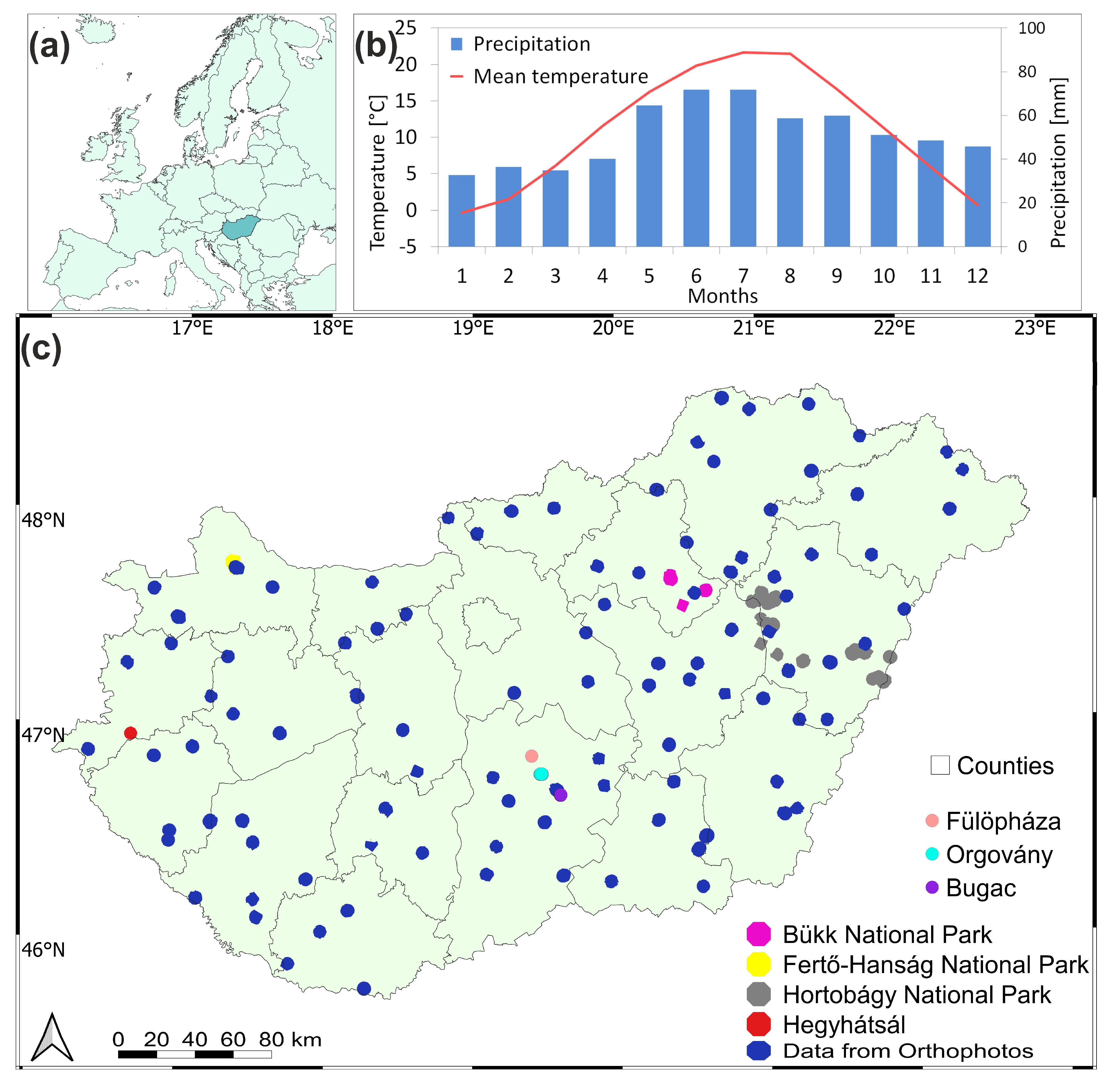
The study focuses on Hungary (with a total area of ~93,030 km²) in Central Europe (Figure 1a). The climate of Hungary is affected by continental, oceanic and Mediterranean air masses, with a long-term mean temperature of 11.1 °C (1991–2020) and mean annual precipitation of 616 mm [21] (Figure 1b). In each year of the study period (2017–2024), due to the overall warming, annual average temperatures were higher than the long-term mean, and annual precipitation sums were typically lower than 616 mm (exceptions are 2017 and 2019; see Table S1 in the Supplementary Material). 2022 and 2024 were characterized by extreme drought, especially in the eastern part of the country.

The land use in Hungary is overwhelmingly dominated by agricultural activity. According to the CORINE database [22], arable lands occupy approximately 27% of the total country area. The second most significant category is forestry; forests cover about one third of the territory. Natural grasslands and pastures are also prominent, covering roughly 16% of the land. Note that this study examined several different grassland databases in order to compare them in terms of grassland area (see Section 2.4), which means that this number is not exact but a widely used estimation. Artificial surfaces cover approximately 13%, while specialized cultivation, such as vineyards and fruit plantations, represent a smaller but distinct portion of the landscape. Finally, swamps, marshes, and natural water bodies make up roughly 4% of the total area.

2.2. Reference Datasets

First, we performed an exhaustive literature review and research (including personal communication with experimentalists) to identify possible data sources in Hungary from a variety of research teams. The target datasets included direct biomass samplings with destructive methods, and we also used forage yield data from Hungarian National Parks along with orthophoto-based bale number estimation and appropriate conversion factors. The collected grassland-related production data are mapped in Figure 1c and detailed in

Table 1. Details of collected grassland production datasets. NP means National Park.

Location	Management	Representative Area	Biomass Value	Frequency of Mowing or Sampling	Temporal Availability (Plot/Year)
					2017	2018	2019	2020	2021	2022	2023	All
Bugac (46.69° N, 19.6° E)	grazing	16 ha square	average of 78 or 156 points	three to five times a year, but only the first sampling is used	1 plot from 78 points	1 plot from 78 points	1 plot from 156 points	1 plot from 156 points				4
Fülöpháza (46.87° N, 19.42° E)	none	16 ha square	average of 16 sites	once a year	1 plot from 16 sites	1 plot from 16 sites	1 plot from 16 sites	1 plot from 16 sites	1 plot from 16 sites	1 plot from 16 sites	1 plot from 16 sites	7
Orgovány (46.78° N, 19.47° E)	none	16 ha square	average of 6 or 10 points	once a year		2 plots from 16 points						2
Bükk NP	grazing and mowing	14–158 ha	plots	most of the time once a year, if not, only the first is used	2	1	1	1	3	2	2	12
Fertő-Hanság NP	mowing	38–90 ha	plots						1		3	4
Hortobágy NP	grazing and mowing	10–112 ha	plots			6	7	9	7	26	32	87
Hegyhátsál (46.96° N, 16.65° E)	mowing	2 ha	plot		1	1						2
Bale digitalization based on orthophotos	mowing	2–67 ha	plots	one sample at different times per plot							118	118
Hungarian Central Statistical Office	grazing and mowing	525–8443 km2	20 counties	one value	20	20	20	20	20	20	20	140
Summary					25	32	30	32	32	49	176	376

. Owing to the well-known challenges of harmonizing heterogeneous grassland datasets (see Section 2.5 for details), we placed particular emphasis on the quantification of the uncertainties in the biomass samples and the inclusion of these uncertainties in the modelling framework using a Bayesian method. Furthermore, ensemble modelling was used to enhance robustness (see Section 2.7 for details).

2.2.1. Harvested Aboveground Biomass, Reference Data

We have data on harvested biomass from three areas within the Kiskunság National Park (Figure 1c, with pink, cyan and purple). In Bugac (46.69° N, 19.6° E, data from [23]), the surface coverage (%) of each plant species was recorded three times a year within 78 quadrats, 63 arranged as a 10 m resolution grid and 15 additional random positions. In 2019 and 2020, measurements were also carried out in a 30 m grid, which means 78 more measurement points. After that, the above-ground biomass was removed from the plots from a 0.1 m diameter area, then it was oven-dried for 48 h and weighed.

Although the database, which was collected in a small area with a dense grid and high temporal resolution, has great research potential, the comparison with satellite images taken at 10 m is better supported by the average biomass value representative of the area. Thus, the mean value of the first samples of each year is examined in reference to a 16-hectare square (Supplementary Material Figure S1).

Near Fülöpháza (46.87° N, 19.42° E, data from [24]) within the study area (approximately 1 km²), 16 sites were selected in 1999, eight dominated by Festuca vaginata and another eight by Stipa borysthenica, the two dominant species of sandy grasslands in the region. The percentage cover and density changes in Festuca and Stipa were visually estimated in late June or early July each year (following peak growth but before potential drought-induced dieback). Above-ground biomass was estimated from the surface areal cover (%), based on species-specific conversion factors determined through linear regression between visually estimated cover and measured biomass in a separate study at the same site [25]. Unfortunately, the sites are only characterized by one coordinate, so we use the average of the 16 sites as a centre point of a 16-hectare square around the point (Supplementary Material Figure S1).

Near Orgovány (46.78° N, 19.47° E, data from [26]) homogeneous grassland patches (ca. 5 m in diameter) were chosen that covered the variation in grassland productivity within a 1 km² area. Then one randomly located 0.5 × 0.5 m plot in each patch was sampled. Above-ground vascular plant biomass was harvested in each sampling plot at the peak of the growing season. Biomass was sorted by species, and only living material was considered in the analyses. Biomass samples were dried at 60 °C for 48 h and then weighed. Although the aim of the survey was to assess grasslands with different productivity levels, from the perspective of satellite data, they are too close to each other and thus represent a larger, inhomogeneous area covered with trees and bushes. In order to obtain a value characteristic of the landscape, we defined two 16-hectare squares around two transects of samples and averaged the measured biomass values within them (Supplementary Material Figure S1). Note that the presence of bushes and trees within squares can be a significant source of error.

2.2.2. Yield Data from Management Registers

We used mowing data originally provided in bales ha⁻¹ units from four national parks and from the plot around the eddy covariance tower at the Hegyhátsál experimental site [27]. Parcels from Bükk and Hortobágy National Park are in Eastern Hungary, near Lake Tisza (Figure 1c with magenta and grey; data source is the Directorate of Bükk and Hortobágy National Parks). Fertő-Hanság National Park is in North-Western Hungary (Figure 1c with yellow; data source is the Directorate of Fertő-Hanság National Park), just like Hegyhátsál (46.96° N, 16.65° E; Figure 1c with red). Agricultural parcel boundaries were taken from the parcel-level farmers’ claim data submitted to the Common Agricultural Policy (CAP) subsidy system in Hungary (referred to as Anonymized Database of Subsidies; data courtesy of the Hungarian State Treasury). Mowing dates and mowed bale counts came from management registers. It is common for multiple plots to be recorded with the same yield, which we tried to filter out (e.g., by merging neighbouring plots with identical yields; Figure S2a in the Supplementary Material), but this may still cause some systematic errors. Unfortunately, we were not able to fine-tune the boundaries of the plots and the unmown areas based on satellite data everywhere, but in our experience, this can only have a minor impact on the results (Figure S2b in the Supplementary Material). Yield by weight calculated using the standard value of 300 kg bale⁻¹, as proposed by the National Park or by the farmer, except for Fertő-Hanság, where data are based on precisely measured bale weight.

2.2.3. Biomass Based on Bale Digitalization Using Orthophotos

Bale numbers have been determined based on orthophotos in nearly 120 areas by the authors. The orthophotos for the year 2023 cover the entire country with a spatial resolution of 40 cm (data provided by Lechner Knowledge Centre, Budafoki u. 59., Budapest, H-1111, Hungary; Supplementary Material Figure S3a). We determined the parcel boundaries mainly based on orthophotos, but later refined them using Planet satellite images, taking into account simultaneous mowing (Supplementary Material Figure S3b,c). The size of bales was measured on stereo photos (Supplementary Material Figure S3d), then two types of bales were identified based on the dimensions. Weight was calculated based on estimates made by farmers: 300 kg bale⁻¹ for 125 cm diameter and 400 kg bale⁻¹ for 150 cm diameter. It should be noted that counting bales, the delineation of parcel boundaries, the determination of bale height, and the uniform calculation of bale weight may all contain errors that accumulate.

2.2.4. Yield Data from the Hungarian Central Statistical Office (HCSO)

The territorial statistics of the HCSO on agricultural production are based on the collection of data on actual use provided by farm organizations and individual farms according to its own methodology [28]. The methodological descriptions of data collection clearly define the concept of “grassland” in the HCSO nomenclature: only grassland that has been used for at least five years for grazing animals (pasture) or mowing (meadow), or grassland that is not used but has received support for being kept in good environmental and ecological condition, is considered grassland. The annual grass hay yields are reported by county (NUTS3 level) in tons per hectare. Note that the data were obtained through personal communication.

2.3. Remote Sensing Information

2.3.1. Copernicus LAI

LAI is an integrative measure of plant development stage as it quantifies the total leaf area per unit surface area. Higher leaf area is typically associated with larger biomass in herbaceous vegetation and can indicate larger photosynthetic capacity and biomass accumulation. This is an intrinsic canopy variable that should not depend on observation conditions. Note that vegetation LAI as estimated from remote sensing includes all the green contributors such as the understory when existing under forest canopies [29]. LAI in this study was used to adjust biomass samples that are made using machinery-based industrial mowing (considering the remaining biomass).

The Copernicus Global Land Service (CGLS) provides a collection of 300 m LAI, FPAR and Fraction of Green Vegetation Cover (FCover) [29]. These products were produced and delivered from Proba-V Vegetation (VGT) data from January 2014 to June 2020, and from the Ocean and Land Colour Instrument (OLCI) on the ESA Sentinel-3 platform since July 2020, ensuring continuity of the 300 m products. The variables are calculated globally on a 10-day basis.

2.3.2. High-Resolution Vegetation Phenology and Productivity (HR-VPP) Product

The Copernicus Land Monitoring Service (CLMS) disseminates the so-called High-Resolution Vegetation Phenology and Productivity (HR-VPP) product for Europe from 1 January 2017 onwards [30]. HR-VPP is derived from Sentinel-2 images and available at 10 m resolution. The layers of vegetation phenology and productivity parameters (VPPs) are derived from seasonal trajectories of plant phenology index (PPI) [31], since PPI was found to have the strongest relationships with photosynthetic phenology as represented by annual gross primary production (GPP) [32]. In their research, Tian et al. [32] examined the performance of NDVI, EVI2, and PPI derived from Sentinel-2 data for Europe-wide phenology mapping, and among the three parameters, they recommended the PPI for VPP derivation.

The VPPs and corresponding quality layers are generated using the Fortran version of the TIMESAT 4 software package, developed by Lund and Malmö University, for analyzing time-series of high-spatial resolution satellite sensor data [33,34]. Since all satellite images from the year are used for processing, the derived VPPs are published annually, after the end of the growing season(s).

Of the published quantities, the maximum PPI [35] and total productivity [36] (referred to as MAX PPI and TPROD, respectively) were used. Total productivity (TPROD) is the integral of PPI that is the sum of all daily PPI during the growing season. The latter (being the growing season integral computed as the sum of all daily values minus their base level value [30]) can be considered as a proxy of potential biomass accumulation. The quality flag layer provided with the VPPs was applied for preliminary filtering: only pixels with high or medium reliability (QFLAG > 6) were used. After filtering, we assigned the average of the pixels falling within the 16-hectare area to the plot, which we then compared with the measured biomass. With this averaging, we assume the plot to be homogeneous, just as in the case of biomass measurement.

Note that in HR-VPP the number of output seasons per year was limited to a maximum of two per year according to the TIMESAT logic, of which both were taken into account in this study. According to our experience, the presence and significance of the second season in our country is relatively small compared to the first season in most of the years (Supplementary Material Figures S4 and S5).

2.4. Estimation of the Spatial Extent of Grasslands in Hungary

The estimation of the grassland area of Hungary was based on different data sources. According to Belényesi et al. [16], the total grassland area identified differs largely depending on the methodology and grassland definitions. We would like to emphasize that it was out of scope of the present research to decide which database is more reliable (or realistic) when it comes to grassland areas, so below we present statistics from several different sources.

The well-known and widely used CORINE Land Cover (CLC) product offers a pan-European land cover and land use inventory with 44 thematic classes [22]. The product is updated with new status and change layers every six years—with the most recent update made in 2018, so here we computed statistics from the status layer of 2018.

The Copernicus High Resolution Layer (HRL) Grasslands maps the location and size of permanent and temporary grasslands, in addition to providing information on mowing events across Europe [37]. The grassland status layers provide a basic land cover classification with two thematic classes (grassland/non-grassland), produced yearly, and have a spatial resolution of 20 and 100 m for 2015, and 10 and 100 m from 2017 onwards.

The regional reports on agricultural activities published by the HCSO are based on data collected from agricultural organizations, individual farms, and selected individual farms [28]. Data on actual grassland use is collected using questionnaires and supplemented with data from other statistical surveys.

In Hungary, the Space Remote Sensing Department of the Lechner Knowledge Centre performs a reliable mapping of the entire territory of Hungary, which annually carries information on grasslands and agricultural areas (called National Agricultural Maps; NAGRI). One of the main objectives of mapping is the delineation of permanent grassland (i.e., areas with confirmed presence through a period of 5 years). The maps are generated at a resolution of 20 m using a random forest algorithm, Sentinel-2 satellite time series, and Sentinel-1 temporal integrals.

The National Ecosystem Map of Hungary (NECOMAP; [38,39]) was prepared to fulfil the obligations related to the European Union Biodiversity Strategy, Mapping and Assessment of Ecosystems and their Services (MAES). The map shows the spatial distribution of ecosystems in Hungary using a three-level category system in the form of a thematic raster with a spatial resolution of 20 × 20 m for the base year 2015/16.

For a detailed description of the maps mentioned, see the Supplementary Material. Note that quantification remains a major source of uncertainty in the study (that will be discussed later).

2.5. Harmonization Challenges of Multi-Source Reference Data

The compilation of a country-wide grassland biomass reference dataset inevitably involves combining highly heterogeneous data sources that differ in sampling design, spatial scale, management regime, and measurement protocols (Table 1). Point-scale destructive sampling (e.g., Bugac, Fülöpháza, Orgovány) provides high-quality, species-level information but covers limited areas. Parcel-scale management register data from National Parks rely on bale counts with standardized weight assumptions, while the orthophoto-based bale digitalization method introduces additional uncertainties related to parcel delineation, bale sizing, occasional bale removal before digitization, and conversion factors. Finally, the Hungarian Central Statistical Office (HCSO) dataset offers excellent spatial representativeness at county level but is based on aggregated farmer reporting with its own methodological specificities and uncertainties.

Major harmonization challenges include: (i) inconsistent grassland definitions and management histories across sources; (ii) differences between HAB and AGB, particularly due to stubble left after mowing; (iii) variable moisture content (air-dry vs. oven-dry biomass); (iv) incomplete documentation of grazing intensity and timing in mixed grazing-mowing systems; and (v) potential geolocation and boundary inaccuracies in parcel-based data. These issues are inherent to multi-source integration and represent a well-recognized limitation in large-scale grassland productivity studies. The large discrepancies in grassland area estimates observed in this study (Figure 2) underline the pressing need for standardized definitions and mapping protocols.

To mitigate the impact of these heterogeneities and reduce the risk that results are dominated by biases from any single data source, we adopted a Bayesian framework combined with an ensemble modelling strategy. All reference observations were grouped into three independent selections. First, the observations were split into three independent groups to establish a multi-model framework. These groups are referred to here as “Selections”. Selection No1. contains all the biomass data collected by cutting at point level or mowing in parcels. Selection No2. includes data from biomass estimation based on bale digitalization using orthophotos, and Selection No3. examines HCSO data alone as it has large spatial representativeness. We also examined the data sampled using the cutting method at specific points (Fülöpháza, Bugac, and Orgovány) separately, but since these samples were taken in areas with extremely low yields and thus the national extrapolation of the models fitted to them cannot be considered representative, we do not present them here as a separate selection group. Given that we use two satellite proxies and three independent observation data selections, a total of six models were constructed.

Combined with the two remote sensing proxies (MAX PPI and TPROD), this resulted in six independent models. The ensemble approach (detailed in Section 2.7) explicitly accounts for structural differences among data sources and provides a more robust estimate of ANPP than any individual model.

2.6. Post-Processing of Observation Data

Due to the well-recognized ambiguity of productivity [40], first the nomenclature must be set, and the methodology used to approximate ANPP must be properly described. In case of heterogeneous data sources that are used in the study, the different biomass metrics must be harmonized.

Most of the data sources detailed in Table 1 provide estimates of harvested aboveground biomass (HAB), and it is used to approximate the total aboveground biomass (AGB, including standing dead biomass; [14]). In grasslands, HAB and AGB, estimated after the intensive spring growth, are widely used to estimate ANPP, that is, aboveground net primary production. ANPP, by definition, is the growth (i.e., biomass increment) of the aboveground plant parts within a year. In our study, HAB was considered to be equal to AGB in the case of complete clipping (when all biomass is removed from the target plot). If the HAB is the result of mowing, additional considerations are needed (e.g., [41]). Grass mowing with machinery always leaves a fraction of the total biomass at the site to support regrowth (the cut part is left at the site for a few days to dry out, then it is packed into bales and removed from the site). The residue is referred to as stubble in some studies. In this sense, HAB is not equal to AGB; thus, ANPP is not approximated well.

In order to use a harmonized dataset, correction was applied to the HAB data observed in situ or estimated from other methods. Using the available LAI dataset, we estimated the change in LAI (that is considered a proxy for biomass) before and after harvest. LAI before harvest was approximated by the maximum LAI in the first half of the year. As the relatively smooth LAI dataset distorts (masks) the immediate LAI after mowing, we uniformly used LAI = 1 as an approximation for the post-harvest LAI. This is supported by ceptometer-based measurements from the Hegyhátsál grassland experimental site in Hungary (unpublished data; see [27] for site description). The change in LAI was associated with HAB, and the total LAI was used to estimate ABG. This procedure ensured the comparability of the data and the homogeneity of the entire dataset (as homogeneous as possible despite the uncertainties) that is used for model construction and upscaling. In this sense, in the Section 3, HAB always implicitly means corrected biomass observation.

As peak biomass observations are available in Hungary for the first mowing (that is, the only cut in some regions), ANPP was estimated first for this time period (typically around the beginning of June). After mowing, regrowth can fail in some regions during summer due to lack of precipitation. However, in autumn, after the occasional summer heat and drought, there is a secondary growth with typically smaller biomass production. As this secondary growth contributes to the annual ANPP, we used the relationship established based on the first cut and extrapolated it to the second one using the remote sensing data and the selected VI/biophysical variable (MAX PPI or TPROD) in the second half of the year. Annual ANPP was estimated as the sum of the two simulated AGB.

It is important to note that most of the observation-based data report air-dry biomass rather than dry matter (DM). Dry matter refers to oven-dry biomass, i.e., the mass remaining after removing its water content through heating. Consequently, the HAB and ANPP values presented here inherently include some residual water content. To maintain consistency, we intentionally report biomass in gBM (grams of biomass) and MtBM (megatons of biomass for national totals), reflecting the air-dry nature of the underlying observations. In this respect, the gBM values provided here differ from the gDM units commonly used in the literature. Establishing precise conversion factors for estimating dry matter was beyond the scope of this study. However, approximate conversion can be applied when needed (e.g., assuming a typical air-dry water content of ~14%).

2.7. Statistical Analysis

Linear models were used to establish relationships between the observation-based field evidence (HAB) and the remote sensing-based biophysical data (MAX PPI and TPROD). The observation-based, plot- and county-wise datasets were combined with three different logics to support probabilistic ensemble estimation.

Bayesian method was used to construct robust linear models and estimate the prediction uncertainties as well. The Bayesian formulation provides full posteriors over the coefficients and posterior-predictive intervals that propagate parameter uncertainty into predictions. More flexible machine-learning models (random forests, gradient boosting, neural networks) would require substantially more data to be estimated and validated reliably to avoid overfitting. The method relies on the biomass observations and their associated uncertainty. This means that uncertainty had to be estimated for each biomass sample separately. This turned out to be a challenging task. As the first approach, we used an expert guess for the uncertainty based on the biomass sampling method. However, analysis of the biomass observations and the associated remote sensing proxy data revealed that the dataset is associated with so-called epistemic uncertainty. It means that uncertainty was very low for some samples that were unrealistically low but at the same time associated with high values of TPROD and MAX PPI. This kind of contradiction might be associated with erroneous reporting of the harvested biomass by the farmers, or some unexpected or unreported bale transportation/dislocation, or any error associated with human behaviour. To tackle this issue, we selected a different approach for the uncertainty estimation that is objective and repeatable. We selected the Gaussian kernel-based method to quantify the observation errors.

In order to explicitly model heteroscedasticity, point-specific variance was calculated using Kernel Variance Estimation. The critical parameter in this method, the bandwidth, defines the size of the local neighbourhood used to estimate noise. This bandwidth (in the satellite proxy data) was strategically chosen to balance two core theoretical assumptions: local stationarity and statistical stability. Specifically, it was set as narrow as possible to ensure that variance is only estimated from biologically and environmentally similar measurements, while keeping just wide enough to capture a sufficient local sample size. Supplementary Material Figure S7 shows the variance estimates as a function of the satellite proxy. These estimates are purely data-based and objective, and can be applied in similar situations.

The six biomass models were constructed using Bayesian linear regression, taking into account the uncertainty estimations quantified based on the kernel variance estimations. It should be stressed that the choice of a Bayesian framework over classical ordinary least squares (OLS) estimation was not motivated by philosophical preference but by practical necessity. In our setting, the measurement uncertainty in biomass varies substantially across observations, meaning that the assumption of constant error variance—which is fundamental to ordinary least squares—is violated by the nature of the data itself. Prior knowledge about the error distribution at each observation point is available, and a framework capable of incorporating this information directly, rather than discarding it, was therefore required. A Bayesian approach provides exactly this: observation-specific measurement errors can be encoded directly into the likelihood, producing posterior predictive distributions that faithfully reflect the heteroscedastic structure of the data. This is important because the ultimate goal is not simply to calibrate the individual models but to apply them at national scale and combine their predictions into an ensemble. For such a combination to be meaningful, realistic uncertainty estimates are needed for each model—not the overly optimistic or poorly calibrated confidence intervals that classical methods tend to produce under violated assumptions. The Bayesian framework provides these estimates naturally, enabling principled weighting strategies where individual model contributions reflect their demonstrated predictive reliability rather than being treated as equally trustworthy.

For each model, the relationship between the predictor and biomass was specified as a linear function with an intercept and a slope. The observation error at each data point, as described above, was entered directly into the likelihood as the standard deviation of a normal distribution. This means that instead of estimating a single residual variance across all observations—as the ordinary least squares method would do—each observation carries its own measurement uncertainty into the inference, which we consider a more honest representation of the data-generating process.

Informative priors for the intercept and slope were derived from OLS. Each parameter was assigned a normal prior centred on its corresponding OLS point estimate, with a standard deviation set to three times the OLS standard error. It is acknowledged that centring priors on estimates obtained from the same data constitutes a data-informed prior specification. However, the deliberately inflated standard deviations ensure that the priors remain weakly informative and that the posterior is overwhelmingly driven by the likelihood. In practice, the choice of prior centre has negligible influence on the results—it serves only as a pragmatic anchoring point that aids convergence without constraining the inference.

Posterior distributions were estimated using the No-U-Turn Sampler (hereafter referred to as NUTS), an adaptive extension of Hamiltonian Monte Carlo that eliminates the need for manual tuning of the trajectory length. For each model, 3000 posterior samples were drawn per chain following a warm-up phase of 1000 iterations. Convergence was assessed through visual inspection of trace plots, the Gelman–Rubin R-hat statistic, and effective sample size. Posterior predictive distributions were generated for each model, and 90% credible intervals were computed for the predicted biomass values. Model comparison was performed using leave-one-out cross-validation estimated via Pareto-smoothed importance sampling (hereafter referred to as PSIS-LOO), which approximates the expected log predictive density and penalizes model complexity through out-of-sample prediction accuracy. The resulting LOO scores, together with the per-model posterior predictive uncertainties, inform the subsequent construction of the national-scale ensemble.

After calibration, the six best-fit models were not reduced to a single equation; instead, their predictions were combined into an ensemble, so that the choice among the candidate biomass–vegetation index relationships means an explicit, quantified source of uncertainty rather than a fixed assumption. For every grassland pixel and every year, each of the six models produced a full posterior predictive distribution of aboveground biomass from its corresponding vegetation index. These six distributions were then combined using weights derived from the PSIS-LOO results, so that each model contributed in proportion to its demonstrated out-of-sample predictive performance: models that predicted the held-out observations better received larger weights, and the weights were normalized to sum to one across the six models. Because the weighting acts on the entire predictive distributions and not only on the point predictions, both the parameter uncertainty and the observation-specific (heteroscedastic) uncertainty of every model are carried through into the ensemble prediction.

The national level upscaled estimate of total grassland aboveground biomass production was then obtained by repeated Monte Carlo sampling. In each iteration, one of the six models was drawn at random with probability equal to its ensemble weight, a biomass value was sampled from that model’s posterior predictive distribution at each grassland pixel, and the pixel values were summed over the national grassland mask to produce one realization of the country-level total. Repeating this many times yielded the full distribution of national production, from which we report the median and the 90% credible interval. Two independent sources of uncertainty were propagated through this procedure. The first is the uncertainty in the biomass–index relationship itself, represented by the ensemble of six models together with their posteriors, so that no single reference equation is assumed to be correct. The second is the uncertainty of grassland area selection, which was propagated by repeating the spatial aggregation over the alternative grassland delineations within the same Monte Carlo loop. The complete workflow was run separately for each year of the study period, and the resulting year-to-year differences—each accompanied by its own credible interval—constitute the reported interannual variability of grassland production.

Table 2. Technical details on the applied model construction procedure.

Item	Value
Likelihood	yi ~ Normal (α + β·xi, σi), σi fixed per observation
Prior—intercept	Normal (α^_OLS, (3·SE_α)2)
Prior—slope	Normal (β^_OLS, (3·SE_β)2)
Sampler	No-U-Turn Sampler (NUTS)
Chains	4
Draws/tuning per chain	3000/1000
Posterior samples per model	12,000
Convergence criterion	R-hat = 1.00 (all parameters)
Model comparison	PSIS-LOO
Observations per Selection (1/2/3)	117/118/140
Software	PyMC 5.28.1, ArviZ 0.23.4, statsmodels 0.14.6, Python 3.12.3
Ensemble weighting	Equal; law-of-total-variance decomposition

provides information about the software packages used and technical details to support repeatability.

3. Results

3.1. Grassland Area Estimation

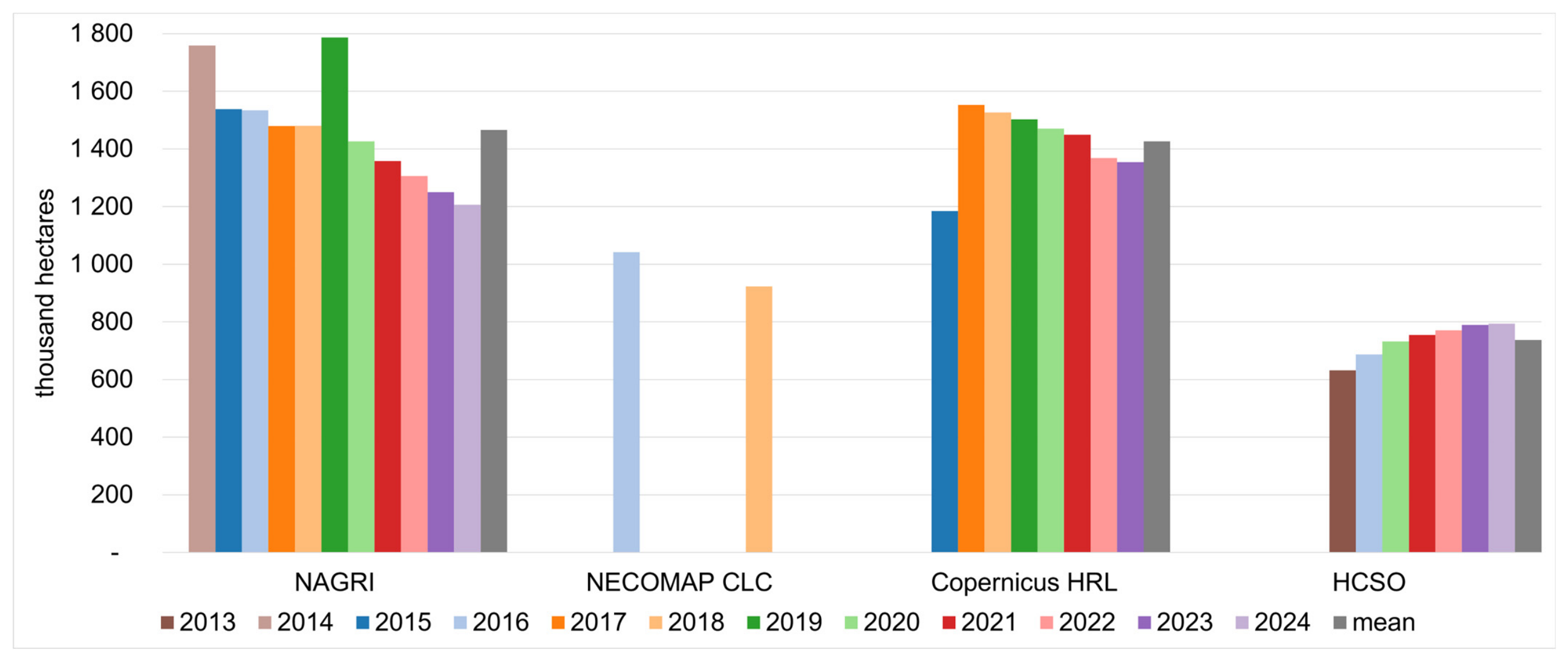
Figure 2 summarizes the grassland area estimations for the whole country, calculated from the spatially explicit datasets detailed in the Supplementary Material. The figure clearly shows that there is a large variability between the estimations.

The highest grassland area was identified by Copernicus HRL, covering ~1.35 million hectares in 2023, which is roughly 14.5% of the country’s territory. The variability between the years shows that the total area of grasslands is decreasing. The decrease between 2017 and 2023 is 198,550 hectares, which represents nearly 13% of the grasslands in 2017. NAGRI also shows a steady decline in total grassland area (2019 was an exception), as it decreased by 15.8% (222,000 hectares) between 2015 and 2024. The difference between the years might be associated with classification errors to some extent. The NECOMAP mapped 25% less grassland than the corresponding NAGRI data. The CLC for 2018 provides an even smaller area, with less than 1 million hectares. In this dataset, the spatial resolution might restrict some additional grassland mapping. The smallest grassland area (about 50% of Copernicus HRL or NAGRI) is estimated by HCSO statistics, and the trend shows an increase in grassland territory. The reason for this is likely the applied definition of grassland, as explained in detail in the Supplementary Material. Supplementary Material Figure S6 shows an example to demonstrate the differences between the grassland categories in the databases we used.

Based on multi-year averages where data were available, the total grassland area varies significantly across sources: Copernicus HRL reports the highest coverage at 1,426,229 ha, followed by NAGRI (1,317,885 ha), NECOMAP (1,041,958 ha), CLC (923,340 ha), and HCSO (754,720 ha). The difference between the minimum and maximum multiannual average is 671,509 ha.

3.2. Relationship Between Observation-Based and Remote Sensing Data

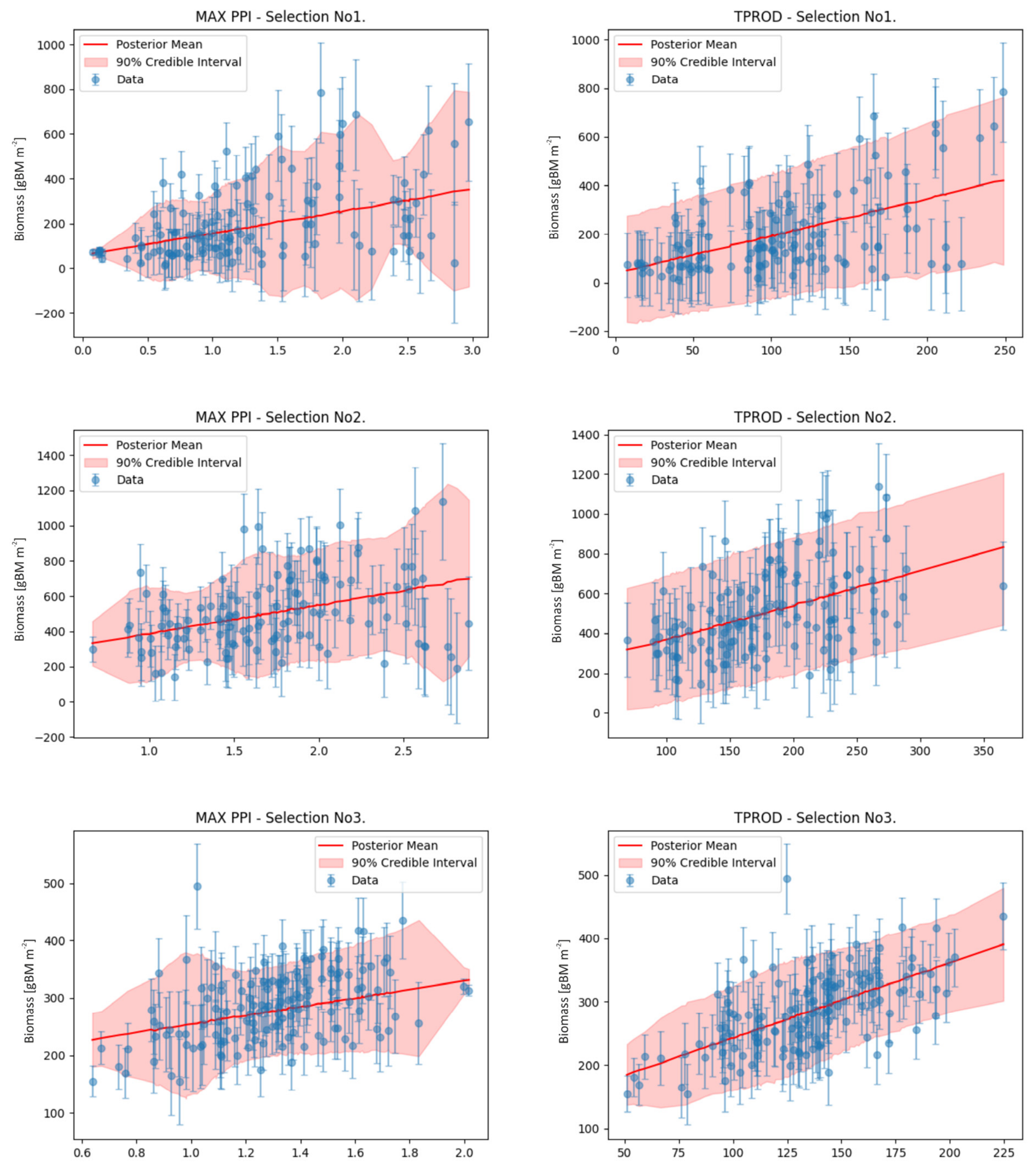
Biomass data from all three data selections (No1., No2. and No3.) were plotted against parameters from the HR-VPP database (MAX PPI and TPROD; Figure 3), and models were constructed using a Bayesian framework. The resulting models are shown in Figure 3 together with the 90% credible interval of the fit. Uncertainty of the observations is also indicated. Since there is no uniform number of samples available for each year, it is not feasible to examine each year separately; the data for each year were handled together.

It is clear from the plots that the HAB values remain below 1200 gBM m² in all cases, and the data derived from orthophoto digitization (Selection No2.) have the largest variability. The fitted regression equations are summarized in

Table 3. Fitted regression equations that establish the relationship between the satellite-based proxies and the reference biomass data. In all cases, x represents the remote sensing proxy data. No1., No2., and No3. represent the different observation data selection logic described above. The numbers below the equations represent the 3rd and 97th percentile intervals of the slope and intercept, respectively.

	MAX PPI	TPROD
Selection No. 1.	97.80x + 58.52	1.54x + 37.97
	76.58–117.45	1.11–1.97
	47.84–68.85	−10.38–86.24
Selection No. 2.	164.00x + 222.64	1.73x + 194.36
	105.94–219.69	1.18–2.31
	136.15–320.32	880.05–299.53
Selection No. 3.	75.60x + 178.82	1.18x + 124.51
	58.38–91.50	0.99–1.35
	154.22–203.57	100.20–150.51

. We also report the uncertainty of the fitted models by presenting the 3rd and 97th percentile of the derived slope and intercept values. Note that the slope and intercept values are not comparable due to the markedly different magnitudes of the satellite proxies (MAX PPI ranges between 0 and 3, while TPROD varies between 0 and 400).

As the next step, we used the presented 6 equations to upscale the observations to the country level. In the case of negative modelled HAB (which is the byproduct of the fitting using noisy data), we set HAB to zero, which is a common practice in ecological modelling. This can theoretically affect the results, but given the fact that such low production is rare in the country, the effect of this adjustment is negligible.

3.3. Country-Level HAB and ANPP

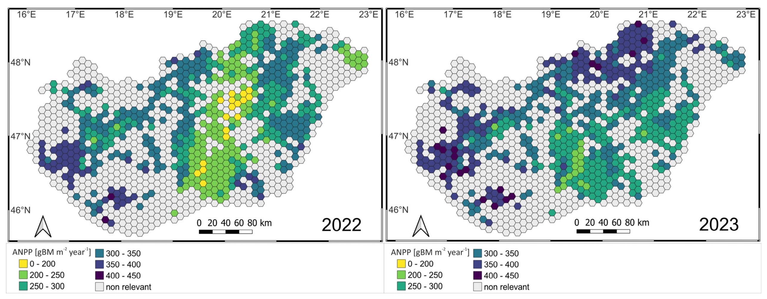
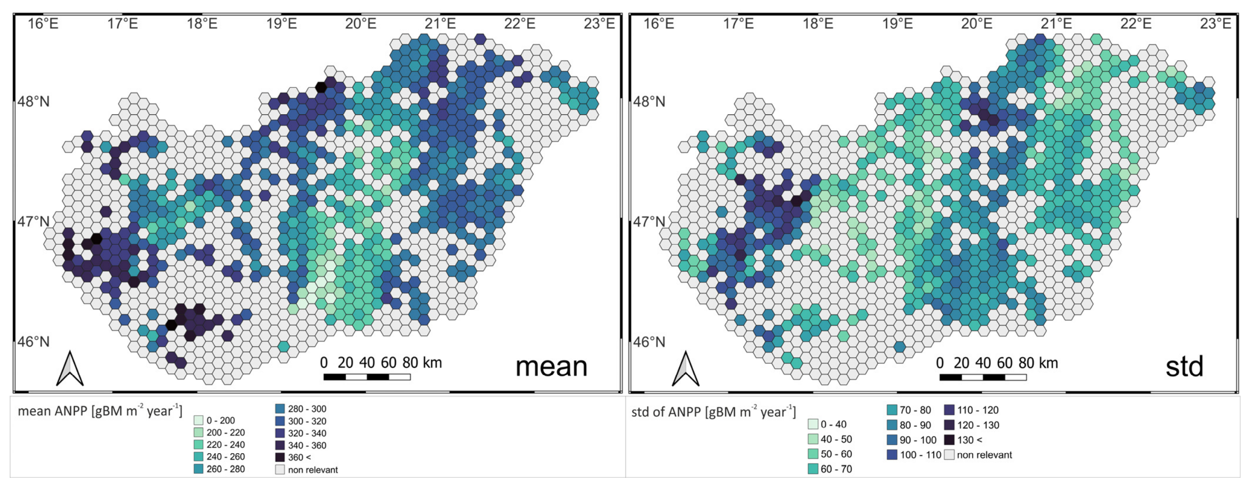
The six equations presented above were used to derive national mean HAB for each year, but only one of them (the one based on Copernicus HRL against TPROD with Selection No3. reference data) is presented here as maps for two extreme years (Figure 4), as well as the average and standard deviation between years (Figure 5). Supplementary Material Figure S8 shows maps for all examined years from 2017 to 2024.

The results were produced at a spatial resolution of 10 m, and integration into hexagons with a diagonal length of 10 km was performed solely for visualization purposes. Note that we coloured all hexagons where the proportion of grassland was at least 10% (Supplementary Material Figure S9 shows grassland proportion relative to the area of hexagons), but obviously only grassland pixels were taken into account in the spatial aggregation. When deriving average yields and later country totals, we always used 10 m resolution. In all cases, the maps represent the sum of the two seasons, i.e., the yield (ANPP) for the entire year.

The aggregated maps for 2022 and 2023 show a difference in ANPP between an extremely dry year and a year with higher precipitation (Figure 4). In both years, yields in the driest areas were less than 200 gBM m⁻² (Figure 4, yellow colour). The minimum value of ANPP in 2022 was 125 gBM m⁻², and there are only two hexagons where it exceeds 400 gBM m⁻². In 2023, the minimum of the area mean ANPP values is below 250 gBM m⁻², but in many cases exceeds 400 gBM m⁻².

The long-term average ANPP map shows that the central, lowland, and sand ridge areas of the country have lower average yields, while the western and northeastern hilly and mountainous regions have higher average yields (Figure 5, left plot). The long-term standard deviation of ANPP (i.e., the interannual variability (IAV) of ANPP) characterizes each area in terms of stability of annual production. It is interesting to note that the spatial correlation between the mean and the standard deviation is non-significant, meaning that there is no relationship between mean biomass production and its temporal stability. IAV is the smallest in the Central and northern part of the country. The largest IAV is present in the western part of Hungary (Dunántúl) and the northern hilly region.

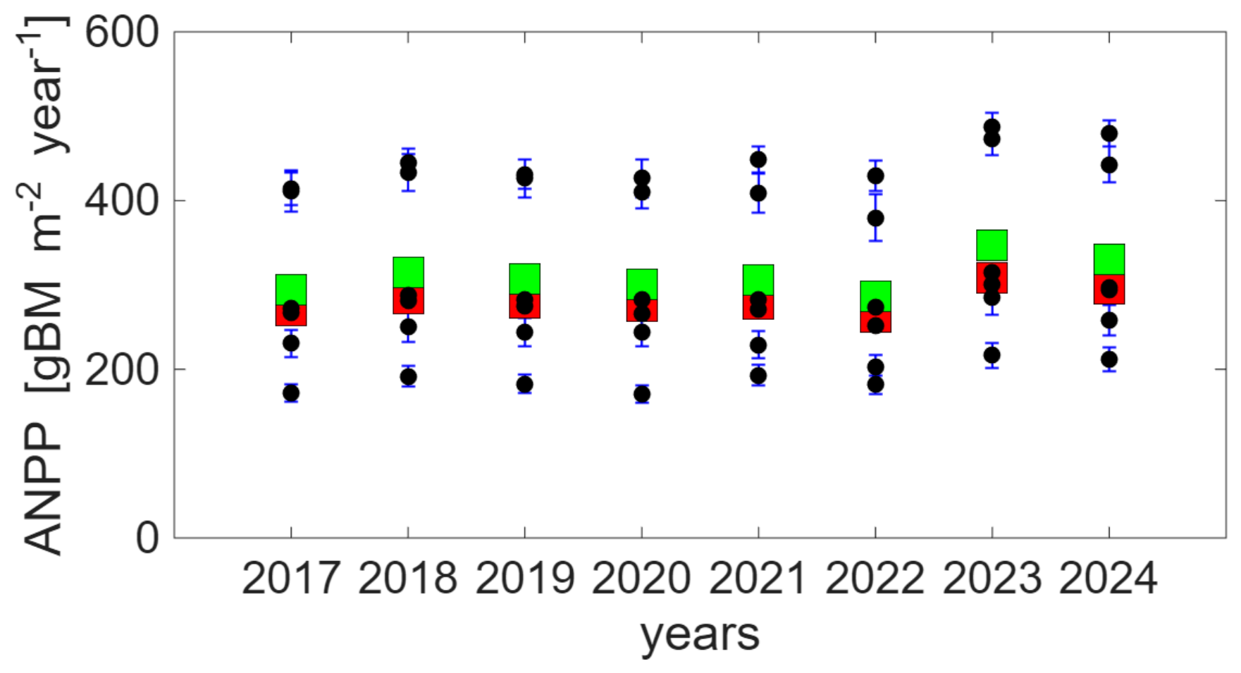
In this study, the mean values are used as the representative, ensemble-based estimation of ANPP. The mean ANPP calculated from all models and multiannual means are shown in

Table 4. The country-wide mean ANPP estimates. Data are shown for the individual years and also for the multiannual means. All units are given in gBM m⁻². The predictor means the satellite proxy, while obs represents the reference data selection group.

		2017	2018	2019	2020	2021	2022	2023	2024	Mean
MAX PPI	No1.	172.29	191.40	182.77	170.66	193.09	181.76	216.73	211.60	190.04
MAX PPI	No2.	413.44	445.48	431.01	410.70	448.31	429.32	487.96	479.35	443.20
MAX PPI	No3.	266.77	281.54	274.86	265.51	282.84	274.09	301.12	297.15	280.48
TPROD	No1.	230.73	249.99	244.00	244.21	229.02	202.61	285.42	258.66	243.08
TPROD	No2.	411.27	432.94	426.21	426.44	409.35	379.63	472.81	442.70	425.17
TPROD	No3.	272.71	287.52	282.92	283.08	271.40	251.09	314.76	294.18	282.21
	mean	294.53	314.81	306.96	300.10	305.67	286.42	346.47	330.61	310.70
	median	269.74	284.53	278.89	274.29	277.12	262.59	307.94	295.67	281.34

. The large difference between 2022 and 2023 is most evident in the case of model No2. Based on TPROD, there is a difference of 93.2 gBM m² between the average yields for the two years. Using the estimates of all models, the mean of the multiannual grass yield in Hungary is 310.7 ± 19 gBM m⁻² (the median is 281.3 gBM m⁻²). Uncertainty is calculated with error propagation rules based on the independent estimations. It is interesting to mention that the overall mean of all observations is 328.6 gBM m⁻², which means that the collected in situ data can be considered representative of the whole country.

The individual ANPP time series (from 2017 to 2024; see Figure 6) estimated by the different proxy-data selection combinations were compared with the time series of the annual means and medians to propose possibly one single method that approaches the ensemble relatively well. Considering the mean time series, the TPROD–Selection No3. combination (bias ≈ −28.5 gBM m⁻², R² = 0.87) and also the MAX PPI–Selection No3. (bias ≈ 30.2 gBM m⁻², R² = 0.81) seem to be suitable to represent the robust estimation if bias is the main criterion. Note that all time series show similarly high R² values (0.81–0.87).

Using the average annual yields (Figure 6) and the grassland area calculated based on various grassland databases (Figure 2), national grassland yield totals were obtained (

Table 5. The country-wide mean and standard deviation (std) of total ANPP (averaged for all years) based on the different combinations of observation selections, satellite proxies, and grassland databases. std in the last column represents the uncertainty associated with the method selection, for a given grassland area database. std in the last row represents the uncertainty associated with the grassland area selection for a given ANPP estimation model. All units are given in Mt year⁻¹.

	MAX PPI 1	MAX PPI 2	MAX PPI 3	TPROD 1	TPROD 2	TPROD 3	Std
CLC	16.74	39.00	24.67	21.05	37.01	24.56	8.90
NAGRI	24.83	58.00	36.74	31.87	55.79	37.03	13.31
Copernicus HRL	26.04	60.86	38.17	34.07	59.28	43.39	13.94
HCSO	14.07	32.78	20.73	17.96	31.39	20.84	7.50
NECOMAP	23.01	53.70	34.00	29.10	51.15	33.94	12.28
std	5.25	12.32	7.73	6.99	12.13	9.20

). If we use each data selection–grassland area database combination as an individual estimation, the annual means vary between 14.1 and 60.9 Mt year⁻¹. The multiannual mean is 34.3 ± 13.3 Mt year⁻¹ (median is 33.4 Mt year⁻¹), which is the result of the ensemble approach, and is considered the best estimate in this study. The uncertainty is simply calculated as the standard deviation of all estimations, with multiannual means.

We examined whether it is the grassland area estimation or the model construction that has a larger influence on the country totals. Using multiannual mean ANPP data, Table 5 shows that the standard deviation of the results that are caused by the grassland area estimation varies between 5.3 and 12.3 Mt year⁻¹ (the mean is 8.9 Mt year⁻¹), while it ranges between 7.5 and 13.9 Mt year⁻¹ (the mean is 11.2 Mt year⁻¹) that is the uncertainty associated with the model selection method (considering only a single grassland area database). The results indicate that, within the frame of the present study, the remote sensing-based linear model selection has a larger influence on the country totals than the grassland area database selection.

The country total ANPP time series (i.e., 8 years of ANPP), using all 30 individual estimations for the different satellite proxy–data selection–grassland area combinations (Table 5), were compared with the annually calculated means to propose a single method that best represents the ensemble time series. Using the mean of the 30 individual estimations for the country totals per year, the Copernicus HRL–TPROD Selection No1. combination was associated with the smallest systematic error (bias = −0.2 Mt year⁻¹, R² = 0.83). Bias was similarly very low (−0.3 Mt year⁻¹) for NECOMAP–MAX PPI Selection No3. and NECOMAP–TPROD Selection No3. with R² = 0.57 and 0.86, respectively.

If we combine the results from the country-mean, unit area-based ANPP and the country total biomass production in the context of representative method selection, and select the median as the proposed approach calculation method for the ensemble estimation in both cases, the NECOMAP-TPROD-Sel. No3. combination seems to be an optimal choice. This is our proposed modelling approach for generic studies at small scales or even at the country level.

To explore the weather effects on interannual ANPP variability, annual ANPP estimates were correlated with monthly meteorological variables over the 2017–2024 period. Owing to the limited length of the time series (n = 8 years), the analysis should be regarded as exploratory.

The strongest relationship was found with mean air temperature in September (R = 0.91 for the ensemble mean ANPP), while vapour pressure deficit in September (VPD) also showed a strong positive association (R = 0.82; p < 0.01). Similar relationships were observed for the national total ANPP estimates, with significant positive correlations for September VPD (R = 0.89) and marginally significant correlations for September mean temperature (R = 0.83; p < 0.01), whereas September precipitation exhibited a negative relationship (R = −0.83; p < 0.01). In contrast, no significant relationship was found with summer precipitation.

These results do not necessarily imply a direct causal effect of September meteorological conditions on annual grassland productivity. Rather, September climate variables likely reflect the overall hydroclimatic character of individual years and also indicators of the conditions of secondary autumn regrowth of grasslands in Hungary after the summer drought and senescence. For example, the exceptionally dry year 2022 was characterized by substantially reduced ANPP, whereas the favourable climatic conditions of 2023 coincided with a strong recovery in grassland productivity. Longer time series will be required to disentangle the relative effects of temperature, precipitation, and drought on interannual ANPP variability, also taking into account legacy effects from previous climate anomalies.

4. Discussion

4.1. Grassland Area Estimations

The first and perhaps the most complex issue of grassland mapping is the definition of grassland itself. There are so many heterogeneous and diverse grassland types worldwide that it is not easy to come up with a general definition [17]. This difficulty is further complicated by the dynamic variability of grasslands within a year, as well as the transition between grasslands and croplands or wooded/forested areas or wetlands between years. This variability can be caused by natural factors (climate, water supply, erosion, wildfires) and/or human intervention (grazing, mowing, irrigation, fertilization, sowing, cultivation). In other words, the natural and anthropogenic influences interact, and thus the grassland definition must deal with at least one of these factors (introducing the issue of distinguishing between land cover and land use). These factors demonstrate how complex it is to create a spatially explicit database that can characterize grasslands from all aspects.

At the national level within Europe, there is a distinct lack of integrated grassland inventories designed to simultaneously support nature conservation objectives and the strategic planning of grassland utilization and management. Recent assessments confirm that only a limited number of European initiatives explicitly target the mapping of grassland area and condition [16]. A compilation of European best practices for grassland mapping is currently underway within the LIFE IP GRASSLAND-HU project [42]. Several Member States have already launched substantial efforts. In Slovakia, extensive field sampling was first conducted at 20,000 sites [43,44] followed by the publication of a detailed national ecosystem map [45]. In Romania, surveys from 21,685 quadrats were used to construct the Romanian Grassland Database [46]. In the Baltic states (Estonia, Latvia, and Lithuania), a coordinated project initiated in 2014 assessed biodiversity and ecosystem services across 465,600 ha of grasslands [47]. Some of the most advanced approaches are found in the Czech Republic, where an annually updated national database covers all areas of environmental value [48,49], and in Ireland, where a national, high-resolution land-cover map was produced through an interdisciplinary collaboration [50,51].

In Hungary, there is currently no national-level, spatially explicit database providing comprehensive information on the location, extent, type, ecological status, and utilization of grasslands and grassy habitats [16]. Such a dataset would be highly valuable for ecologists and nature conservation experts, as well as for agricultural professionals involved in livestock farming and feed production [52]. The mapping method based on the General National Habitat Classification System (ÁNÉR; [53]) would be suitable for the high-precision mapping and classification of Hungarian grasslands, but it requires intensive fieldwork, making nationwide implementation extremely time-consuming and costly. This method is used to produce habitat maps for the National Biodiversity Monitoring System in 5 × 5 km² every 10 years (NBmR; [54]), as well as for mapping Natura 2000 sites, which cover approximately 21% of the country. It was also applied between 2003 and 2006 to create the Hungarian Habitat Map Database (MÉTA; [55,56]), which covers the entire country. However, the mapping units were based not on actual land-cover or habitat boundaries but on 35-ha hexagons (“MÉTA” hexagons).

In 2022, the Grassland Management Working Group of the Hungarian Livestock Breeders Association and the National Chamber of Agriculture conducted a sample-based field survey in several locations across the country to assess grassland conditions, structured around livestock feeding considerations [57]. Experts carried out fieldwork across approximately 20,000 ha in various regions. In addition, information on an additional 88,404 ha was collected through questionnaires, which gathered data on grassland size and yield, bulk fodder production, grassland management practices, mowing frequency, grazing methods, rotation numbers, grazing duration, livestock species and numbers, and the use of Ivermectin. Altogether, these grasslands represent 11.5% of the total grassland area in Hungary [57].

Among the available spatial databases at the national level, refs. [16,52] provide detailed overviews of their heterogeneity in terms of information content, mapping objectives and methodology, and accessibility. Differences among these maps arise from varying (i) mapping objectives, (ii) definitions of grassland, (iii) grassland typologies, (iv) data-production methodologies, (v) spatial resolutions, and (vi) temporal resolutions and update frequencies (see Table S3 in the Supplementary Material for details). The comparative study of Hungarian grassland extent presented in [16] covers seven databases for the year 2016 (Figure 6 in [16]).

In the current study, we used some of the datasets presented in [16], and extended the comparison for all available years between 2015 and 2024, while also including two additional European datasets (CLC and Copernicus HRL Grasslands). As shown in the Section 3, the mapped grassland area shows high variability (Section 3.1 and Figure 2), which in our case can also be attributed to the methodological differences listed above.

Clearly, the standardization of grassland definitions, typology, and mapping methodologies is a necessary next step both in Hungary and across the European Union. For example, set-aside areas may be classified as either grassland or cropland depending on the definitions and methodologies applied. Inconsistent approaches can lead to double-counting or omission. Ultimately, the entire territory must be mapped consistently, and unmapped or overlapping areas must be avoided. This is an important challenge for the coming years.

Such harmonization is essential not only for consistent biomass upscaling and productivity assessments but also for reliable reporting under the Common Agricultural Policy (CAP), Natura 2000, and national greenhouse-gas inventory frameworks. In this context, ongoing European initiatives provide promising pathways toward convergence. The LIFE IP GRASSLAND-HU project, for example, is developing integrated approaches for the long-term preservation and monitoring of Pannonian grasslands, including improved mapping methodologies that combine remote sensing with field validation to reduce ambiguities in grassland delineation and classification [42]. Similar national-level inventories in Slovakia, Romania, and the Baltic states contribute to this broader effort.

We argue that the establishment of a harmonized European grassland cadastre, with agreed definitions of permanent versus temporary grasslands, clear inclusion/exclusion criteria for shrub–grass mosaics and set-aside areas, and consistent update frequencies, should be prioritized in the coming years. Such standardization would substantially reduce current uncertainties in grassland area estimation and greatly enhance the reliability of productivity assessments such as the one presented here.

4.2. Reference Productivity Datasets for Model Construction

Communicating grassland productivity is not straightforward despite the apparent simplicity of the term “biomass” or “biomass production”. Several studies discussed the terminologies and measurement techniques that aimed to estimate some aspects of grassland productivity [14,58]. The simplest and most popular method is the destructive sampling of smaller or larger plots (with clipping) and quantifying the dry biomass and/or its carbon equivalent. HAB can approximate the total AGB (including standing dead biomass) or can only approximate some percent of it due to the remaining residue. Some methods differentiate between recently dead biomass (standing dead plants) and old dead biomass, which complicates the quantification [14]. HAB and AGB, estimated as peak biomass, are widely used to estimate ANPP. ANPP, by definition, is the growth (i.e., biomass increment) of the aboveground plant parts within a year. Herbivory, exudation and other processes can modulate ANPP, but generally HAB or AGB is a good proxy for ANPP, especially in temperate steppe grasslands [59,60]. ANPP can be expressed as dry matter or carbon equivalent, depending on the research aim.

Note that destructive sampling obviously modifies productivity and grassland functioning, as disturbance (i.e., the removal of the cut biomass) changes allocation patterns and results in ANPP that is different from the undisturbed grassland. It is fair to state that the productivity of mowed grasslands represents mowed grasslands only, and not grasslands with other management like grazing or intact ecosystems. It would be highly beneficial to standardize the sampling protocols and initiate consistent and representative sampling of biomass, supported by remote sensing data and studies like the present one.

In this study, a novel compilation of reference data was presented to support country-average ANPP. Given the heterogeneous quality of the data, uncertainties are obviously present. Nevertheless, the dataset can be used for further studies to build improved models and to clarify spatial and temporal differences in biomass production. The collected biomass data are comparable to those presented in [52] where the mean ANPP ranged between 112 and 376 gBM m⁻² between 2010 and 2014 (this study reported data between 235 and 470 gBM m⁻²). It is notable that the reference dataset derived from the farmers’ yield logs shows unrealistically low values, which means that communication and clarification of the data collection methods are highly needed. As in the study, we used the median of the ensemble; this possible underestimation does not bias the results but contributes to the uncertainty. Alternatively, strict quality control is recommended that starts in the field and ends in the reported yields to avoid biased results.

4.3. Remote Sensing-Based Upscaling of Grassland Production

Several studies have examined the relationship between multispectral satellite data and field-based measurements of grassland biomass production (see [17] for a comprehensive review). The majority of these studies rely on vegetation indices or satellite-derived products specifically designed for vegetation monitoring. With respect to modelling this relationship, both mathematical approaches (using linear or non-linear formulations) and machine learning methods have been shown to yield satisfactory results.

Ref. [61] used MODIS PSNnet to estimate AGB over a large (192,512 km²) Chinese arid and semi-arid temperate continental monsoon region. They used a significant amount of in situ measurements from 2005 to 2012, establishing their models using 975 sites and validating them using 230 sites. This study examined multiple mathematical approaches, but the unitary linear method was found to be the most accurate one with an R² of 0.55, an RMSE of 26.67 g m² and a precision of 0.69%.

NDVI and derived biophysical variables (LAI and FCover) were used to estimate biomass in [62] on a western French study area, comparing SPOT products to field measurements from 37 sites. According to their results, using linear regression, R² was 0.68 in the case of LAI, while field data showed weaker correlation with NDVI (R² = 0.3) and FCover (R² = 0.5).

In [63], five MODIS vegetation indices (NDVI, EVI2, SAVI, MSAVI, OSAVI) and two raw multispectral bands (RED and NIR) were used to estimate biomass production of Irish grasslands. Their method was applied in two study areas with a total area of 171.3 ha, in two temporal ranges (2001–2012, 2001–2005). Besides multiple linear regression, an artificial neural network and adaptive neuro-fuzzy inference system (ANFIS) were also applied to investigate the efficiency of the machine learning approach. The ANFIS algorithm performed the highest R² (0.85 and 0.76) and the lowest RMSE (11.07 and 15.35 kg DM ha⁻¹ day⁻¹) on both study areas.

Ref. [64] used a radiative transfer model called PROSAILH to calculate LAI and DM content of grasslands from Landsat 8 data. The result of LAI × DM was regarded as the estimated aboveground biomass. The method was tested on a study area covering 29,600 km² located in Qinghai Province, China. Considering ground truth data, a total of 135 30 × 30 m plots were sampled in 2014 and 2015. The results of the linear regression showed an R² of 0.64 and RMSE of 42.67 g m⁻².

The study of [65] was conducted on a natural grassland with an area of 23 ha, located in the Brazilian Pampa. The results showed the maximum R² of 0.61 for linear regression between Sentinel-2 reflectance bands and the 57 samples collected in the field. In this study, simple linear models were constructed to approximate HAB and ANPP at large spatial scales, with 10 m spatial resolution, based on MAX LAI, MAX PPI and TPROD. The R² values were moderate (spanning from 0.11 to 0.41), which can be explained by the diversity of the datasets, grassland spectral properties affected by biodiversity and the large spatial scale that the study aimed to explore. Also, as the remote sensing proxy data behaved differently, their biophysical meaning and limited information content also contributed to the uncertainty.

The comparison of the works [61,63] shows that using the same remote sensing data (MODIS) for smaller regions, better models can be constructed. However, collecting an adequate amount of field data with a balanced spatial distribution can also lead to satisfactory results on a larger scale [64].

Obviously, more complicated methods are available in the literature for the estimation of biomass and ANPP using remote sensing and in situ observations [17]. In our case, the selection of a linear method is justified by the fact that we aimed to understand the effect of the selection of the driving remote sensing dataset on the applicability as a predictor. Since there is no similar previous study for Hungary to the knowledge of the authors, this first yet simple method is fully supported. Forthcoming studies can focus on more complex methods like machine learning, XGBoost and others that could possibly provide refined estimates, but this was out of scope of the present study.

The results indicate that the remote sensing-based grassland mapping and the model selection (i.e., model construction based on in situ data selection and driving remote sensing-based proxy selection) jointly modulate the results. This clearly calls for a harmonized definition of grasslands in Hungary and in the European Union and the construction of a grassland cadastre/register database that supports policy, environmental protection initiatives and animal husbandry [16,52]. Also, critical analysis of the training data is essential. The presented ensemble approach, which is still rare in the literature, turned out to be highly useful in terms of calculating ANPP as bias-free as possible despite the obvious uncertainties and methodological difficulties.

In a wider context, other variables need to be included in the analysis. Clearly, remote sensing data are affected by the soil conditions, especially in open grasslands that occupy relatively large areas in Hungary. Topography, soil water content, species distribution and other information can supplement future studies.

4.4. Limitations of the Study

There are several uncertainties and limitations associated with the present study. These uncertainties affect all three main topics addressed here: grassland area estimation, in situ observations and remote sensing-based upscaling.

In terms of grassland identification, Section 4.1 provided a detailed overview of the uncertainties associated with international mapping initiatives. Spatial and statistical accuracy depend significantly on the original purpose of the mapping and the spatial resolution. Input reference data, satellite data, classification, post-processing, masking, and visual interpretation can all introduce errors [16]. EU-level initiatives may help resolve part of these issues, thereby constraining grassland area estimates and supporting the scientific community.

Reference data heterogeneity is another major source of uncertainty. As described in Section 2.5, the ground observations originate from markedly different protocols and spatial scales. Point-scale destructive sampling provides detailed but spatially limited information, whereas parcel- and county-scale data introduce aggregation effects and variable levels of documentation. Grazing intensity could not be quantitatively corrected due to insufficient metadata on stocking rates and timing. These issues represent a fundamental challenge in large-scale grassland studies and are the main reason for adopting the ensemble approach described in Section 2.7. Although harmonization and post-processing procedures were applied (Section 2.5 and Section 2.6), including sensitivity analyses (e.g., the post-mowing LAI assumption), some residual systematic errors inevitably remain. Future work should therefore focus on establishing a more standardized national grassland monitoring network with consistent protocols.

At the same time, due to practical considerations, we believe that it is virtually impossible to collect a large number of grassland biomass data using a completely uniform protocol for an entire country. Even if this standardization and systematic sampling could be accomplished, it would be a wrong decision to ignore existing biomass data as they contain highly valuable information on the local conditions even if the estimates have inherent uncertainties. It means that even if the most careful protocol is established and the demanding in situ field sampling is performed, uncertainties will remain and call for a mathematical solution. The presented Bayesian framework, handling heteroscedasticity and using an ensemble framework, is a mathematically sound solution to all issues mentioned; thus, the present work provides a solution for other countries and initiatives.

Considering the reference data more broadly, as mentioned above, biomass sampling was performed using markedly diverse methods. One limitation is the typically undocumented destructive sampling methodology. In the case of Fülöpháza, Orgovány and Bugac, measurements were consistently planned and accurately documented, with quantities expressed in gBM m⁻². In contrast, national park datasets rely on estimated bale numbers and uniform bale weights, which introduce additional uncertainty. HCSO yield estimates, expressed in tons per hectare unit and assigned homogeneously at the NUTS3 level, can lead to significant errors when projected onto square-metre scales. Biomass sampling must thus be further developed using standardized, well-documented methods that ensure spatial representativeness and capture within-pixel heterogeneity, ideally supported by remote sensing (i.e., a priori use of satellite data combined with a posteriori model construction). All major grassland types should be sampled, and the field surveys should be spatially well distributed.

In situ data also have limited representativeness and are inevitably affected by microtopography, soil texture, soil organic matter content, soil hydrology, occasional groundwater presence, herbivory and other undetectable processes. In some cases, multiple measurements are averaged and assigned to an arbitrarily defined square assumed to represent the landscape, thereby homogenizing small-scale differences and reducing accuracy. These uncertainties nonetheless hold valuable information. We suggest two directions for future work. On the one hand, where densely gridded biomass data exist (e.g., Bugac), repeat the modelling at the sub-parcel level using higher-resolution satellite data (e.g., Planet) and compare with the national-scale estimates. On the other hand, targeted analyses (e.g., correlation analysis) should be conducted to quantify how factors such as topography, soil, groundwater, and grazing modify biomass, and to estimate the error introduced when these factors are neglected in national extrapolations.

In Hungary, widespread annual mowing minimizes the risk of leaving “old” standing dead biomass in the field [14]. Litter, however, has its own decomposition dynamics, and its age is difficult to estimate. Dynamic models like Biome-BGCMuSo, PaSim, ORCHIDEE or ModVege are needed to quantify litter dynamics, and litter measurements should complement biomass sampling.

Moisture content is another source of uncertainty, as it is often unrecorded. Some biomass samples are oven-dried, whereas baled biomass dries naturally to an air-dry moisture content that is not exactly known. Data collection should thus be accompanied by detailed documentation of all observational data.

We assumed that post-mowing LAI approaches 1 across Hungary. This approximation is reasonable given the machinery used at Hegyhátsál, but it remains a limitation. For illustration, we recalculated ANPP using post-harvest LAI values of 0.8 and 1.2 (±20%). Based on NAGRI and a subset of observations, LAI = 0.8 reduced national ANPP by 8.1%, whereas LAI = 1.2 increased it by 4.2%. Dedicated data-collection campaigns in representative mown parcels are needed to establish a more robust threshold. Besides all mentioned uncertainties, the close agreement between the overall mean of in situ observations (328.6 gBM m⁻²) and the final ensemble mean (310.7 gBM m⁻²) further supports the representativeness of the compiled dataset despite its inherent heterogeneity.

Remote sensing-based information introduces another source of uncertainty. In mowing data, inaccuracies in plot boundaries and mixed edge pixels can slightly but measurably affect plot-level satellite proxies. More substantial errors arise from within-parcel inhomogeneity, unmown strips, isolated trees or bushes, and mosaics with wetlands. A precisely defined national grassland register, also recommended in [16], would greatly reduce uncertainties related to parcel boundaries.

Perhaps the most critical source of error is the impact of grazing on the combination of observations and satellite data, and thus on biomass estimates. The Fülöpháza dataset comes from an undisturbed area without mowing or grazing. In the national parks, Fertő-Hanság plots are mown, while in Hortobágy grazing often accompanies mowing. Even when grazing presence is known, its timing and intensity are usually undocumented, preventing explicit correction. Some of this limitation can be mitigated through precise visual interpretation, which we applied in several cases using orthophotos, as well as sub-parcel mowing data that may be available from precision-agriculture providers.

Finally, the remote-sensing time series is heavily filtered and smoothed, which effectively masks cloud contamination but also introduces uncertainty. We do not recommend using daily raw satellite data; spatial and/or temporal cloud filtering is essential, even if it adds its own uncertainty. Uncertainty can be quantified, and error-propagation strategies applied. In this study, we used an ensemble method to quantify uncertainty, but linear models could be replaced by nonlinear approaches that explicitly incorporate observation uncertainty. Additional data like meteorology and soil texture can further improve understanding of the variability in proxy-observation relationships. Nevertheless, our study provides a solid foundation for further studies with many avenues for improvement.

5. Conclusions

The study provided pragmatic solutions for three major scientific gaps in our understanding of Central European, drought-prone grasslands. First, the area covered by grassland is highly uncertain but essential for the calculation of total biomass production, which is a huge economic value. Our results indicated a large variability of total grassland area per terminology/scientific use. In other words, methodological differences rather than purely ecological distribution differences cause the variability of the grassland area estimations per dataset. The study demonstrated the importance of proper grassland area estimation for practical applications. Second, there is a need to obtain country-wise, consistent biomass sampling that covers different grassland types under variable soil and climatic conditions. The presented dataset, which is the collection of diverse data sources, is unique and contributes to the understanding of grassland–climate fluctuations. Third, there is a strong need to estimate grassland production in a spatially explicit manner. This is solved in the study within an ensemble framework using remote sensing data and the collected observations. The constructed dataset is unprecedented in Central Europe and provides a solid basis for other studies as well.

The main message of the study is the importance of grassland categorization and spatial extent estimation. Even if we can constrain the biomass yield for unit grassland area using increasingly sophisticated methods/models, the upscaling is still a sensitive issue. The national or continental scale totals can only be quantified if a consistent and consensus-based estimation exists for the grassland cover. This land use/land cover issue is of course not standalone, since some of the grasslands are converted to croplands or even affected by reforestation or afforestation. Set-aside in croplands can be considered temporal grassland, but this might not be suitable for e.g., the CAP logic. In any case, there is still a lot to do with grassland categorization and spatially explicit productivity estimates not only in Central Europe, but globally as well.

Hungary’s current climate and geography make it a proxy for the future of many other European regions. The present study provides a baseline in two ways. First, it is a “drought frontier baseline”, as Southern and Central Europe face some aridification; the behaviour of Hungarian grasslands (which already exist on the edge of water-limiting conditions) acts as a “baseline” for what other European grasslands may look like if aridification intensifies in 20–30 years. Second, it is a “pedo-climatic gradient baseline”, because the study covers many ecosystems from nutrient-rich forest soils to open sandy grasslands, thereby capturing a range of conditions found across the continent. The results presented provide valuable insight into the future of European grasslands in general.

The results can help guide decision-makers in grassland use and management, planning the number of animals that can be supported by pasture and mowing, and landscape management. Based on the presented methodology, it will be possible to monitor the effects of changing climatic conditions so that managers can respond to them. As a result, decision-makers may need to rethink grassland use and examine adaptation capabilities. Changes in biomass growth and spatial patterns may be indicators of the spread of invasive species, which may also lead to changes in grassland management strategies. In the case of any area-based financial support, whether for nature conservation or agri-environmental protection, the results can also be used to monitor the fulfilment of commitments and the activities undertaken.

References

1. Bardgett, R.D.; Bullock, J.M.; Lavorel, S.; Manning, P.; Schaffner, U.; Ostle, N.; Chomel, M.; Durigan, G.; Fry, E.L.; Johnson, D.; et al. Combatting Global Grassland Degradation. Nat. Rev. Earth Environ. 2021, 2, 720–735. [Google Scholar] [CrossRef]
2. Bengtsson, J.; Bullock, J.M.; Egoh, B.; Everson, C.; Everson, T.; O’Connor, T.; O’Farrell, P.J.; Smith, H.G.; Lindborg, R. Grasslands—More Important for Ecosystem Services than You Might Think. Ecosphere 2019, 10, e02582. [Google Scholar] [CrossRef]
3. Cao, J.; Li, Y.; Biswas, A.; Holden, N.M.; Adamowski, J.F.; Wang, F.; Hong, S.; Qin, Y. Grassland Biomass Allocation across Continents and Grazing Practices and Its Response to Climate and Altitude. Agric. For. Meteorol. 2024, 356, 110176. [Google Scholar] [CrossRef]
4. O’Mara, F.P. The Role of Grasslands in Food Security and Climate Change. Ann. Bot. 2012, 110, 1263–1270. [Google Scholar] [CrossRef] [PubMed]
5. Scurlock, J.M.O.; Hall, D.O. The Global Carbon Sink: A Grassland Perspective. Glob. Change Biol. 1998, 4, 229–233. [Google Scholar] [CrossRef]
6. Dass, P.; Houlton, B.Z.; Wang, Y.; Warlind, D. Grasslands May Be More Reliable Carbon Sinks than Forests in California. Environtal Res. Lett. 2018, 13, 074027. [Google Scholar] [CrossRef]
7. Schulze, E.D.; Luyssaert, S.; Ciais, P.; Freibauer, A.; Janssens, I.A.; Soussana, J.F.; Smith, P.; Grace, J.; Levin, I.; Thiruchittampalam, B.; et al. Importance of Methane and Nitrous Oxide for Europe’s Terrestrial Greenhouse-Gas Balance. Nat. Geosci. 2009, 2, 842–850. [Google Scholar] [CrossRef]
8. Pillar, V.D.; Winck, B.R. Natural Grasslands Used for Grazing Livestock Can Mitigate Climate Change. Science 2026, 391, eaea8344. [Google Scholar] [CrossRef] [PubMed]
9. Takeda, N.; Rowlings, D.; Parton, W.; Grace, L.; Day, K.; Nguyen, T.; Grace, P. Soil Carbon Sequestration Potential in Subtropical Grasslands Estimated by DayCent-CABBI. Soil Sci. Soc. Am. J. 2025, 89, e70003. [Google Scholar] [CrossRef]
10. Jiang, Z.; Ma, H.; Li, S.; Zheng, C.; Bai, E. Towards Smart Soil Carbon Pool Management of Grassland: A Bibliometric Overview from Past to Future. Ecol. Process. 2025, 14, 54. [Google Scholar] [CrossRef]
11. Li, N.; Zhang, Q.; Xu, S.; Businelli, D.; Wang, Q. Editorial: Carbon and Nitrogen Cycling in Grassland Ecosystems. Front. Environ. Sci. 2023, 11, 1250061. [Google Scholar] [CrossRef]
12. Jordon, M.W.; Buffet, J.-C.; Dungait, J.A.J.; Galdos, M.V.; Garnett, T.; Lee, M.R.F.; Lynch, J.; Röös, E.; Searchinger, T.D.; Smith, P.; et al. A Restatement of the Natural Science Evidence Base Concerning Grassland Management, Grazing Livestock and Soil Carbon Storage. Proc. R. Soc. B Biol. Sci. 2024, 291, 20232669. [Google Scholar] [CrossRef] [PubMed]
13. Reinermann, S.; Boos, C.; Kaim, A.; Schucknecht, A.; Asam, S.; Gessner, U.; Annuth, S.H.; Schmitt, T.M.; Koellner, T.; Kiese, R. Grassland Yield Estimations—Potentials and Limitations of Remote Sensing in Comparison to Process-Based Modeling and Field Measurements. Biogeosciences 2025, 22, 4969–4992. [Google Scholar] [CrossRef]
14. Ruppert, J.C.; Linstädter, A. Convergence between ANPP Estimation Methods in Grasslands—A Practical Solution to the Comparability Dilemma. Ecol. Indic. 2014, 36, 524–531. [Google Scholar] [CrossRef]
15. Jargalsaikhan, M.-E.; Nagai, M.; Tumendemberel, B.; Dashdondog, E.; Katiyar, V.; Ichikawa, D. Adapting the High-Resolution PlanetScope Biomass Model to Low-Resolution VIIRS Imagery Using Spectral Harmonization: A Case of Grassland Monitoring in Mongolia. Remote Sens. 2025, 17, 1428. [Google Scholar] [CrossRef]
16. Belényesi, M.; Pacskó, V.; Lehoczki, R.; Pataki, R.; Tanács, E.; Kristóf, D.; Szekeres, Á.; Zsembery, Z.; Mikus, G. Országos gyeptérképezés Magyarországon: Helyzetkép. Tájökológiai Lapok 2025, 23, 3–45. [Google Scholar] [CrossRef]
17. Reinermann, S.; Asam, S.; Kuenzer, C. Remote Sensing of Grassland Production and Management—A Review. Remote Sens. 2020, 12, 1949. [Google Scholar] [CrossRef]
18. Kis, A.; Szabó, P.; Pongrácz, R. Analysis of Detected and Future Drought Conditions—A Case Study for the Great Hungarian Plain. Theor. Appl. Climatol. 2025, 156, 303. [Google Scholar] [CrossRef]
19. Molnár, Z.; Biró, M.; Bartha, S.; Fekete, G. Past Trends, Present State and Future Prospects of Hungarian Forest-Steppes. In Eurasian Steppes. Ecological Problems and Livelihoods in a Changing World; Werger, M.J.A., Van Staalduinen, M.A., Eds.; Plant and Vegetation; Springer: Dordrecht, The Netherlands, 2012; Volume 6, pp. 209–252. ISBN 978-94-007-3885-0. [Google Scholar]
20. Fekete, G.; Molnár, Z.; Kun, A.; Botta-Dukát, Z. On the structure of the Pannonian forest steppe: Grasslands on sand. Acta Zool. Acad. Sci. 2002, 48, 137–150. [Google Scholar]
21. Kern, A.; Dobor, L.; Hollós, R.; Marjanović, H.; Torma, C.Z.; Kis, A.; Fodor, N.; Barcza, Z. Seamlessly Combined Historical and Projected Daily Meteorological Datasets for Impact Studies in Central Europe: The FORESEE v4.0 and the FORESEE-HUN v1.0. Clim. Serv. 2024, 33, 100443. [Google Scholar] [CrossRef]
22. European Environment Agency CORINE Land Cover 2018 (Raster 100 m), Europe, 6-Yearly—Version 2020_20u1, May 2020. Available online: https://sdi.eea.europa.eu/catalogue/copernicus/api/records/960998c1-1870-4e82-8051-6485205ebbac?language=all (accessed on 30 April 2026).
23. Fóti, S.; Bartha, S.; Balogh, J.; Pintér, K.; Koncz, P.; Biró, M.; Süle, G.; Petrás, D.; De Luca, G.; Mészáros, Á.; et al. Fluctuations and Trends in Spatio-temporal Patterns of Plant Species and Diversity in a Sandy Pasture. J. Veg. Sci. 2023, 34, e13190. [Google Scholar] [CrossRef]
24. Orbán, I.; Ónodi, G.; Kröel-Dulay, G. The Role of Drought, Disturbance, and Seed Dispersal in Dominance Shifts in a Temperate Grassland. J. Veg. Sci. 2023, 34, e13199. [Google Scholar] [CrossRef]
25. Vörös, A.F.; Mojzes, A.; Cseresnyés, I.; Kalapos, T.; Kertész, M.; Könnyű, B.; Ónodi, G.; Kröel-Dulay, G. The Effects of an Initial Extreme Drought and Chronic Change in Precipitation on Plant Biomass Allocation in a Temperate Grassland. Ecol. Evol. 2025, 15, e71625. [Google Scholar] [CrossRef] [PubMed]
26. Ónodi, G.; Kertész, M.; Kovács-Láng, E.; Ódor, P.; Botta-Dukát, Z.; Lhotsky, B.; Barabás, S.; Mojzes, A.; Kröel-Dulay, G. Estimating Aboveground Herbaceous Plant Biomass via Proxies: The Confounding Effects of Sampling Year and Precipitation. Ecol. Indic. 2017, 79, 355–360. [Google Scholar] [CrossRef]
27. Nagy, Z.; Barcza, Z.; Horváth, L.; Balogh, J.; Hagyó, A.; Káposztás, N.; Grosz, B.; Machon, A.; Pintér, K. Grasslands. In Atmospheric Greenhouse Gases: The Hungarian Perspective; Haszpra, L., Ed.; Springer: Dordrecht, The Netherlands, 2010; pp. 91–119. ISBN 978-90-481-9949-5. [Google Scholar]
28. Hungarian Central Statistical Office Metainformation. Online Documentation. 2025. Available online: https://www.ksh.hu/apps/meta.main?p_lang=EN (accessed on 30 April 2026).
29. Wolfs, D.; Verger, A.; Van der Goten, R.; Sánchez-Zapero, J. Copernicus Global Land Operations “Vegetation and Energy”. Product User Manual. Leaf Area Index (LAI). Fraction of Absorbed Photosynthetically Active Radiation (FAPAR). Fraction of green Vegetation Cover (FCover). Collection 300m. Version 1.1. 2022. Available online: https://land.copernicus.eu/en/technical-library/product-user-manual-leaf-area-index-333-m-version-1-1 (accessed on 30 April 2026).
30. Smets, B.; Cai, Z.; Eklundh, L.; Tian, F.; Bonte, K.; Van Hoolst, R.; De Roo, B.; Jacobs, T.; Camacho, F.; Sánchez-Zapero, J.; et al. HR-VPP Product User Manual Seasonal Trajectories and VPP Parameters; Issue 2.5; Copernicus Land Monitoring Service: Copenhagen, Denmark, 2025. [Google Scholar]
31. Jin, H.; Eklundh, L. A Physically Based Vegetation Index for Improved Monitoring of Plant Phenology. Remote Sens. Environ. 2014, 152, 512–525. [Google Scholar] [CrossRef]
32. Tian, F.; Cai, Z.; Jin, H.; Hufkens, K.; Scheifinger, H.; Tagesson, T.; Smets, B.; Van Hoolst, R.; Bonte, K.; Ivits, E.; et al. Calibrating Vegetation Phenology from Sentinel-2 Using Eddy Covariance, PhenoCam, and PEP725 Networks across Europe. Remote Sens. Environ. 2021, 260, 112456. [Google Scholar] [CrossRef]
33. Eklundh, L.; Jönsson, P. TIMESAT for Processing Time-Series Data from Satellite Sensors for Land Surface Monitoring. In Multitemporal Remote Sensing; Ban, Y., Ed.; Remote Sensing and Digital Image Processing; Springer International Publishing: Cham, Switzerland, 2016; Volume 20, pp. 177–194. ISBN 978-3-319-47035-1. [Google Scholar]
34. Jönsson, P.; Cai, Z.; Melaas, E.; Friedl, M.A.; Eklundh, L. A Method for Robust Estimation of Vegetation Seasonality from Landsat and Sentinel-2 Time Series Data. Remote Sens. 2018, 10, 635. [Google Scholar] [CrossRef]
35. European Environment Agency Season Maximum Value 2017-Present (Raster 10 m), Europe, Yearly, Sept. 2021; European Environment Agency: Copenhagen, Denmark, 2021. [CrossRef]
36. European Environment Agency Total Productivity 2017-Present (Raster 10 m), Europe, Yearly, Sept. 2021; European Environment Agency: Copenhagen, Denmark, 2021. [CrossRef]
37. European Environment Agency Grassland 2018 (Raster 10 m), Europe, 3-Yearly, Aug. 2020; European Environment Agency: Copenhagen, Denmark, 2020. [CrossRef]
38. Agrárminisztérium Magyarország Ökoszisztéma Alaptérképe (Raster 20 m). 2019. Available online: http://alapterkep.termeszetem.hu/ (accessed on 30 April 2026).
39. Agrárminisztérium Ökoszisztéma Alaptérkép És Adatmodell Kialakítása: Magyarország Ökoszisztéma Alaptérképe. Documentation. 2019. Available online: https://termeszetvedelem.hu/_user/browser/File/KEHOP/NOSZTEP/Alapterkep_dokumentacio/KEHOP_TERK_modszertan_V5.0-20190630.pdf (accessed on 30 April 2026).
40. Roxburgh, S.H.; Berry, S.L.; Buckley, T.N.; Barnes, B.; Roderick, M.L. What Is NPP? Inconsistent Accounting of Respiratory Fluxes in the Definition of Net Primary Production. Funct. Ecol. 2005, 19, 378–382. [Google Scholar] [CrossRef]
41. Bazzo, C.O.G.; Kamali, B.; Hütt, C.; Bareth, G.; Gaiser, T. A Review of Estimation Methods for Aboveground Biomass in Grasslands Using UAV. Remote Sens. 2023, 15, 639. [Google Scholar] [CrossRef]
42. LIFE IP GRASSLAND-HU (LIFE17 IPE/HU/000018) A Pannon Gyepek És Kapcsolódó Élőhelyek Hosszú Távú Megőrzése Az Országos Natura 2000 Priorizált Intézkedési Terv Stratégiai Intézkedéseinek Megvalósításával 2025. Available online: https://www.dunaipoly.hu/hu/palyazat/a-pannon-gyepek-es-kapcsolodo-elohelyek-hosszu-tavu-megorzese-az-orszagos-natura-2000-priorizalt-intezkedesi-terv-strategiai-intezkedeseinek-megvalositasaval (accessed on 30 April 2026).
43. Galvanek, D.; Seffer, J.; Stanova, V.; Lasak, R.; Vicenikova, A. National Grassland Inventory in Slovakia. In Changing Agriculture and Landscape: Ecology, Management, and Biodiversity Decline in Anthropogenous Mountain Grassland; EUROMAB-Symposium, Austrian Academy of Sciences: Vienna, Austria, 1999; pp. 91–92. [Google Scholar]
44. Holúbek, I.; Hric, P.; Kovár, P.; Boháčiková, A. Financing of Grassland Habitats in the Slovak Republic in 2010–2016. Acta Reg. ET Environ. 2018, 15, 22–27. [Google Scholar] [CrossRef][Green Version]
45. Černecký, J.; Gajdoš, P.; Špulerová, J.; Halada, Ľ.; Mederly, P.; Ulrych, L.; Ďuricová, V.; Švajda, J.; Černecká, Ľ.; Andráš, P.; et al. Ecosystems in Slovakia. J. Maps 2020, 16, 28–35. [Google Scholar] [CrossRef]
46. Vassilev, K.; Ruprecht, E.; Alexiu, V.; Becker, T.; Beldean, M.; Biță-Nicolae, C.; Csergő, A.M.; Dzhovanova, I.; Filipova, E.; Frink, J.P.; et al. The Romanian Grassland Database (RGD): Historical Background, Current Status and Future Perspectives. Phytocoenologia 2018, 48, 91–100. [Google Scholar] [CrossRef]
47. Grinienė, R.; Gulbinas, J.; Kuris, M.; Remmelgas, L.; Veidemane, K.; Prižavoite, D.; Ruskule, A.; Fammler, H.; Strigune, D. How much is the grass? Assessing the benefits grasslands provide for human wellbeing and visualizing them on an innovative GIS tool. In Proceedings of the Baltic Environmental Forum, Riga, Latvia, 12–13 March 2019. [Google Scholar]
48. Guth, J.; Kucera, T. NATURA 2000 habitat mapping in the Czech Republic: Methods and general results. Ekológia 2005, 24, 39–51. [Google Scholar]
49. Lustyk, P.; Hošek, M. Czech Habitat Mapping. Natura 2000 Biogeographical Process. In Proceedings of the Natura 2000 Monitoring Workshop: Developing Conservation Management Objectives and Condition Indicators for Monitoring on Natura 2000 Sites, Krkonoše, Czech Republic, 2017; EUROPARC Federation: Krkonoše, Czech Republic, 2017. [Google Scholar]
50. Kelly, R. A new National Landcover Map for Ireland. In Website of the Tailte Éireann; Tailte Éireann: Dublin, Ireland, 2023. [Google Scholar]
51. Gavin, S. National Land Cover Map, NLC 2018. Presented at the Environment Ireland Conference, Dublin, Ireland, 29 November 2018. [Google Scholar]
52. Gaál, M.; Sipos, N.; Molnár, A. A gyephozamok vizsgálatának jelentősége és problémái (Importance and Problems in Grassland Yield Examination). Gazdálkodás 2017, 61, 478–490. [Google Scholar] [CrossRef]
53. Bölöni, J.; Molnár, Z.; Kun, A. Magyarország Élőhelyei: Vegetációtípusok Leírása És Határozója, ÁNÉR 2011; MTA Ökológiai és Botanikai Kutatóintézete: Vácrátót, Hungary, 2011; ISBN 978-963-8391-51-3. [Google Scholar]
54. Biró, M.; Bölöni, J.; Horváth, F.; Kun, A.; Molnár, Z.; Takács, G. Nemzeti Biodiverzitás-monitorozó Rendszer XI. Élőhely-térképezés; Második, átdolgozott kiadás; MTA Ökológiai és Botanikai Kutatóintézete: Vácrátót, Hungary; Környezetvédelmi és Vízügyi Minisztérium: Budapest, Hungary, 2009; ISBN 978-963-8391-45-2. [Google Scholar]
55. Molnár, Z.; Bartha, S.; Seregélyes, T.; Illyés, E.; Botta-Dukát, Z.; Tímár, G.; Horváth, F.; Révész, A.; Kun, A.; Bölöni, J.; et al. A Grid-Based, Satellite-Image Supported, Multi-Attributed Vegetation Mapping Method (MÉTA). Folia Geobot. 2007, 42, 225–247. [Google Scholar] [CrossRef]
56. Molnár, Z.; Horváth, F. Natural Vegetation Based Landscape Indicators for Hungary I.: Critical Review and the Basic ‘MÉTA’ Indicators. Tájökológiai Lapok 2008, 6, 61–75. [Google Scholar] [CrossRef]
57. Bajnok, M.; Tasi, J.; Kovács-Mesterházy, Z.; Czóbel, S.; Szirmai, O.; Varga, K.; Wagenhoffer, Z. Grassland Management Survey on Farms in Hungary. Reg. Stat. 2025, 15, 529–553. [Google Scholar] [CrossRef]
58. Lauenroth, W.K.; Wade, A.A.; Williamson, M.A.; Ross, B.E.; Kumar, S.; Cariveau, D.P. Uncertainty in Calculations of Net Primary Production for Grasslands. Ecosystems 2006, 9, 843–851. [Google Scholar] [CrossRef]
59. Ni, J. Estimating Net Primary Productivity of Grasslands from Field Biomass Measurements in Temperate Northern China. Plant Ecol. 2004, 174, 217–234. [Google Scholar] [CrossRef]
60. Scurlock, J.M.O.; Johnson, K.; Olson, R.J. Estimating Net Primary Productivity from Grassland Biomass Dynamics Measurements. Glob. Change Biol. 2002, 8, 736–753. [Google Scholar] [CrossRef]
61. Zhao, F.; Xu, B.; Yang, X.; Jin, Y.; Li, J.; Xia, L.; Chen, S.; Ma, H. Remote Sensing Estimates of Grassland Aboveground Biomass Based on MODIS Net Primary Productivity (NPP): A Case Study in the Xilingol Grassland of Northern China. Remote Sens. 2014, 6, 5368–5386. [Google Scholar] [CrossRef]
62. Dusseux, P.; Hubert-Moy, L.; Corpetti, T.; Vertès, F. Evaluation of SPOT Imagery for the Estimation of Grassland Biomass. Int. J. Appl. Earth Obs. Geoinf. 2015, 38, 72–77. [Google Scholar] [CrossRef]
63. Ali, I.; Cawkwell, F.; Dwyer, E.; Green, S. Modeling Managed Grassland Biomass Estimation by Using Multitemporal Remote Sensing Data—A Machine Learning Approach. IEEE J. Sel. Top. Appl. Earth Obs. Remote Sens. 2017, 10, 3254–3264. [Google Scholar] [CrossRef]
64. Quan, X.; He, B.; Yebra, M.; Yin, C.; Liao, Z.; Zhang, X.; Li, X. A Radiative Transfer Model-Based Method for the Estimation of Grassland Aboveground Biomass. Int. J. Appl. Earth Obs. Geoinf. 2017, 54, 159–168. [Google Scholar] [CrossRef]
65. Guerini Filho, M.; Kuplich, T.M.; Quadros, F.L.F.D. Estimating Natural Grassland Biomass by Vegetation Indices Using Sentinel 2 Remote Sensing Data. Int. J. Remote Sens. 2020, 41, 2861–2876. [Google Scholar] [CrossRef]
Figure 1. (a) Geographical location of Hungary in Europe and (b) the climate of Hungary illustrated by a diagram using 30-year means for 1991–2020. (c) The administrative borders (counties) of the country along with the geographical locations for the reference, in situ datasets (the Hungarian terms mean names of towns or national parks).
Agronomy 16 01302 g001
Figure 2. Estimated total grassland area in Hungary based on the diverse data sources.
Agronomy 16 01302 g002
Figure 3. Relationship between HR-VPP MAX PPI (left) and TPROD values (right) and the observation-based (reference) HAB. The 3 vertical plots on the left and right-hand side were constructed based on the different selection of the observation dataset (see text). The uncertainties of the in situ observation calculated by the kernel are also indicated (Data symbol).
Agronomy 16 01302 g003
Figure 4. ANPP for 2022 and 2023 integrated into ~10 km hexagons. 2022 represents a very dry year, while 2023 was the most productive year in the study period. The maps were calculated based on NECOMAP, where the applied model was the one where TPROD was the predictor and Selection No3. was reference data (see Table 3).
Agronomy 16 01302 g004
Figure 5. Mean and standard deviation (std) of ANPP between 2017 and 2024.
Agronomy 16 01302 g005
Figure 6. Annual averages of the country-mean ANPP estimates per unit grassland area based on six models. Green squares represent the mean of all six annual estimates, while red ones are the medians. Error bars indicate the uncertainty calculated from the results of the random sampling using the uncertainty intervals associated with the fitted slopes and intercepts.
Agronomy 16 01302 g006