Article

Determination of Optimal Drip Irrigation Timing and Duration for Tea Field in Yangtze River Region of China


1
School of Agricultural Engineering, Jiangsu University, Zhenjiang 212013, China
2
School of Instrument Science and Engineering, Southeast University, Nanjing 210096, China
*
Authors to whom correspondence should be addressed.
Agronomy 2026, 16(11), 1089; https://doi.org/10.3390/agronomy16111089
Submission received: 13 April 2026 / Revised: 27 May 2026 / Accepted: 28 May 2026 / Published: 31 May 2026

Abstract

Drought frequently constrains tea production in low-slope hilly regions, where inefficient irrigation scheduling often leads to substantial water losses. This study optimized drip irrigation management for tea plantations by quantifying soil wetting dynamics under different emitter flow rates, spacings, and initial soil water content conditions. Field and laboratory experiments were conducted to investigate wetting-front migration, wetted-body morphology, and soil moisture redistribution. The results showed that emitter flow rate primarily controlled the migration of vertical and lateral wetting fronts, whereas emitter spacing mainly influenced the overlap degree and uniformity of the soil wetted body (SWB). Both vertical and lateral wetting fronts exhibited strong power-function relationships with irrigation duration (R2 > 0.98). The optimal configuration for achieving an effective root-zone wetting depth of 40–45 cm was identified as a flow rate of 2.0 L·h−1 combined with a spacing of 40 cm. Based on multi-depth soil moisture monitoring, a soil water content equivalence model was developed to determine irrigation initiation and duration. Validation experiments demonstrated that the proposed control strategy reduced irrigation water use by 17.6% compared with the conventional method while maintaining adequate root-zone moisture distribution. These findings provide a practical framework for precision irrigation management in tea plantations under drought-prone hilly conditions.

1. Introduction

Tea is one of the world’s three most popular non-alcoholic beverages and a vital economic crop in China [1,2]. As a perennial evergreen shrub, the tea plant thrives in warm and humid environments but is highly sensitive to waterlogging. Tea plants are typically grown in areas with annual rainfall exceeding 1000.0 mm and monthly rainfall of at least 100.0 mm [3,4]. Water is a crucial ecological factor for tea plant growth, influencing essential physiological processes such as respiration, photosynthesis, and nutrient transport [5]. Research indicates that tea plants perform optimally when the soil’s relative water content is between 70.0% and 90.0% [6]. Under drought stress, the water content within the plant decreases, stomatal aperture reduces, and both photosynthesis and transpiration rates are hindered. This leads to slower growth, reduced synthesis of amino acids and caffeine in the tea leaves, a 14.0–33.0% reduction in yield, and a mortality rate of 6.0–19.0% [7,8]. The spatial and temporal distribution of rainfall is uneven, resulting in regional and seasonal droughts that constrain tea plant growth and lower tea quality.
Irrigation serves as a critical method to mitigate the effects of intermittent drought on tea plants, directly influencing their growth and quality [3,9,10,11]. The most common irrigation methods are flood irrigation, furrow irrigation, sprinkler irrigation, and drip irrigation [12,13,14,15,16,17,18]. Among these, drip irrigation is the most effective when evaluated in terms of leaf bud growth, biochemical content, yield, and water-saving benefits [19]. Tea roots require stable root-zone soil water content to avoid drought stress and maintain quality. Drip irrigation water movement is controlled by initial soil moisture, flow rate, and emitter spacing, influencing wetting patterns. However, empirical parameter selection often ignores the shape of the soil wetted body (SWB) characteristics, leading to deep percolation and reduced irrigation efficiency.
The soil wetting characteristics vary under different drip irrigation parameter combinations. Thus, understanding the movement and distribution characteristics of water in the soil under drip irrigation is crucial for optimizing parameters in drip irrigation engineering. Numerous studies have explored SWB characteristics under drip irrigation, which can be summarized in three key aspects. The first aspect is the movement characteristics of the wetting front. The wetting front refers to the boundary between the wetted and dry soil layers during water infiltration [20]. In drip irrigation, the vertical infiltration distance and lateral diffusion distance below the emitter are important research objects [21,22]. Naglič et al. used HYDRUS-2D/3D software to simulate the effects of different textures, flow rates, and initial soil water content on wetting dimensions, finding that higher initial soil water content (θ0) expands the wetting range [23]. Dabral et al. studied the movement patterns of the wetting front under varying flow rates in sandy loam and found that the power function provided the best fit for both vertical and horizontal wetting front models [24]. Chu proposed that the wetting radius has a maximum value and derived an extreme value calculation formula for the wetting front movement distance based on the Green–Ampt model [25]. Schwartzman et al. studied water movement patterns under surface drip irrigation and established empirical models relating wetting depth and diameter to flow rate, total irrigation volume, and saturated hydraulic conductivity [26]. Al-Ogaidi et al. developed empirical models for wetting radius and depth over time for both homogeneous and heterogeneous soils under surface and subsurface drip irrigation, showing good predictive accuracy [27]. The second aspect is the SWB morphological characteristics and influencing factors [28]. Ben-Asher et al. suggested that point source drip irrigation can be approximated using a semi-circular equation and derived an analytical expression for the short-term wetting radius [29]. Hachun et al. analyzed water movement and distribution patterns in profiles under different soil types and irrigation volumes, deriving a semi-elliptical empirical model [30]. The third water distribution characteristics within the SWB and influencing factors [31,32]. Soil parameters such as texture and θ0 influence water distribution under drip irrigation [33]. In the research on water movement patterns in sandy loam, there was a decreasing trend in water content from the inside out, forming a triangular shape. The SWB can be divided into three zones (saturated zone, conduction zone, and SWB edge zone) [32,34], with the saturated zone quickly disappearing after irrigation ends, further expanding the wetting zone and reducing spatial differences in water distribution. The emitter spacing and horizontal infiltration distance are key factors influencing the extent of intersection, with greater intersection improving water content uniformity.
Although drip irrigation strategies have been widely studied in annual crops and orchards, their applicability to tea plantations in low-slope hilly regions remains insufficiently investigated due to the unique characteristics of tea root systems, uneven rainfall distribution, and heterogeneous soil conditions. In addition, previous studies have primarily focused on generalized wetting-front behavior without establishing a practical linkage between wetting-body evolution and irrigation scheduling under field conditions. The transferability of wetting-front-based irrigation strategies to different soil textures, climatic conditions, and perennial cropping systems therefore requires further validation through field-oriented studies. This study hypothesized that: (1) emitter flow rate and spacing jointly regulate the spatial morphology and redistribution characteristics of the soil wetted body in tea fields; (2) the effective root-zone wetting depth can be accurately predicted using a wetting-front-based infiltration model; and (3) integrating multi-depth soil moisture monitoring with wetting-front dynamics can improve irrigation scheduling accuracy and reduce irrigation water consumption under practical field conditions.
To address the lack of field-based and crop-specific research on drip irrigation management for tea plantations in the Yangtze River region, field experiments were conducted to systematically evaluate soil wetted-body evolution under different emitter flow rates, emitter spacings, and initial soil water content conditions. The effects of these irrigation parameters on wetting-front migration, wetted-area expansion, and soil moisture redistribution were analyzed to determine suitable irrigation configurations for effective root-zone wetting. Based on the experimental results, an infiltration depth (B0) model was developed to quantify the relationship between wetting depth, irrigation duration (t), and initial soil water content (θ0), enabling the prediction of irrigation duration under practical field conditions. In addition, a soil-moisture-based irrigation initiation method was established using multi-depth monitoring and a predefined lower irrigation threshold.

2. Materials and Methods

The proposed framework in this study integrates field characterization, process-based experimentation, and model validation to develop an optimized drip irrigation strategy for tea plantations (Figure 1). It begins with the selection and characterization of the experimental site, followed by the determination of tea root distribution and corresponding target wetted ranges to define the irrigation control domain. Based on this foundation, a systematic experimental design is implemented to investigate the effects of key drip irrigation parameters, including emitter flow rate and spacing, on soil wetting patterns. The influence of initial soil water content (θ0) on wetting front dynamics is then analyzed to capture its role in vertical and lateral moisture migration and to support the development of an infiltration-based modeling approach. Finally, a field validation experiment is conducted to evaluate the performance of the proposed optimal irrigation control strategy, comparing its effectiveness in terms of irrigation efficiency and soil moisture regulation.

2.1. Experimental Site

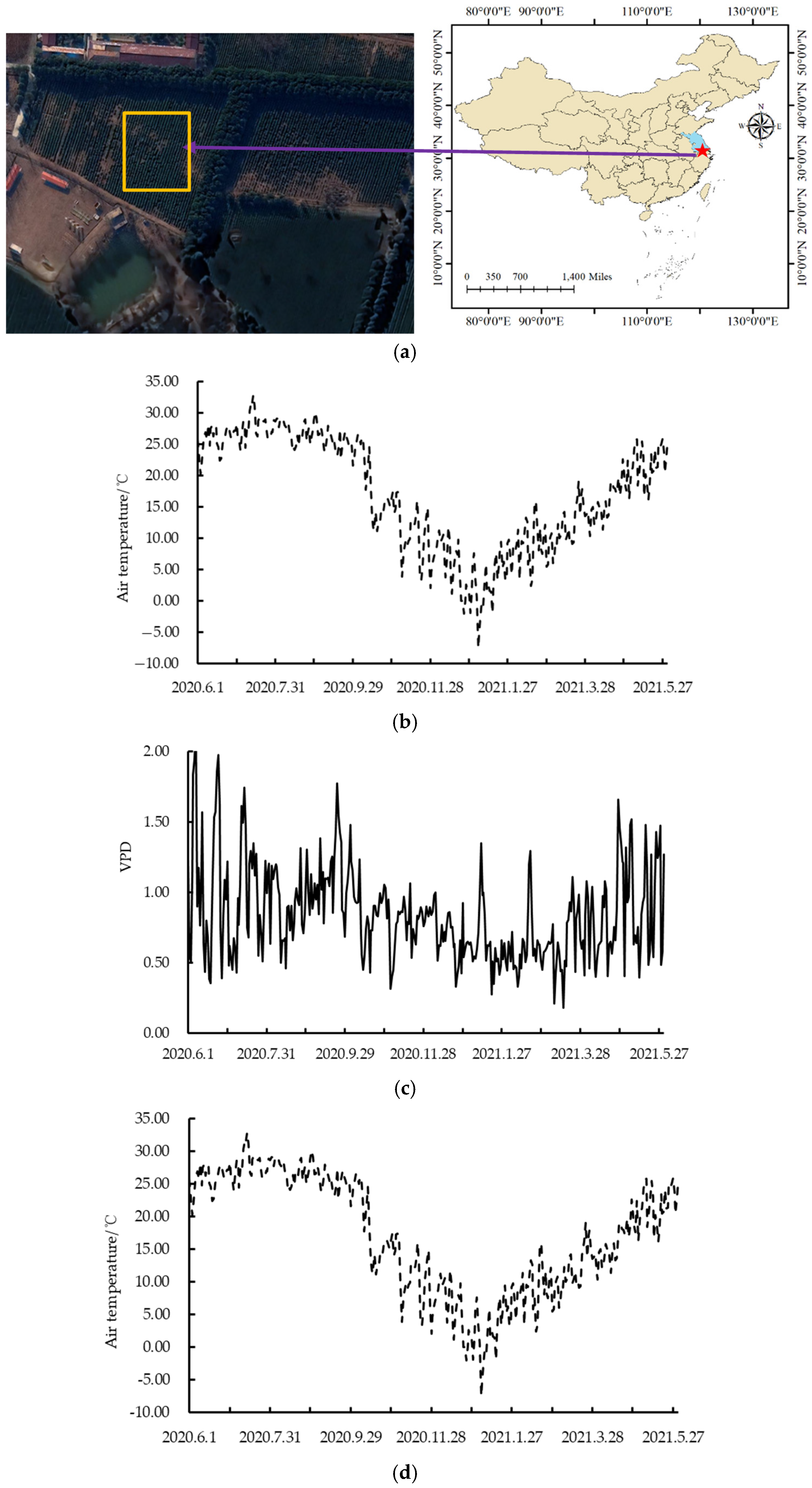
The experimental site, Maicun Tea Farm, is located in Danyang City, Jiangsu Province, China, within the low-slope hilly region that constitutes a major production area for high-quality tea in the middle and lower reaches of the Yangtze River (Figure 2a). The region has a mean annual temperature of 18.1 °C and an average annual precipitation of 1120.4 mm [3]. Despite generally favorable climatic conditions, rainfall is highly uneven in both temporal and spatial distribution, and periodic seasonal droughts frequently constrain tea yield and quality. At the time of the study, the tea plants were approximately six years old, and the plantation was fully established and in a stable production stage. Uniform management practices had been applied prior to the experiment, and no replanting or major structural changes occurred during the study period (from 1 June 2020 to 30 May 2021). The detailed micrometeorological data recorded during the field experiment are presented in Figure 2b–d. Micrometeorological data were continuously monitored during the experimental period using an automatic weather station installed adjacent to the experimental tea field. Air temperature and humidity at the height of 2.0 m were measured with HC2S3 (Campbell Scientific, Logan, UT, USA), respectively. All the sensors were calibrated before carrying out the experiment. CR3000 data loggers (Campbell Scientific, Logan, UT, USA) were used to collect the meteorological data, and the data sampling frequency of all the sensors was 0.5 Hz. The collection interval of all the sensors was 10 min.
The classification of soil texture is based on the World Reference Base (WRB) soil classification system [35]. The soil was collected from the experimental site at the depths of 0~10.0 cm, 10.0~20.0 cm, 20.0~30.0 cm, 30.0~40.0 cm, 40.0~50.0 cm and 50.0~60.0 cm. Bulk density and saturated volumetric water content (VWC) were measured by the oven dry method. A laser diffraction particle size analyzer (Mastersizer 3000, Malvern Panalytical, Malvern, WORC, UK) was used to measure the particle composition. The soil texture at the depth of 0~30.0 cm was sandy and under 30.0 cm was loam (Table 1). Time domain reflectometry (TDR) (CSC616, Campbell Scientific, Logan, UT, USA) was used to measure VWC and the measuring accuracy was ±1.0%. The soil water-holding characteristics were determined using the pressure plate apparatus method. Soil water retention curves were established by measuring volumetric water content at different matric potentials, allowing estimation of key parameters such as field capacity and wilting point [36].
The physical properties and the particle composition of the soil for the experiment are shown in Table 1. The maximum variation in field capacity remained consistent at 0.6%. Hence, it was reasonable to regard the soil within the 30.0–60.0 cm layer as homogeneous loam soil.

2.2. Determination of Tea Root Distribution and Wetted Ranges

Root excavation experiments were conducted in representative field plots under the stabilized drip irrigation treatments described in Table 2. Three representative tea plants were randomly selected from each treatment zone, and destructive sampling was performed after long-term drip irrigation operation to ensure that the observed root architecture reflected adaptation to the established soil moisture regime.
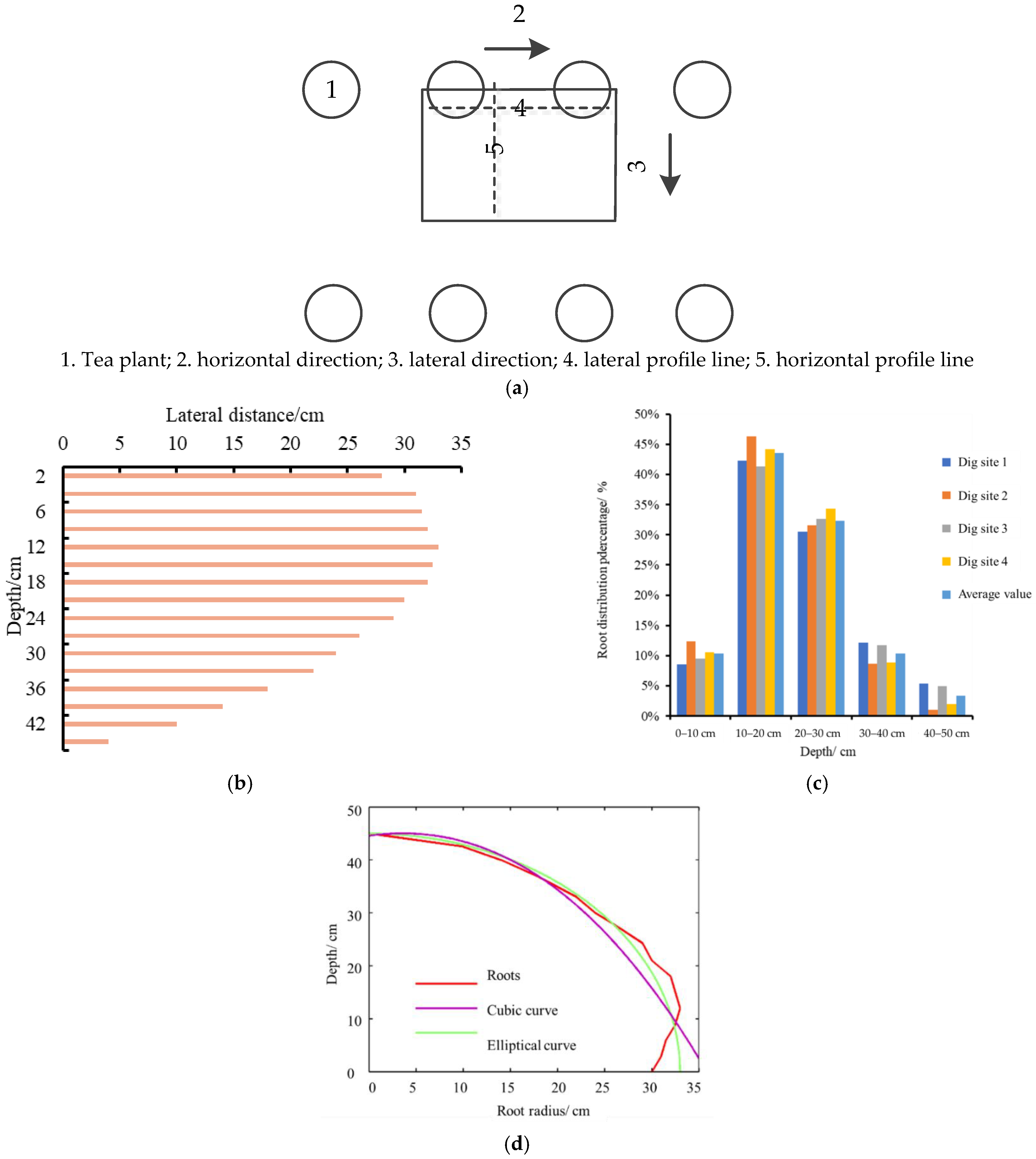
The experimental tea plantation adopted a planting pattern with plant spacing of 25.0–30.0 cm and row spacing of 160.0–180.0 cm. Soil profiles were excavated to a depth of 50 cm and divided into five layers at 10 cm intervals (0–50 cm) to quantify root distribution at different depths. Roots responsible for water and nutrient uptake were collected separately from each soil layer, and the proportion of roots in each layer was determined using the mass-based method.
To characterize root spatial distribution under drip irrigation, vertical distribution was quantified through layered sampling, whereas horizontal and lateral distributions were determined by measuring root extension distances from the taproot. The root distribution pattern was mathematically described using the cubic polynomial model (Equation (1)) and the elliptical model (Equation (2)) [29,37].
z = 0.00024 x 3 0.033 x 2 + 0.25 x + 45
x 2 a 2 + z 2 b 2 = 1
where a and b are the largest distances of tea roots in the lateral and vertical directions, respectively, cm; x is the lateral distance from the taproot, cm; and z is the vertical distance from the taproot, cm.
In addition, a series of drip irrigation treatments were designed with different emitter flow rates (1.0, 2.0, and 3.0 L·h−1), emitter spacings (40, 50, and 60 cm), and θ0 of 60%. A total of nine treatments (T1–T9) were established to further investigate the effects of irrigation parameters on soil water content distribution within the root zone. Each treatment combination of emitter spacing and discharge rate was maintained under field conditions until the wetting front reached the predetermined target depth (approximately 35–45 cm depending on treatment objectives). Soil water redistribution was monitored after irrigation cessation to capture post-irrigation equilibration processes. The root distribution data presented in Section 3.1 were obtained from destructive root sampling conducted within the same experimental field after long-term operation of the described drip irrigation system. The sampling was carried out under the stabilized irrigation configuration (i.e., using the same emitter layout and discharge conditions as defined in the experimental treatments). Therefore, the observed root architecture reflects plant adaptation to a sustained drip-irrigation-induced soil moisture regime rather than transient wetting events. This irrigation system design ensured that soil moisture dynamics, wetting front development, and root distribution characteristics were directly comparable across treatments, providing a consistent physical basis for linking irrigation parameters with root-zone development and soil water body (SWB) morphology. Soil water content (θs) is the volume of water relative to the field capacity value and is commonly expressed as a normalized ratio between the measured volumetric water content (VWC) and the soil volumetric water content at field capacity; it can be described as
θ s = θ V W C θ F C × 100
where θvwc is the measured volumetric water content (VWC), m3·m−3; and θFC is the volumetric water content at field capacity, m3·m−3.
To facilitate comparisons among soil layers with different field capacities, the measured volumetric water content (VWC) values were normalized relative to the field capacity of each soil layer. The normalized soil water content (θs) was expressed as the ratio between the measured VWC and the corresponding volumetric water content at field capacity. This normalization procedure minimized the influence of vertical heterogeneity in soil physical properties and enabled consistent evaluation of wetting-front migration and redistribution processes among treatments.

2.3. Experimental Design of Determining Drip Irrigation Parameters for Tea Fields

Soil texture significantly influences the morphological characteristics of the wetting front. In soils with relatively uniform texture, the water transport process can be considered isotropic, resulting in axisymmetric wetting patterns and water distribution [38,39]. Despite vertical variations in soil texture within the tea field, soils at the same depth exhibited homogeneous properties. Given the narrow spacing between tea plants and the dense horizontal distribution of tea roots, the overlap of wetting zones during drip irrigation is crucial for effectively moistening the root system. The degree of this overlap is influenced by various factors, including emitter spacing and flow rate. Therefore, the rational configuration of these parameters is essential for improving irrigation quality [40]. To determine optimal drip irrigation parameters, experiments were conducted to investigate the effects of different flow rates, emitter spacings, and θ0 on wetting front characteristics during the unidirectional intersection of two-point source drip irrigation. Laboratory tests were employed to analyze the wetting-front migration over time, the shape of the SWB, and post-irrigation water distribution, utilizing a quarter of the SWB for the analysis [41].
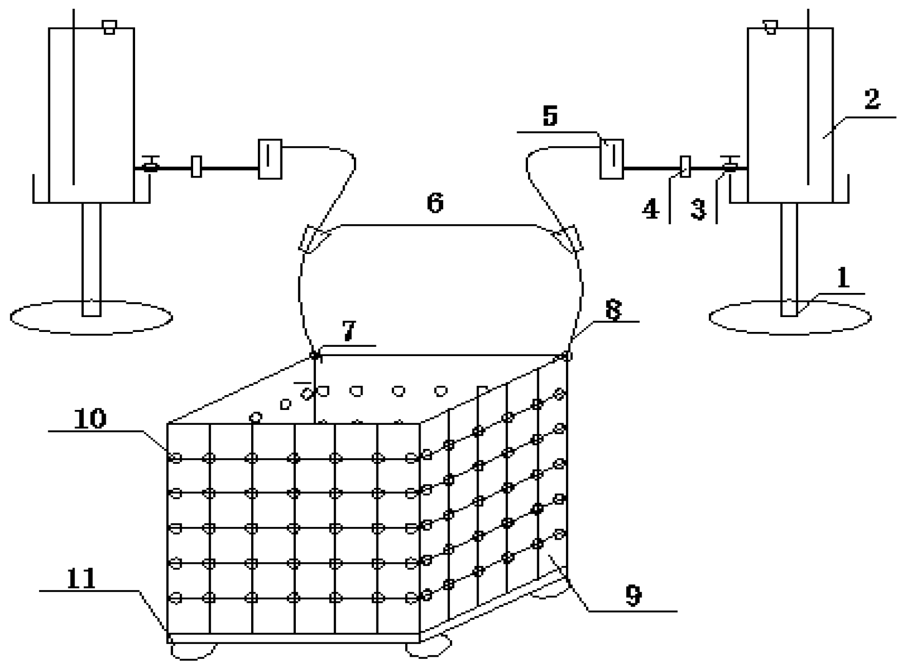
In the tea field, drip irrigation typically employs a flow rate of 1.0–3.0 L·h−1, with emitter spacing between 25.0 and 75.0 cm. Irrigation for approximately four hours is found to be most effective for achieving uniform water distribution and radial water movement [3]. An emitter spacing of 40.0–60.0 cm strikes an optimal balance. The experimental setup consists of two primary components: the water supply system and the soil tank (Figure 3). The water supply system comprises a base, a Mariotte bottle, a valve, hoses, a filter, a real-time flowmeter, a flow regulator, and an emitter. The Mariotte bottle serves dual functions: storing irrigation water and maintaining constant working pressure. The valve acts as a switch connected to the outlet of the Mariotte bottle, while hoses interconnect the various components to establish a continuous flow path. A real-time flowmeter (LSB-3WB) is used for continuous monitoring, offering a range of 4.0–40.0 mL·min−1. This allows for flow adjustments via the regulator, minimizing errors caused by flow deviations. To simulate actual drip irrigation processes, emitters were positioned on the soil surface.
The soil box, constructed from 8.00 mm thick acrylic, featured baffles on its base at 40.0 and 50.0 cm intervals to accommodate movable plates for varying emitter spacings. Through-holes (2.2 cm diameter) were placed at 10.0 cm intervals along the wall junctions and at a 3.0 cm offset on the side walls to facilitate sampling (Figure 3). To prevent deformation, the box was reinforced with bars at the base and sides, and steel wires at the upper, middle, and lower sections. A rubber plate with a wheel hub at the bottom allowed for easy repositioning.
A full factorial experiment was designed with three emitter discharges (1.0, 2.0, and 3.0 L·h−1) and three spacings (40.0, 50.0, and 60.0 cm), with two replicates per treatment (Table 2). Irrigation ceased upon reaching a vertical wetting depth of 35.0 cm, while the control group for redistribution analysis was set at 30.0 cm. Soil samples were collected from the tea field in 10.0 cm layers down to 60.0 cm after clearing surface debris. The soil was air-dried, sieved through a 2.0 mm mesh to remove debris, and stored in sealed bags. The initial gravimetric water content was measured via the oven-drying method. Subsequently, water was added to achieve 60.0% of field capacity, and the soil was thoroughly mixed and sealed for equilibration. The calculation formulas for soil and water mass are provided [42]:
m 0 = V s × γ
m 1 = 1 + θ m 0 × m 0
m 2 = 0.6 θ m θ m 0 × m 0
where γ is the bulk density of soil, g·cm−3; Vs is the volume of each layer of soil, d·m3; θ m is the field mass water capacity of each layer of soil, %; and m0, m1 and m2 are dry soil mass, air-dried soil mass and the added water mass, respectively, g.
Soil backfilling was conducted to maintain consistent depth and bulk density. The soil was packed in 5.0 cm layers to a total depth of 55.0 cm. To ensure adequate hydraulic contact between layers, the interface of each layer was roughened prior to adding the next. Upon completion, the exterior of the container was wrapped in plastic film to minimize sidewall evaporation, and the setup was allowed to equilibrate for 24 h before the drip irrigation experiment began.
Drip irrigation test procedures were conducted as follows: Firstly, the Mariotte bottle was filled with clean water and securely positioned at a fixed height on the stand. Valves were opened sequentially, and the flow rate was calibrated using a flow regulator, a stopwatch, a graduated cylinder, and the real-time flowmeter. Once the desired flow rate was achieved, the emitters were fixed above the intersecting surface of the container, positioned 1.0–3.0 cm above the soil surface and within 1.0 cm of the container wall. The experimental design simulated the one-directional intersection of a quarter of the wetting front. Ambient temperatures ranged from 26.0 to 33.0 °C; while natural evaporation from the soil surface occurred, its effect was considered negligible in the subsequent analysis.
The vertical infiltration depth directly beneath the emitter and the horizontal migration distance were defined as the vertical wetting front (Z) and horizontal wetting front (X), respectively. The intersecting profile beneath the emitter was defined as the O profile, whereas the non-intersecting side was defined as the P profile. Emitter discharge rate and cumulative irrigation volume were recorded throughout the experiment. Measurements of Z and X were taken at 1.0, 2.0, 5.0, 10.0, and 20.0 min during the initial infiltration stage, followed by measurements every 20 min until 2.0 h and every 30 min thereafter. Redistribution characteristics of the wetted body were further measured 24 h after irrigation ceased.
To evaluate wetting-body development and effective root-zone coverage, the wetting-front boundaries on both the O and P profiles were traced immediately after irrigation and again after 24 h of redistribution. Soil samples were collected from depths of 5.0, 15.0, 25.0, and 35.0 cm on both profiles immediately after irrigation and after the redistribution period. An additional soil sample was collected from the 45.0 cm depth after 24 h to assess deep percolation. Each soil sample (20.0–30.0 g) was weighed, and gravimetric water content was determined using the oven-drying method.
A randomized complete block design was adopted for field validation. Irrigation treatments were randomly assigned within the tea plantation to minimize spatial variability, with each treatment replicated twice. Soil samples were collected from multiple representative locations within each plot to improve spatial representativeness. Preliminary investigations confirmed that variations in soil texture and bulk density across the experimental area were minimal.

2.4. The Influence of Initial Soil Water Content on the Wetting Front

The optimal growth condition of tea plants was when the θ0 fell within the range of 70.0% to 90.0%. When this level dropped below 60.0%, there was a noticeable deceleration in growth. Typically, the θ0 at 60.0% was considered the threshold for initiating irrigation. However, depending on the growth stage of the tea plants, deficit irrigation may be employed to suppress growth, or alternatively, maintaining higher θ0 levels in the root zone may be prioritized to stimulate shoot and leaf growth. Additionally, θ0 also changed with the sequence of irrigation cycles. The lower limit of θ0 was typically set within the range of 50.0% to 70.0%. Different θ0 levels have a certain impact on the advancement of the wetting front. So, the single-factor experiment with five levels of θ0 with 50.0%, 55.0%, 60.0%, 65.0%, and 70.0% of field capacity was conducted to further analyze the characteristics of the wetting front for guiding the irrigation practice.
In order to more intuitively explain the water distribution in different wets, Chrischinson’s uniformity coefficient formula (Equation (7)) was used to calculate the uniformity coefficients of different surfaces [43].
C u = 1 i = 1 N θ i θ ¯ N × θ ¯ × 100 %
where Cu is the uniformity coefficient of SWB; θ i is the mass moisture content of the actual sampling point, %; N is the total number of samples; θ ¯ is the mean mass moisture content of the total sampling points. θ ¯ o , θ ¯ p , C u o , C u p is the mean and uniformity of soil water content on O and P profiles of SWB, respectively, %.

2.5. Validation Experiment of Optimal Control Strategy for Tea Field

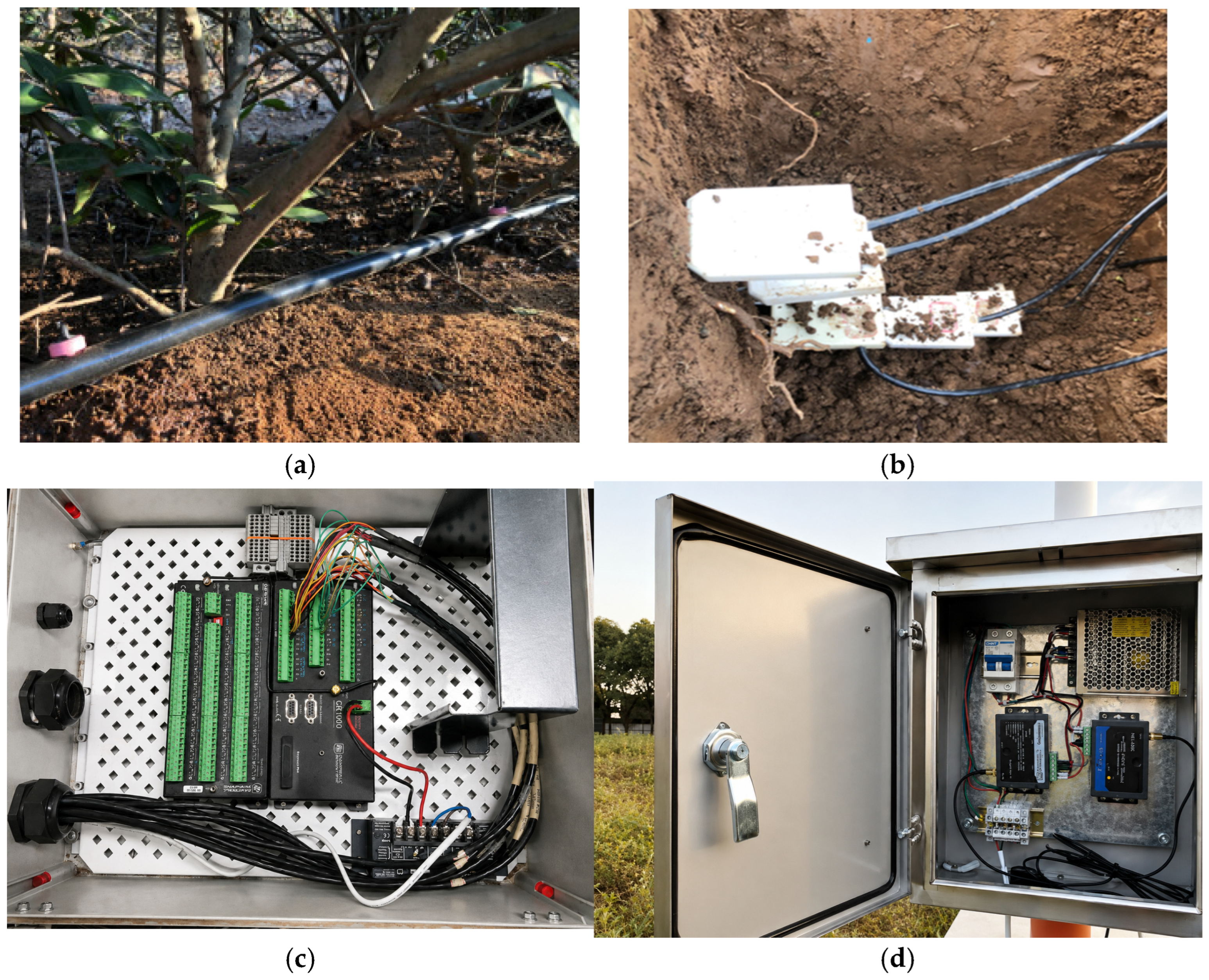
The traditional drip irrigation control process relies on water content measurements from a single soil layer, which often fails to accurately represent the water content throughout the entire root zone of tea plants [3]. However, soil content is a key parameter in drip irrigation management, influencing both the timing of irrigation and the dynamics of the wetting front [19]. In this experiment, six TDR sensors (CS616, Campbell scientific, Logan, UT, USA) were used to continuously measure θS in the root zone of the tea plants. These sensors were installed in the soil profile at a distance of 30.0 cm away from the tea plants, at 10.0 cm depth intervals, extending to a depth of 60.0 cm. A pre-drilled probe was used to insert the sensors. Data logging was carried out with a CR1000 data logger (Campbell Scientific, Logan, UT, USA), which recorded the θS readings on an hourly and daily basis. Due to the high correlation between adjacent soil layers, an equivalent model of soil water content was developed, where the moisture value from one layer was used to represent the moisture content of other highly correlated layers. To optimize sensor deployment, principal component analysis (PCA) was performed on the θS data at different depths. All the TDR sensors have been calibrated in the laboratory by using the oven dry method of measuring the VWC before installed in the experimental site. Two drip irrigation zones were set up in the field experiment, with each zone using 10 drip tapes, each tape being 36 m long and equipped with 90 emitters. All the emitters were 2.0 L·h−1 pressure-compensating emitters (Netafim, Tel Aviv, Israel) (Figure 4).
Irrigation zone one used the control strategy developed in this study, which controlled the initiation of drip irrigation based on a comprehensive evaluation of θS at 20.0 cm and 50.0 cm depths in the root zone, and calculated the drip irrigation time using the wetting front characteristic model. CS616 sensors were installed directly below the emitters. Irrigation zone two used a traditional control strategy, which directly took θS at a 20.0 cm depth as the input parameter to initiate drip irrigation and calculated the irrigation time with Equation (8) [44,45].
t 1 = 1000 V × η q × n × m × 60
where t1 is the total irrigation time of zone two, min; n is the number of drip taps; and m is the number of emitters on each drip tap.
The total irrigation time and irrigation amount of zone two can be described as [44]
t 1 = 1000 v × S θ v 1 θ v 0 × H q × n × m × 60
V = v × S θ v 1 θ v 0 × H η
where ν is the default wetting ratio, and it is set to 0.3; η is the water utilization coefficient, and it is set to 0.9. H is the target wetting depth, m, and it is set to 0.45; θv1 is the target soil water content for validation, and it is set to 0.351 (95% of field capacity). θv0 is the initial water content for validation, and it is set to 0.241 (65% of field capacity); S is the irrigation area, m2, and it is set to 660. The lower irrigation limit in irrigation zone one is set to 65% of field capacity, with a wetting depth of 45.0 cm; V is the total irrigation amount, m3.
At the start of irrigation, the starting date and time were recorded. During irrigation, the soil water content of the irrigation zone was sampled per minute. After stopping irrigation, the wetting width was measured using a tape measure. TDR sensor readings from various layers and the method of observation windows were used to determine the wetting depth comprehensively. The actual irrigation amount was collected from the water meter.
The water-saving rate was calculated by comparing the cumulative irrigation amount of the proposed control strategy (zone one) with that of the conventional irrigation strategy (zone two) over the same experimental period. The relative error in depth R e and water-saving rate η w were calculated by using Equations (11) and (12) [44].
R e = H 0 H H × 100 %
η w = V 1 V 0 V 1 × 100 %
where H0 is the actual wetting depth, m; V1 is the total irrigation amount under the conventional irrigation strategy, m3; and V0 is the total irrigation amount under the proposed wetting-front-based strategy, m3. Both irrigation zones were operated under identical climatic and field conditions to ensure comparability.

3. Results and Analysis

3.1. Tea Root Distribution Characteristics

Tea root distribution exhibited clear spatial regularity, characterized by a unimodal pattern with depth (Figure 5). Root density increased from 0 to 10 cm (8.6–12.4%) to a peak at 10–20 cm (42.3–46.3%), and then declined gradually, with 96.7% of the roots concentrated within 0–40 cm and the main absorption zone located at 10–30 cm (75.8%). Horizontally, the roots showed a symmetric distribution, with lateral extension first increasing and then decreasing, and the maximum distance occurring near 10 cm depth. The average vertical, horizontal, and lateral extensions were 43.3 cm, 33.0 cm, and 32.3 cm, respectively. Root interweaving among adjacent plants resulted in a relatively continuous interaction zone. Model fitting indicated that both cubic polynomial and elliptical functions performed well below 30 cm, whereas the elliptical model provided higher accuracy in shallow layers. Based on these characteristics, the effective wetted region under drip irrigation can be defined as an elliptical continuous zone within 0–45 cm depth and 0–35 cm lateral range, which represents the optimal target for irrigation management. Tea roots exhibited a well-defined distribution pattern in both vertical and horizontal directions, with a maximum rooting depth of approximately 45.0 cm (average 43.3 cm) and a maximum lateral extension of about 33.0 cm. Based on the measured data, both cubic polynomial equations and elliptical models were used to fit the root distribution, and the elliptical model was ultimately selected to define the effective wetted soil zone under drip irrigation, representing the main water distribution area.
Considering that absorption roots were distributed within the range of 0.0 to 45.0 cm vertically and 0.0 to 35.0 cm laterally, Table 2 indicates mean values of 43.3 cm vertically, and 33.0 cm and 32.3 cm horizontally and laterally, respectively. Therefore, the values of 33.0 cm and 45.0 cm can be utilized as follows:
x 2 33 2 + z 2 45 2 = 1
Below a depth of 30.0 cm, both methods adequately enveloped the root system. However, for the portion above 30.0 cm, the residual described by the elliptic equation was significantly smaller than that of the cubic polynomial. This indicated that the root system can be effectively enveloped by the elliptic equation (Figure 5). Consequently, the maximum wetted region of interest can be defined as the continuous wetted zone using the elliptic equation (Equation (13)) in the horizontal section.

3.2. The Characteristics of SWB Under Different Flow Rates and Emitter Spacings

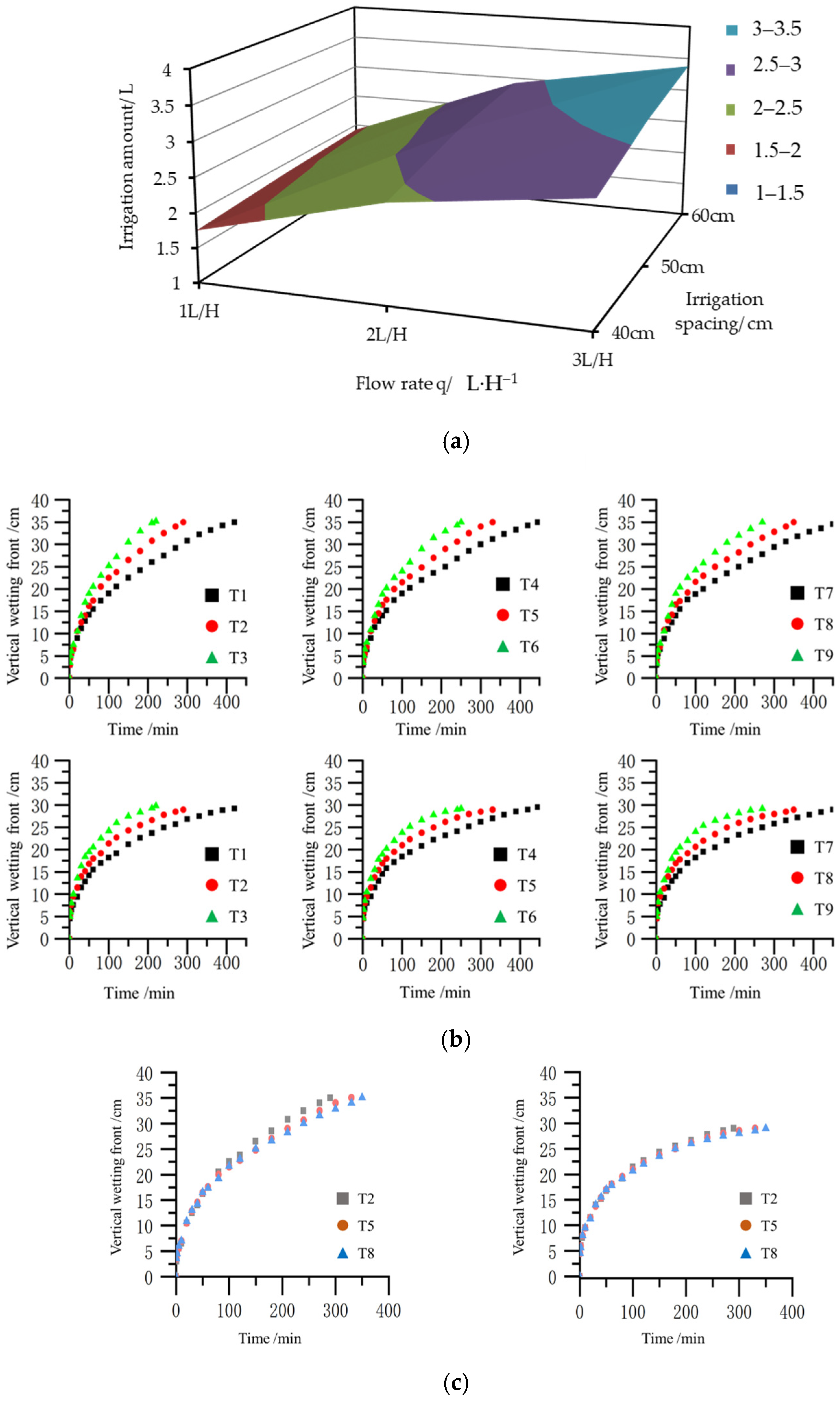
The total amount of irrigation water was influenced by the interaction between flow rate and spacing (Figure 6a), resulting in variations in irrigation time for the same termination depth. At flow rates of 1.0, 2.0, and 3.0 L·h−1, the differences in irrigation water volume across different spacings were 0.17 L, 0.50 L, and 0.63 L, respectively. Conversely, at spacings of 40.0, 50.0, and 60.0 cm, the differences in irrigation water volume across different flow rates were 1.0 L, 1.28 L, and 1.46 L, respectively.
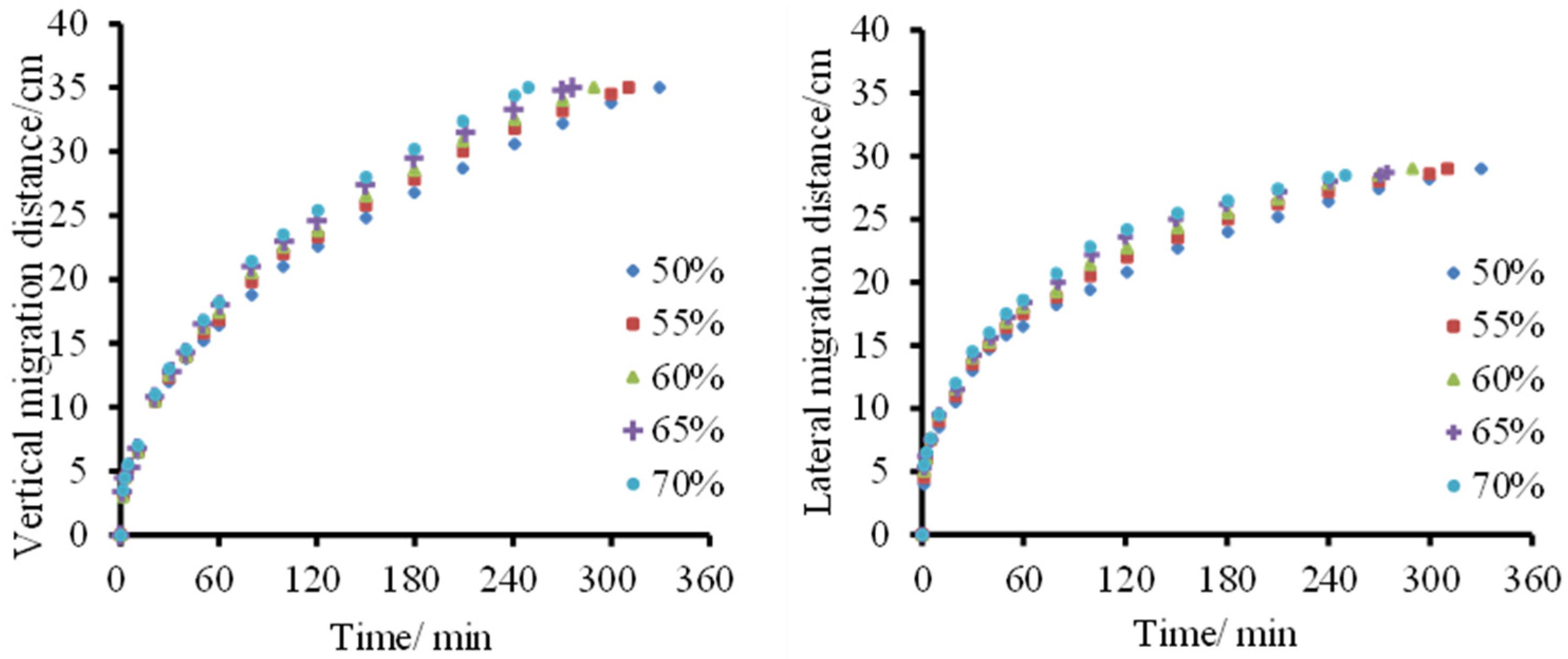
The dynamic changes in the wetting front showed that both X and Z values exhibited an increasing trend over irrigation time. However, as X and Z values gradually increased, the growth rates in all directions gradually slowed down. In the X direction, the growth rate began to plateau after the wetting front reached 28 cm, suggesting the existence of a maximum wetting radius for the drip irrigation system in the target tea field. Under the same spacing, changes in flow rate have a significant impact on the wetting front in all directions (Figure 6b). In the first 10 min of irrigation, the migration distances of the wetting front in the same direction are similar under different flow rates and do not show a consistent relationship with the flow rate. After 10 min of irrigation, different treatments begin to diverge. At the same time, the higher the flow rate, the larger the X and Z values, and the less time it takes to reach the same depth or width. This is because, over time, the total amount of irrigation water at the same moment becomes greater, and for high flow rate emitters, a saturated zone quickly forms below the emitter, driving the migration of X and Z. With different flow rates, the maximum difference in Z values at the same moment reaches 8.8 cm, and the maximum difference in X values reaches 6.8 cm.
Under a constant flow rate, spacing also notably impacted the wetting front (Figure 6c). Prior to convergence, X and Z values were similar across treatments. Post-convergence, the wetting fronts differentiated, with earlier convergence leading to larger X and Z values at the same moment. For instance, irrigation for treatments T2 and T5 ceased 60.0 and 20.0 min earlier, respectively, than for T8, indicating that convergence accelerated migration rates. However, the maximum differences in Z (2.8 cm) and X (1.1 cm) due to spacing were significantly smaller than those caused by flow rate variations.
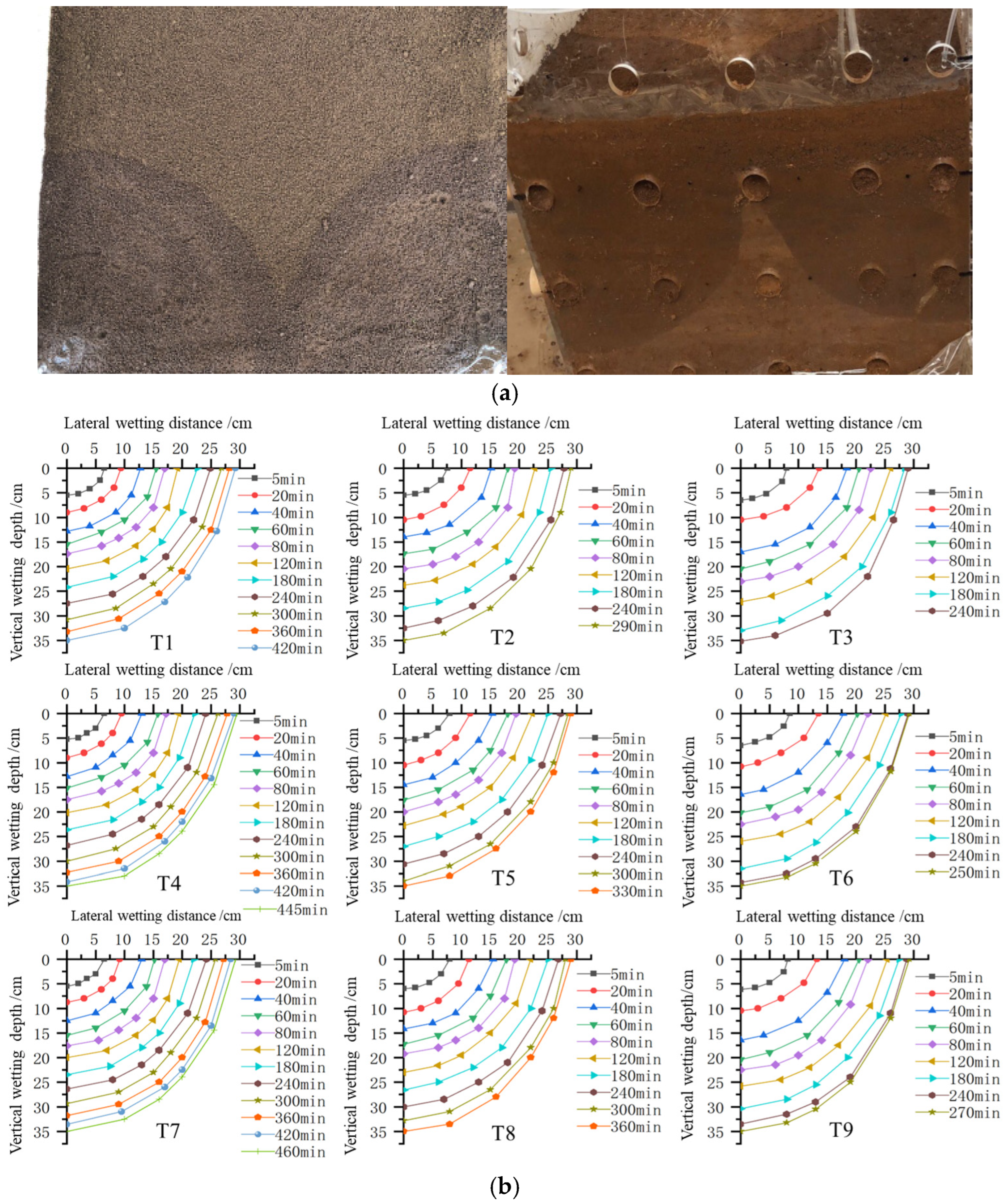
The wetted body exhibited an ellipsoidal shape (Figure 7a). The wetted range and the wetting front of the P profile under different treatments follow the same pattern, increasing over time but with a slowing growth rate. The wetted shape of the P profile appeared as a flat ellipse in the early stages of irrigation across different treatments (Figure 7b). Initially, the P profile appeared as a flat ellipse. As irrigation continued, the lateral infiltration rate decreased sharply while gravitational potential became dominant vertically. Consequently, the width-to-depth ratio approached 1, transforming the shape into a circle, and eventually fell below 1, resulting in a vertical ellipse.
Both flow rate and spacing have a noticeable impact on the wetted area of the P profile (Figure 7c). In the early stages of irrigation, the wetted area was relatively small, with insignificant differences among treatments. However, as the irrigation duration increased, distinct differences emerged. These differences were as follows: with constant spacing, treatments with higher flow rates resulted in a larger wetted area on the P profile for the same irrigation duration, i.e., T1 < T2 < T3, T4 < T5 < T6, T7 < T8 < T9. Conversely, with constant flow rates, the smaller the spacing, the shorter the time required for convergence at the same irrigation duration. After convergence, the wetted area on the P profile was larger, i.e., T1 > T4 > T7, T2 > T5 > T8, T3 > T6 > T9. At the end of irrigation, the combination of high flow rate and small spacing had the shortest duration, while the combination of low flow rate and large spacing had the longest duration. Although the differences in flow rate and spacing significantly impacted the irrigation duration and the wetted area at the same moment, the wetted area on the P profile for treatments T1 to T9 was similar at the end of irrigation. The shape of the wetted body was a vertical ellipse in all the treatments, indicating that flow rate and spacing mainly affected the rate of water movement. A similar wetted area can be achieved with low flow rates and large spacing by increasing the irrigation duration.
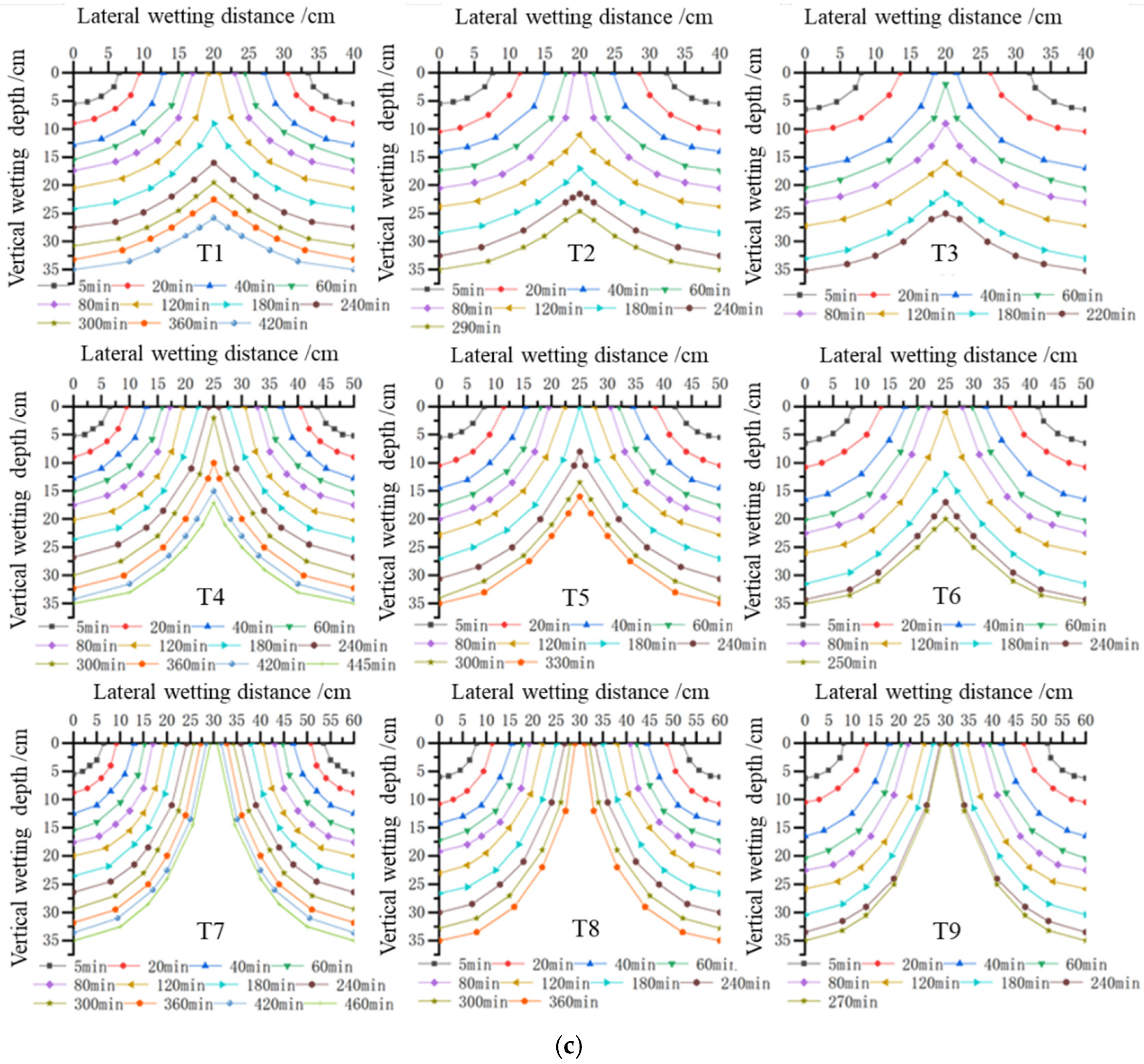
Both flow rate and spacing significantly influence convergence time. For a given spacing, the convergence times are T1 > T2 > T3 and T4 > T5 > T6. For a given flow rate, the convergence times are T1 > T4, T2 > T5, and T3 > T6. This demonstrates that higher flow rates and smaller spacings facilitate convergence, although the spacing should not exceed 60 cm. Prior to convergence, drip irrigation operated as point-source irrigation, with the O profile exhibiting characteristics similar to the P profile. After convergence, for a given flow rate, earlier convergence results in greater wetting depth at the same horizontal position. For instance, at 300 min of irrigation, the depth at the 10 cm horizontal position is 28 cm for T1 and 26 cm for T4. At 240 min of irrigation, the depth at the 12 cm horizontal position is 28 cm for T2 and 26.2 cm for T5.
At the end of irrigation, the shapes of the O profile were similar and the wetted areas were comparable for the same spacing but different flow rates. However, significant shape differences were observed with different spacings. This indicated that, for the direction of convergence, the shape of the O profile was primarily influenced by the degree of convergence. Smaller spacings result in larger convergence areas and flatter wetted body shapes. While different flow rates produced variations in the wetted range and shape of the O profile at the same moment, increasing the irrigation duration can achieve the same wetting effect with lower flow rates. Smaller emitter spacing increased the continuity of the wetted zone on the O profile.
When plant spacing is small and root systems are intertwined, a properly configured spacing can form a continuous wetted zone. Under different treatments, the P profile initially exhibited a flat elliptical shape in the early stages of irrigation. As the irrigation duration increased, it transitioned from a flat ellipse to a circle, and finally to a vertical ellipse (Figure 6c). Thus, the entire process of the P profile can be described as follows:
x 2 A 2 + z 2 B 2 = 1
where A is the lateral wetting length at different times, cm; B is the vertical wetting length at different times, cm.
During the filling process, A and B are variable values with t, which can be obtained from Equations (12) and (13); Equation (14) can be rewritten as
x 2 a × t b 2 + z 2 c × t d 2 = 1
To validate the effectiveness of the elliptical equation, we used treatment T2 as an example. We compared the P profile’s X and Z values and the actual wetted area at different times with the calculated values. The maximum errors for X and Z values were 0.9 cm and 1.4 cm, respectively, occurring at 40 min of irrigation. The maximum area difference was 20.6 cm2, occurring at 80 min of irrigation. The area difference initially increased and then decreased, while the ratio of area difference to total area showed a decreasing trend. After 80 min of irrigation, the deviation rate was less than 6.9% (Table 3). Therefore, the elliptical equation can be used to represent the wetted shape of the P profile.
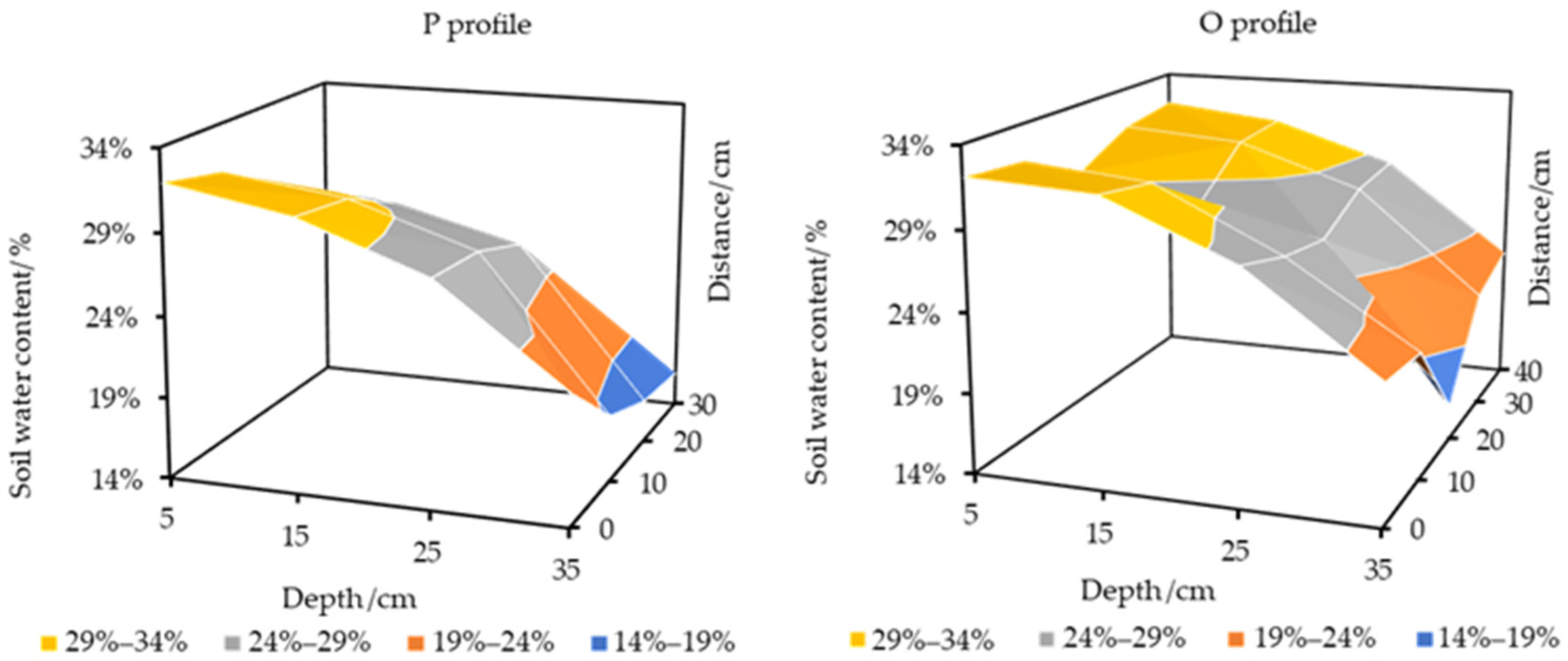
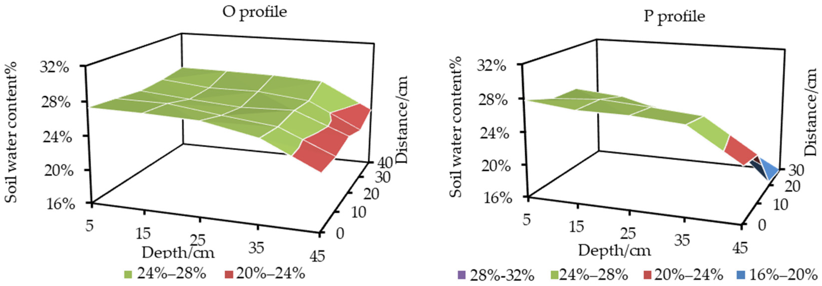
During the drip irrigation process, water gradually spreads from the outlet downward and outward. Variations in water requirements among different treatments to achieve the same depth result in inevitable differences in water distribution within the wetted zone (Figure 8). For the P profile, θs exhibited a decreasing trend with increasing depth and distance. Within a depth range of 15.0 cm and a radius of 10.0 cm, the θs exceeded 29%, indicating the formation of a water accumulation zone beneath the emitter. At the termination of irrigation, a distinct wetting front was discernible at a lateral distance of 29.0 cm from the emitter. Within the lateral span of 29.0 to 31.0 cm, the θs at depths of 5.0 cm and 15.0 cm were 21.8% and 18.1%, respectively, denoting an increase of approximately 5.5% in moisture content at the wetting-front boundary and a rise of approximately 2–3% in moisture content at distances of 3.0 to 5.0 cm from the wetting boundary. This underscored the necessity of a minimum 5% increase in moisture content to achieve a noticeable wetting front.
In the O profile, the convergence of wetting fronts occurred near a depth of 20.0 cm. Notably, the θs fluctuated significantly in soil layers at depths of 5.0 cm, 15.0 cm, and 35.0 cm, decreasing proportionally with increasing distance from the emitter. Conversely, θs in the soil layer at a depth of 25.0 cm remained relatively stable. Compared to the P profile, convergence elevated moisture content in the convergence zone and diminished the gradient of moisture variation between layers, resulting in a relatively uniform moisture distribution on this plane, particularly in soil layers at depths of 15.0 to 25.0 cm.
High flow rates and small spacing contributed to an increase in θ ¯ values, but C u values decreased with increasing flow rates and spacing. This is because larger flow rates result in higher water consumption at the end of irrigation, leading to a higher average moisture content within the wetted zone. However, the moisture is primarily concentrated near the emitter, increasing the moisture gradient within the wetted zone and reducing uniformity. For the same treatment, the moisture content and uniformity on the O profile were greater than those on the P plane. However, under different treatments, the uniformity on the P profile was relatively stable, while the O profile exhibited a larger fluctuation range. θ ¯ o , C u o , θ ¯ p and C u p values on the O profile ranged from 25.42% to 28.50%, 82.14% to 93.20%, 24.36% to 25.26%, and 80.12% to 82.39%, respectively (Table 4). In non-convergence directions, the fluctuation range of uniformity is small, whereas in the convergence direction, the degree of convergence (spacing) resulted in a larger fluctuation range of uniformity.

3.3. Soil Water Redistribution Characteristics

After drip irrigation ceased, the accumulated water around the emitter underwent soil water redistribution. As a result, changes occurred in the wetting front position, the geometry of the wetted body, and the spatial distribution of soil moisture. Across all the treatments, redistribution was essentially completed within 24 h after irrigation stopped.
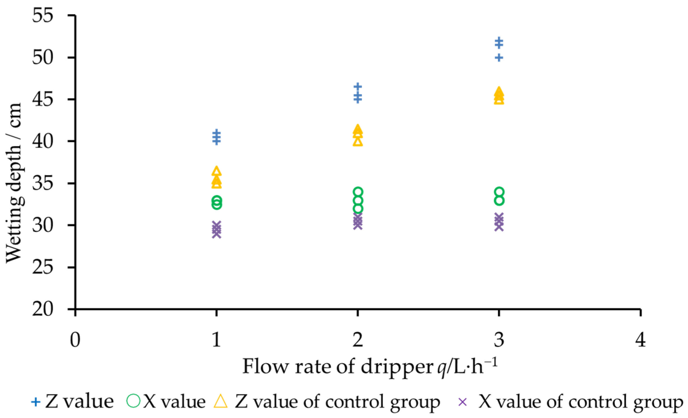
After 24 h of redistribution, the horizontal wetting front (X) for the different treatments ranged from 32.0 to 34.0 cm, corresponding to a redistribution distance of 3.0–5.0 cm (Figure 9). In comparison, the control group showed X values of 29.5–32.0 cm, with redistribution distances of 3.5–5.5 cm. Overall, the horizontal redistribution distances were similar among treatments and irrigation cutoff depths. In contrast, clear differences were observed in the vertical wetting front (Z). After redistribution, Z ranged from 40.0 to 52.0 cm with redistribution distances of 5.0–17.0 cm, whereas the control group ranged from 35.0 to 46.0 cm with redistribution distances of 5.0–16.0 cm. Higher emitter flow rates resulted in greater vertical redistribution distances. At the same flow rate, however, the redistribution distance of Z was comparable to the final migration distance. Specifically, for flow rates of 1.0, 2.0, and 3.0 L h−1, the redistribution distances of Z were 5.0–6.0 cm, 10.0–11.5 cm, and 15.0–17.0 cm, respectively; the control group showed similar ranges of 5.0–6.5 cm, 10.0–11.5 cm, and 15.0–16.0 cm. Using flow rate as the independent variable and the redistributed Z value as the dependent variable, a strong linear relationship was observed between Z and q at different irrigation cutoff depths, with R2 values exceeding 0.97.
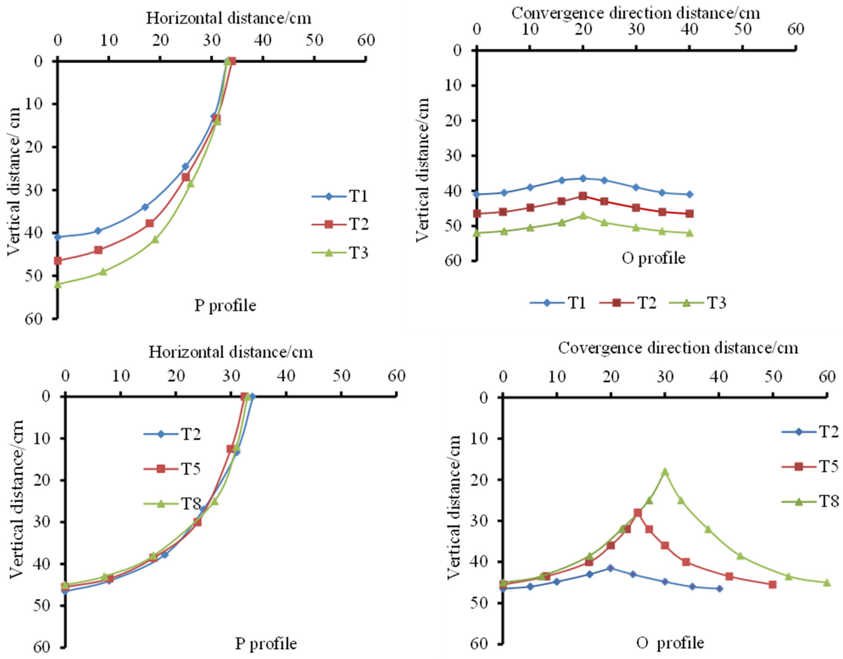
During the redistribution process, both the wetted areas on the O and P profiles underwent varying degrees of expansion, and convergence occurred when the spacing value was 60.0 cm. After irrigation stopped, moisture primarily moved in the Z direction, and the larger the flow rate, the larger the wetted areas on both the O and P profiles after redistribution. Although the flow rate affected the wetting depth, for the P profile, the wetted area remained approximately elliptical. The wetting front on the O profile was relatively flat, and the shape in the convergence direction was similar (Figure 10). After redistribution, higher emitter flow rates resulted in greater vertical redistribution depths.
Regardless of the same flow rate, the wetted area during the redistribution process increased with smaller spacing, leading to larger convergence and deeper wetting fronts at the convergence point. The fluctuation in the O profile decreased, and the wetting front became closer to a horizontal line. For the P profile, there were no significant differences under different spacings, and it can still be described using an elliptical equation. Therefore, spacing had a greater impact on the shape of the O profile, and smaller spacing was more conducive to forming a continuous drip irrigation belt (Figure 10).
Using treatment T2 as an example, the moisture distribution pattern after 24 h of redistribution is illustrated in Figure 10. Within the O profile, moisture distribution was relatively uniform, with θs ranging from 24% to 28% in the areas beyond 35.0 cm. Near the wetting front edge, soil water content remained above 20%. Within the P profile, as distance and depth increased, θs continued to decrease (Figure 11). However, in over 80% of the area within this plane, θs ranged from 24% to 28%, indicating a significantly improved uniformity of moisture distribution.
After 24 h of redistribution, the average moisture content and uniformity of the O and P profiles for each treatment are shown in Table 5. The average moisture content ranged from 22.92% to 27.03%, with the same spacing, increasing with higher flow rates. The fluctuation range was narrow, ranging from 23.03% to 24.68%, indicating small differences in moisture content among the P profile treatments. The uniformity ranged from 87.32% to 95.32% and from 81.42% to 85.48%. Compared to the moisture content at the end of irrigation, the average moisture content of each plane shows a decreasing trend, but the uniformity of moisture distribution is improved. This indicates that redistribution reduces water accumulation areas, decreases the gradient of moisture distribution, and effectively improves the quality of irrigation.

3.4. Determination of the Optimal Emitter Spacing and Flow Rate

When the spacing is 40.0 cm, the wetting front on the O profile of the wetted area approximated a horizontal straight line, indicating optimal continuity of the wetted zone. In contrast, spacings of 50.0 cm and 60.0 cm produced a continuous wavy pattern, and the continuity of the wetted region decreased as spacing increased, leading to a larger proportion of dry areas within the target wetting zone. Analysis of wetting uniformity further showed that closer spacing under identical flow conditions resulted in improved uniformity. Therefore, an emitter spacing of 40.0 cm was identified as optimal for the target tea field, with the possibility of further reducing spacing when a shallower wetting depth is required.
Since the migration rate of the X value slowed down after reaching 28.0 cm and the redistribution varies only between 3.0 and 5.5 cm across different treatments, while the Z value had a relatively higher rate, using the Z value as the criterion will improve control accuracy. In the target tea field, the maximum vertical root depth can reach up to 45.0 cm, but over 95% of the roots are distributed above 40.0 cm. Therefore, the wetting depth is typically set between 40.0 and 45.0 cm. To select the optimal flow rate, the vertical wetting depths of 45.0 cm and 40.0 cm are used, respectively.
When the target wetting depth is 40.0–45.0 cm, the required time for flow rates of 1 L·h−1, 2 L·h−1, and 3 L·h−1 is 427–593 min, 198–282 min, and 95–142 min, respectively. The total irrigation volumes are 7.12–9.88 L, 6.60–9.40 L, and 4.75–7.10 L, respectively, with lateral wetting distances of 33.7–37.2 cm, 30.4–33.5 cm, and 27.7–31.5 cm. At a flow rate of 1.0 L·h−1, the irrigation duration is the longest and the water usage is the highest, which increases irrigation energy consumption and is not conducive to water conservation. At a flow rate of 3.0 L·h−1, the irrigation time and water usage are the lowest, but it does not adequately wet the entire root zone. At a flow rate of 2.0 L·h−1, both the irrigation duration and water usage are moderate, and it can adequately wet the target area. Therefore, for the target tea field, a flow rate of 2.0 L·h−1 is optimal, making the T2 treatment suitable for the experimental tea field (Table 6).

3.5. Effect of Initial Soil Water Content on Wetting Front

Under different treatments, the smaller the θ0, the longer it took to reach the same depth (Table 7). The variations in the X and Z values over time under different initial θ0 are shown in Figure 12. Different θ0 values significantly impacted the migration process. Within the first 40 min before irrigation, the water migration distances for each treatment were comparable. However, after 40 min, differences between the treatments emerged. The higher the θ0 before irrigation, the faster the wetting front migrated in all directions, leading to a greater wetting distance for the same irrigation duration and a reduction in the total irrigation time and volume required. For the Z value, the differences between treatments became increasingly significant, whereas the differences in X initially increased and then decreased, with the maximum difference occurring around 120 min of irrigation. This is because the migration rate of X rapidly decreases after reaching 25.0 cm, and after 28.0 cm, the growth rate of the wetting front approximates a horizontal line. Therefore, using the Z value as the control parameter in drip irrigation projects can effectively reduce errors.
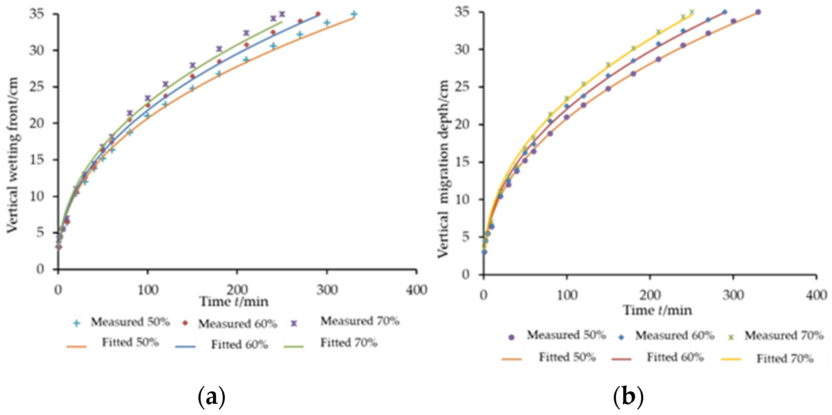
To quantitatively analyze the relationship between X, Z, and irrigation time (t) under different θ0, various treatments were fitted, with the results shown in Table 8. The values of X and Z with respect to t also followed a good power function relationship, with R2 values between 0.980 and 0.997. When θ0 varied between 50% and 70% of field capacity, the fitting parameters a, b, c, and d all changed. Among these, a (4.355–4.986) and c (2.871–3.055) fluctuated significantly, with a increasing as θ0 increased. In contrast, b (0.319–0.328) and d (0.427–0.440) showed smaller fluctuations, indicating that θ0 had a more significant impact on fitting parameters a and c.
Figure 13a shows the fitting curves and the trend of measured values for vertical migration distances when θ0 was 50%, 60%, and 70% of field capacity. In the early stages of irrigation, the measured values fitted well on the fitting curve, but as irrigation time increased, there was a greater deviation between the measured and fitted values. In the later stages of irrigation, the wetting-front migration rate was slower, and small distance deviations can cause larger time errors, reducing control accuracy when time is used as a control parameter. As θ0 increased, the wetting front rate also increased, resulting in larger values at the same time. According to the power function rule, when the exponent is constant, the larger the coefficient, the greater the dependent variable for the same independent variable. The fitting coefficients b and d are relatively stable, with mean values of 0.324 and 0.434, respectively (Table 8). Therefore, X and Z can be expressed as:
X = a × t 0.324
Z = c × t 0.434
X and Z were linearly fitted with t0.434 and t0.32, and R2 of both was above 0.982 (Table 9). Therefore, fitting parameters b and d with values of 0.324 and 0.434 could better describe the wetting front change process.
Figure 13b shows the variation trends of the measured values and fitting curves for different θ0 values when b and d were set to 0.324 and 0.434, respectively. In the early stages of irrigation, the curve values were greater than the measured values, but in the mid to late stages of irrigation, the measured values aligned well with the curve, with a high degree of accuracy. From a practical application perspective, the smaller the distance error in the mid to late stages of irrigation, the smaller the resulting time error, which greatly improved control accuracy when using time as the control parameter. Therefore, this curve is more suitable for practical drip irrigation engineering applications.
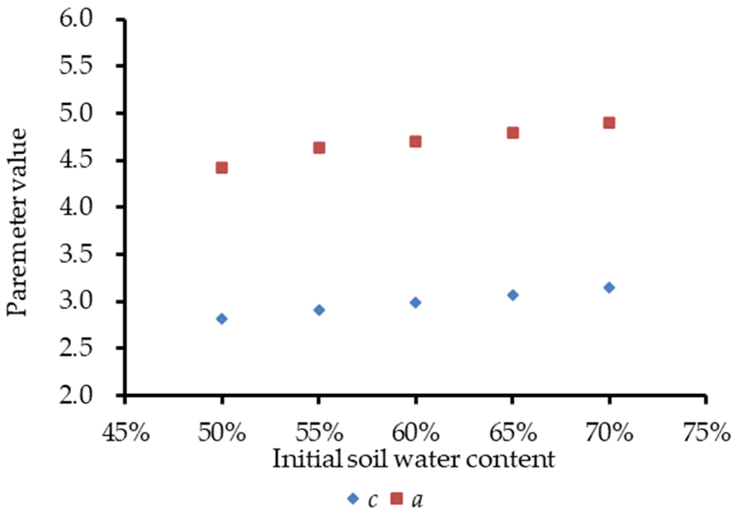
Both a and c tended to increase with the increase in θ0, where parameter a was 4.426, 4.642, 4.697, 4.789, and 4.901 respectively. The value of parameter c was 2.821, 2.915, 2.988, 3.067, and 3.152 (Figure 14).
The regression analysis was carried out on parameters a and c and the θ0. The results showed that a and θ0 had a good quadratic polynomial relationship (R2 is 0.969, p < 0.05), while c had a good linear relationship (R2 is 0.998, p < 0.05) with initial θ0, which can be expressed by the following equations, respectively:
a = 4.88 θ 0 2 + 8.0516 θ 0 + 1.6415
c = 1.6292 θ 0 + 2.0112
By putting the values of a and c into Equations (18) and (19), respectively, the functional relationship among X, Z, θ0 and t can be obtained as:
X = 4.88 θ 0 2 + 8.0516 θ 0 + 1.6415 × t 0.324
Z = 1.6292 θ 0 + 2.0112 × t 0.434
θ0 is different, and the profile change process of the wet body also follows the rule of changing from a horizontal ellipse to a vertical ellipse. Therefore, the P profile shape of the SWB during irrigation can be expressed as Equation (22):
x 2 4.88 θ 0 2 + 8.0516 θ 0 + 1.6415 × t 0.324 2 + z 2 1.6292 θ 0 + 2.0112 × t 0.434 2 = 1
After irrigation ended, water redistribution occurred, with Z increasing by 9.5 to 11.0 cm and X increasing by 3.6 to 5.2 cm. This indicated that changes in θ0 had little impact on the redistribution wetting distance, and flow rate remained the main factor affecting the redistribution range, consistent with previous research results. As θ0 increased, the total irrigation volume and duration decreased because less water was needed to reach saturation when the θ0 was higher. Consequently, the total amount of water required to wet the same area was also reduced, aligning with actual patterns. Therefore, at a flow rate of 2.0 L·h−1 and a spacing of 40.0 cm, the shape of the wetted area on the P profile after redistribution was completed under θ0 can be represented as
x 2 4.88 θ 0 2 + 8.0516 θ 0 + 1.6415 × t 0.324 + 4.4 2 + z 2 1.6292 θ 0 + 2.0112 × t 0.434 + 10.6 2 = 1

3.6. Determination of the Optimal Drip Irrigation Timing

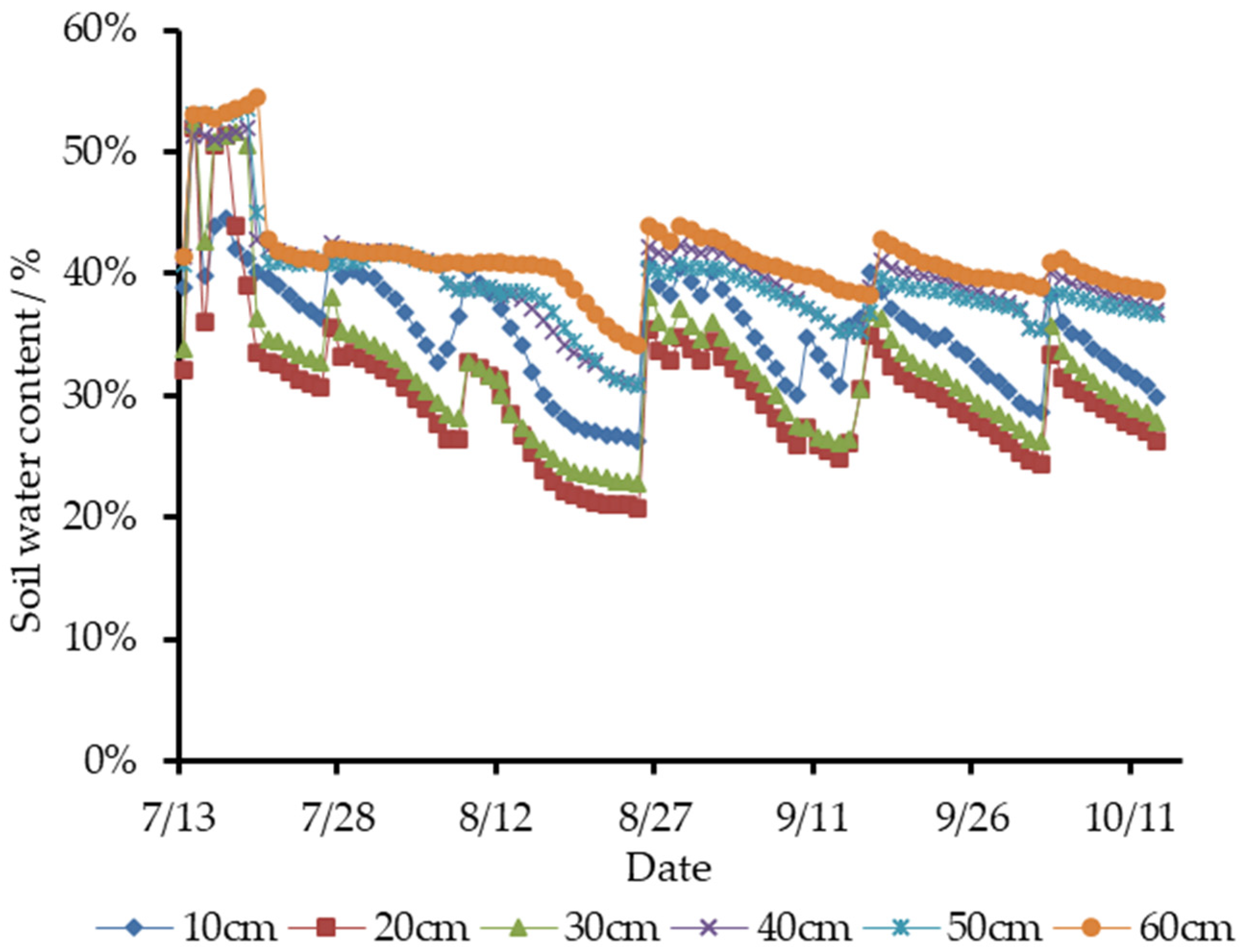
θs was the lowest at the 20.0 cm depth layer and highest at the 60.0 cm depth (Figure 15). θs across different layers showed minimal variation with an average difference of less than 2.7%. Significant fluctuations were observed at the 10.0 cm, 20.0 cm, and 30.0 cm depths, with coefficients of variation ranging from 0.141 to 0.160, all exhibiting a similar trend. In contrast, the θs at the 40.0 cm, 50.0 cm, and 60.0 cm depths remained relatively stable, with coefficients of variation between 0.089 and 0.097, also following a consistent trend. Based on these observations, the soil layers in the root zone can be classified into two distinct zones: a variable layer (0–30.0 cm) and a stable layer (30.0–60.0 cm) (Table 10).
The KMO and Bartlett’s confirmed the suitability of the dataset for factor analysis [46]. The KMO value was 0.813, falling within the 0.8–0.9 range, which indicates good sampling adequacy. Bartlett’s test was highly significant (p = 0.000 < 0.005), demonstrating strong correlations in soil water content among soil layers within the 0–60 cm profile. Linear correlation analysis further showed strong relationships between adjacent soil layers (Table 11). The correlation coefficients were 0.920 (10–20 cm), 0.972 (20–30 cm), 0.941 (30–40 cm), 0.965 (40–50 cm), and 0.935 (50–60 cm). In contrast, correlations declined as the distance between layers increased. The coefficients decreased to 0.865 (10–30 cm), 0.827 (10–40 cm), and 0.753 (10–50 cm), while the correlation between 40 cm and 60 cm remained relatively high at 0.898. These results indicate strong vertical coupling of soil moisture, particularly between adjacent layers, with progressively weaker relationships across larger depth intervals.
Typically, components with eigenvalues greater than 1 were selected. It can be observed that when using only one component, the cumulative variance contribution was only 89.7%, with more than 10.0% of information loss (Table 12). To better extract information from the original data and fully reflect the true soil moisture within the tea plant root layers, this study selected two principal components. The cumulative variance contribution reached 96.2%, with less than 4.0% of information loss.
The rotated component matrix results showed that the 10.0 cm, 20.0 cm, and 30.0 cm soil layers had relatively high loading proportions in component 2, with values of 0.902, 0.818, and 0.718, respectively (Table 13). On the other hand, the 40.0 cm, 50.0 cm, and 60.0 cm soil layers had relatively high loading proportions in component 1, with values of 0.781, 0.875, and 0.886, respectively. This indicated that the first principal component represents the soil water content of the variable layer, while the second principal component represents the soil water content of the stable layer.
Given the strong correlations between adjacent soil layers, sensors can be strategically installed at 20.0 cm (variable layer) and 50.0 cm (stable layer). Using θs at 10.0, 30.0, 40.0, and 60.0 cm as dependent variables and the measurements at 20.0 cm and 50.0 cm as independent variables, simple linear regression was applied to develop an equivalent estimation model. The resulting models achieved coefficients of determination (R2) greater than 0.846, indicating good agreement between predicted and observed values. (Table 14).
In order to better calculate the soil water content of the root layer, it can be considered that the dynamic change in soil water content of adjacent soil was continuous, which can be obtained according to the mean value theorem of integrals:
θ v = Δ h H s S W 1 + S W 2 + S W 3 + + S W n 1 + 1 2 S W 1 + S W n
where θ v is the soil water content in the root layer; Δ h is the distance between adjacent measuring points, cm; H s is the depth of the soil, cm; S W i is the soil volumetric water content of different depth measuring points; n is the soil depth of the measuring points, and they are 10, 20⋯, and 60.0 cm, respectively.
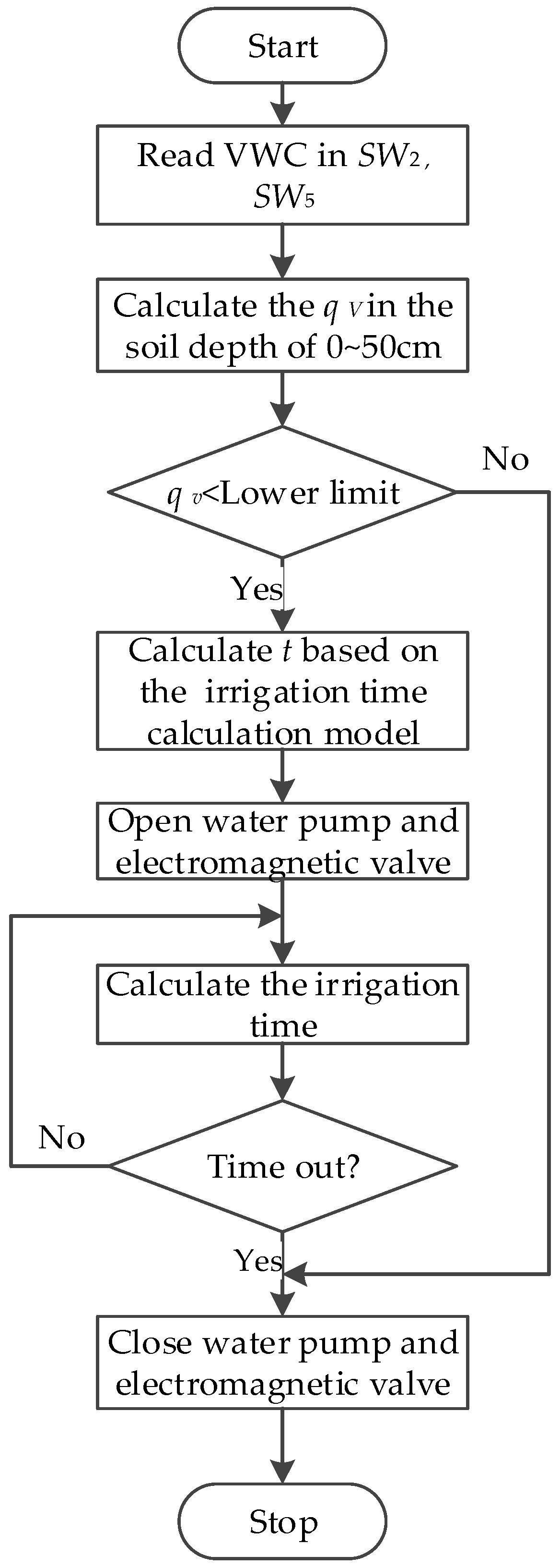
The root depth in the experimental site is 45.0 cm, so the H s is 50.0 cm and the Δ h is 10.0 cm; the θv can be obtained according to the soil water content equivalent model.
θ v = 10 50 3 2 S W 1 + S W 2 + S W 3 + S W 4 + 1 2 S W 5
So the relationship model among θ v , SW2 and SW5 can be described as
θ v = 0.655 S W 2 + 0.2794 S W 5 + 0.0446
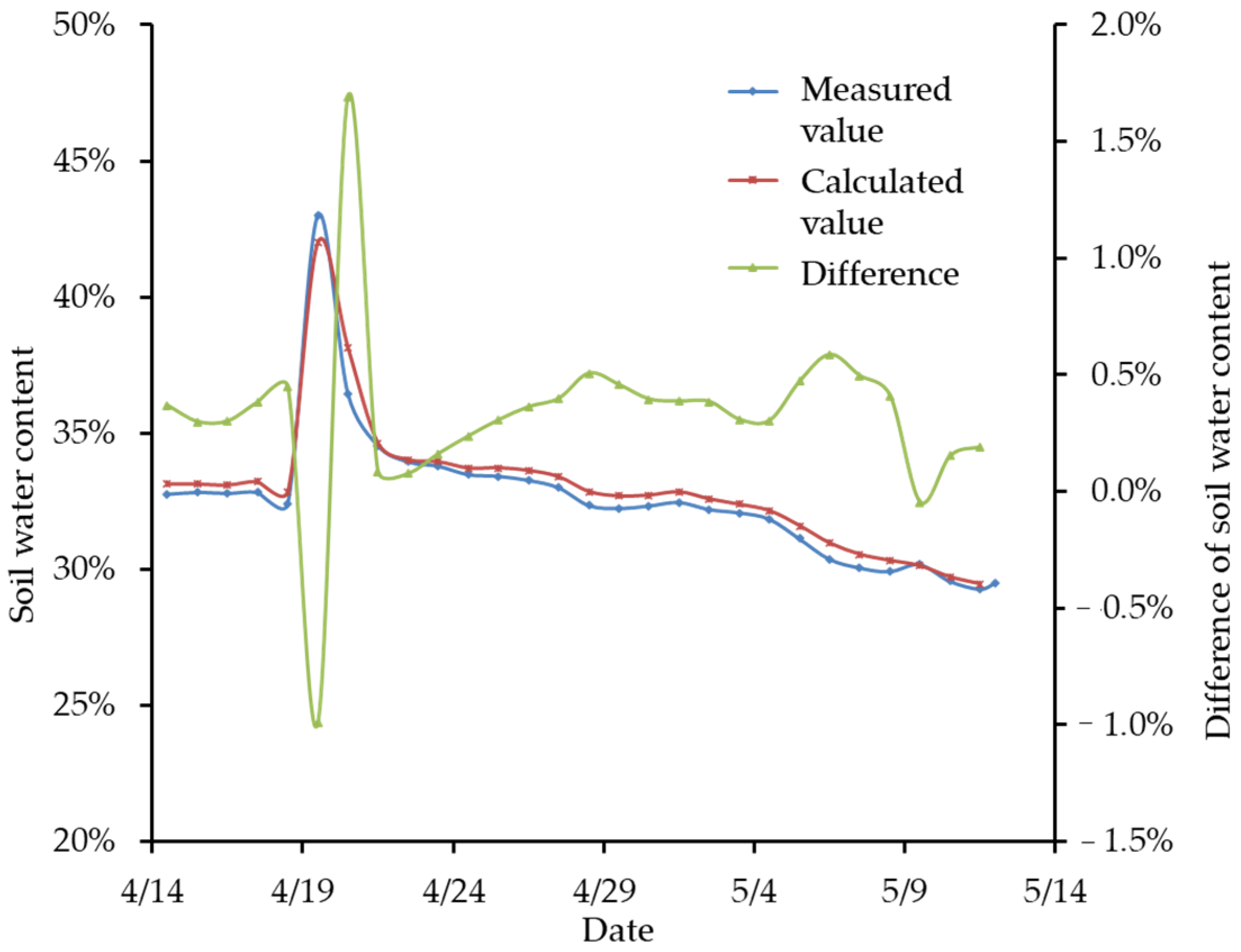
The validation test results indicated that the deviation fluctuates around 0. According to meteorological data, there was a heavy rainfall event from 19–20 April 2021. During the rainfall phase and the subsequent moisture redistribution phase, there were significant differences between the measured and calculated values of soil water content, with the peak difference reaching 1.7%. The model’s calculated values were smaller during the rainfall process but larger during the redistribution process. In non-precipitation periods, the model’s calculation accuracy was higher, with deviations fluctuating within ±0.7%, meeting the accuracy requirements for practical application (Figure 16).
In addition, since the migration distance of the wetting front in different directions has a good functional relationship with t and θ0, it is assumed that the target wetting width and depth are A0 and B0, respectively. A0 and B0 can be expressed as:
A 0 = 4.88 θ 0 2 + 8.0516 θ 0 + 1.6415 × t 0.324 + 4.4
B 0 = 1.6292 θ 0 + 2.0112 × t 0.434 + 10.6
Equations (27) and (28) can be deformed as:
t 0.324 = A 0 4.4 4.88 θ 0 2 + 8.0516 θ 0 + 1.6415
t 0.434 = B 0 10.6 1.6292 θ 0 + 2.0112
So t can be described as:
t = A 0 4.4 4.88 θ 0 2 + 8.0516 θ 0 + 1.6415 1 0.324
t = B 0 10.6 1.6292 θ 0 + 2.0112 1 0.434
Therefore, in practical applications, once the θ0 before irrigation and the target wetting range (width or depth) are given, the irrigation time can be determined based on the wetting-front migration pattern. For the wetting front, in the later stages of irrigation, as the wetted area expands and the soil’s infiltration capacity decreases, both Z and X rates decrease. However, the migration rate of Z is much larger than that of X. Although obtaining X is simpler in actual engineering, using X as a control reference to calculate irrigation time is more complex. Moreover, after X reached 25.0 cm, the rate became very slow, and small distance errors can cause significant time fluctuations, leading to reduced system control accuracy. Therefore, in practical applications, using a vertical migration model to determine irrigation time is more reliable (Figure 17).

3.7. Performance Experiment Results of Drip Irrigation Control Strategy

When irrigation zone one was started, the θs at a depth of 20.0 cm was 0.202 and the actual relative water content in the root zone was 65%, which matched the expectation (Table 15). When irrigation zone two was started, the θs at a depth of 20.0 cm was 0.240 and the actual relative water content in the root zone was 73%. It exceeded the expected value and resulted in early irrigation.
At the end of irrigation, the total applied water volumes for zone one and zone two were 8.30 m3 and 10.07 m3, respectively. The wetting depth and horizontal wetting distance for zone one were 35.5 cm and 27.8 cm, respectively, while for zone two, they were 41.0 cm and 29.5 cm, which were 5.5 cm and 1.7 cm greater than zone one, respectively. After redistribution, the wetting depth increased to 47.5 cm in zone one and 52.5 cm in zone two, exceeding the target wetting depth by 2.5 cm and 7.5 cm, respectively. At the moment irrigation ceased, the θs at 20 cm depth in zone two reached 0.396, exceeding field capacity and indicating substantial internal soil water accumulation. After 24 h of redistribution, the relative water content within the upper 50 cm soil layer reached 98%, a condition unfavorable for tea plant growth.
Compared with traditional drip irrigation control systems, the tea field drip irrigation control system in this study had higher precision in controlling the wetting depth. The measured wetting depth error was within 5.6%, which was 11.1% less than the error of the traditional method, effectively avoiding deep percolation issues. In terms of water-saving benefits, this control technology saved 17.6% more water compared to traditional drip irrigation control technology.

4. Discussion

The present study demonstrated that SWB development in tea plantation drip irrigation follows a clear time-dependent evolution process controlled by the interaction between capillary and gravitational forces. During the initial irrigation stage, matric potential gradients dominated water movement, resulting in rapid lateral expansion of the wetting front and formation of a horizontally elongated wetted body. As irrigation continued, gravitational potential gradually became dominant, accelerating downward infiltration and transforming the SWB from a flat ellipse into a near-circular shape and eventually into a vertically elongated ellipse. Similar infiltration dynamics have been widely reported in drip irrigation studies based on Richards equation simulations and field experiments in orchard and row-crop systems, where the wetting front transitions from capillary-controlled lateral flow to gravity-driven vertical percolation under prolonged irrigation conditions [23,36,40]. However, compared with previous studies, the current work provides a more explicit geometric characterization of this transition process by simultaneously analyzing both the O-profile (convergence direction) and P-profile (vertical section), thereby improving the mechanistic interpretation of wetted body evolution in shallow-rooted tea plantations.
Emitter spacing was identified as the primary structural factor controlling SWB continuity and moisture distribution uniformity. Reducing emitter spacing significantly improved wetting front convergence in the O profile and enhanced the formation of a continuous wetted belt [47]. The 40 cm spacing treatment produced the highest wetting continuity and minimized dry zones within the effective tea root distribution region. This agrees with recent state-of-the-art studies on surface and subsurface drip irrigation, which emphasize that overlapping adjacent wetted bulbs is essential for improving root-zone water uniformity and reducing localized water stress. Nevertheless, compared with orchard crops such as citrus and grapevine, the optimal spacing identified in this study was relatively smaller. The low-slope hilly tea plantation environment may weaken preferential flow effects compared with coarse-textured orchard soils, thereby increasing the importance of emitter convergence for moisture uniformity [48].
Flow rate primarily regulated wetting-front migration velocity and irrigation duration. Higher discharge rates accelerated both horizontal and vertical infiltration because rapid local saturation beneath the emitter increased hydraulic conductivity in the near-field saturated zone. Similar conclusions have been reported in previous hydraulic studies of drip irrigation systems, where emitter discharge strongly influences infiltration rate and wetting front advancement but exerts less influence on the final equilibrium wetted geometry [49]. In the present study, although higher flow rates produced larger wetted areas during irrigation, the final wetted body shape among treatments converged toward a similar vertically elliptical structure after sufficient irrigation duration. This indicates that emitter layout and convergence degree had greater influence on SWB geometry than discharge rate itself. Low flow rates required excessively long irrigation times and higher total water consumption, whereas excessively high flow rates reduced lateral wetting continuity and increased localized water accumulation near emitters [50].
The redistribution process after irrigation cessation further demonstrated the dominant role of gravitational drainage in SWB evolution. Redistribution mainly increased wetting depth rather than lateral expansion, confirming that vertical hydraulic gradients controlled post-irrigation water movement. Similar redistribution patterns have been reported in orchard drip irrigation systems and vadose-zone infiltration studies. However, the redistribution magnitude observed in this study was relatively moderate, likely because the experimental tea soil possessed relatively fine texture and moderate antecedent moisture content, which limited excessive preferential downward flow. Redistribution also improved moisture uniformity by reducing water accumulation near the emitter and decreasing spatial moisture gradients. The improvement in uniformity after redistribution indicates that irrigation evaluation based solely on conditions immediately after irrigation termination may underestimate the final effectiveness of water distribution within the root zone.
The proposed strategy improved irrigation efficiency while maintaining reliable soil moisture regulation within the target root zone. Compared with the current state-of-the-art precision irrigation systems based on remote sensing, machine learning, or evapotranspiration estimation, the present approach has stronger physical interpretability because irrigation decisions are directly linked to subsurface wetting dynamics and root-zone water distribution. However, unlike UAV-assisted or IoT-driven intelligent irrigation systems, the proposed framework still has limited adaptability to rapidly changing environmental conditions and lacks automatic integration with real-time meteorological variability and crop physiological responses.
Despite these strengths, several limitations should be acknowledged. First, the experiments were conducted under relatively homogeneous soil conditions and controlled field settings. Natural tea plantations often exhibit considerable heterogeneity in soil texture, bulk density, slope, and preferential flow pathways, which may influence wetting-front behavior and reduce model transferability. Second, although the simplified elliptical model provides strong engineering applicability, it cannot fully capture the complexity of three-dimensional unsaturated flow processes resolved by advanced Richards equation numerical simulations or stochastic hydraulic conductivity models. Third, the study mainly focused on soil hydraulic behavior and did not explicitly integrate plant physiological indicators such as stomatal conductance, canopy temperature, sap flow, or photosynthetic response. Modern precision agriculture increasingly combines soil sensing with crop physiological monitoring and UAV-based multispectral analysis to achieve adaptive irrigation scheduling. Finally, the experiments were conducted under a specific tea plantation environment, and further validation across different soil textures, climatic conditions, slopes, and tea cultivation systems is still required.

5. Conclusions

This study investigated the morphological evolution of the SWB under different drip irrigation flow rates and emitter spacings, with the objective of improving irrigation management for tea plantations. By systematically analyzing irrigation volume, wetting front dynamics (X and Z), SWB geometry, and soil water content distribution, suitable irrigation parameters were identified for the experimental field.
For a given irrigation termination depth, both irrigation volume and wetted area increased with higher flow rates and wider emitter spacing. However, the combination of a higher flow rate and closer emitter spacing resulted in the shortest irrigation duration. Wetting-front migration was strongly governed by flow rate, whose influence was more pronounced than that of emitter spacing. In contrast, spacing primarily controlled the degree of wetting-front convergence and the spatial uniformity of soil water content. Reduced spacing enhanced overlap between adjacent wetted zones, producing a flatter SWB and improving irrigation uniformity. These results suggest that increasing flow rate is an effective strategy for reducing irrigation time, whereas decreasing emitter spacing is more beneficial for improving wetted zone continuity and irrigation quality.
The SWB profile on the P section evolved from a horizontally elongated ellipse to a vertically oriented ellipse, which could be well described using an elliptical function. At the end of irrigation, soil water content decreased with increasing distance from the emitter, forming a clearly defined wetting front. Subsequent redistribution further improved irrigation quality by expanding the wetted area and reducing moisture gradients. The increases in X and Z ranged from 3.0 to 5.5 cm and 5.0–17.0 cm, respectively, and showed strong dependence on flow rate. Continuous monitoring of soil water content at depths of 20 and 50 cm enabled the development of a soil water content equivalence model with an error below 1.7%. When combined with a predefined lower irrigation threshold, this model accurately predicted irrigation initiation. Compared with conventional drip irrigation control, the proposed approach achieved a water saving of 17.6%, demonstrating its potential for improving water-use efficiency in tea cultivation.

Author Contributions

Y.L. and W.W. conceived and designed the experiments. Y.L. and W.W. performed the experiments and analyzed the data. Y.L. and W.W. wrote the manuscript. Y.L., P.L., and Y.H. gave some significant comments to improve the quality and language of the manuscript. All authors have read and agreed to the published version of the manuscript.

Funding

This research was funded by the Project Funded by the Basic Public Welfare Special Project of Shaoxing City (2025A13001) and Priority Academic Program Development of Jiangsu Higher Education Institutions (PAPD 2023-87).

Data Availability Statement

The original contributions presented in this study are included in the article. Further enquiries can be directed to the corresponding author.

Acknowledgments

We would like to express our gratitude to all reviewers for their patience and help.

Conflicts of Interest

The authors declare no conflicts of interest.

References

  1. Xu, Q.; Yang, Y.; Hu, K.; Chen, J.; Djomo, S.N.; Yang, X.; Knudsen, M.T. Economic, Environmental, and Emergy Analysis of China’s Green Tea Production. Sustain. Prod. Consum. 2021, 28, 269–280. [Google Scholar] [CrossRef] [Scilit]
  2. Zhen, H.; Qiao, Y.; Ju, X.; Hashemi, F.; Knudsen, M.T. Organic Conversion Tea Farms Can Have Comparable Economic Benefits and Less Environmental Impacts than Conventional Ones—A Case Study in China. Sci. Total Environ. 2023, 877, 162698. [Google Scholar] [CrossRef] [Scilit]
  3. Lu, Y.Z.; Liu, P.F.; Montazar, A.; Paw U, K.T.; Hu, Y.G. Soil Water Infiltration Model for Sprinkler Irrigation Control Strategy: A Case for Tea Plantation in Yangtze River Region. Agriculture 2019, 9, 206. [Google Scholar] [CrossRef] [Scilit]
  4. Sun, M.; Jia, X.; Yang, D.; Lu, B.; Han, F.; Shi, F. Life Cycle Environmental Impact Assessment of Green Tea Production in China. J. Clean. Prod. 2024, 434, 140377. [Google Scholar] [CrossRef] [Scilit]
  5. Lin, S.K.; Lin, J.; Liu, Q.L.; Ai, Y.F.; Ke, Y.Q.; Chen, C.; Zhang, Z.Y.; He, H. Time-Course of Photosynthesis and Non-Structural Carbon Compounds in the Leaves of Tea Plants (Camellia sinensis L.) in Response to Deficit Irrigation. Agric. Water Manag. 2014, 144, 98–106. [Google Scholar] [CrossRef] [Scilit]
  6. Luo, Y.P. China Tea Cultivation; China Agricultural Press: Beijing, China, 2015. [Google Scholar]
  7. Safaei Chaeikar, S.; Marzvan, S.; Jahangirzadeh Khiavi, S.; Rahimi, M. Changes in Growth, Biochemical, and Chemical Characteristics and Alteration of the Antioxidant Defense System in the Leaves of Tea Clones (Camellia sinensis L.) under Drought Stress. Sci. Hortic. 2020, 265, 109257. [Google Scholar] [CrossRef] [Scilit]
  8. Santos, E.L.R.; Rezende, F.P.; Moron, S.E. Stress-Related Physiological and Histological Responses of Tambaqui (Colossoma macropomum) to Transportation in Water with Tea Tree and Clove Essential Oil Anesthetics. Aquaculture 2020, 523, 735164. [Google Scholar] [CrossRef] [Scilit]
  9. Yan, H.; Yu, J.; Zhang, C.; Wang, G.; Huang, S.; Ma, J. Comparison of Two Canopy Resistance Models to Estimate Evapotranspiration for Tea and Wheat in Southeast China. Agric. Water Manag. 2021, 245, 106581. [Google Scholar] [CrossRef] [Scilit]
  10. Yan, H.; Deng, S.; Zhang, C.; Wang, G.; Zhao, S.; Li, M.; Liang, S.; Jiang, J.; Zhou, Y. Determination of Energy Partition of a Cucumber Grown Venlo-Type Greenhouse in Southeast China. Agric. Water Manag. 2023, 276, 108047. [Google Scholar] [CrossRef] [Scilit]
  11. Zhang, C.; Zhang, W.; Yan, H.; Ni, Y.; Akhlaq, M.; Zhou, J.; Xue, R. Effect of Micro–Spray on Plant Growth and Chlorophyll Fluorescence Parameter of Tomato under High Temperature Condition in a Greenhouse. Sci. Hortic. 2022, 306, 111441. [Google Scholar] [CrossRef] [Scilit]
  12. Issaka, Z.; Li, H.; Jiang, Y.; Tang, P.; Chao, C. Comparison of rotation and water distribution uniformity using dispersion devices for impact and rotary sprinklers. Irrig. Drain. 2019, 68, 881–892. [Google Scholar] [CrossRef] [Scilit]
  13. Li, H.; Issaka, Z.; Jiang, Y.; Tang, P.; Chen, C. Overview of Emerging Technologies in Sprinkler Irrigation to Optimize Crop Production. Int. J. Agric. Biol. Eng. 2019, 12, 1–9. [Google Scholar] [CrossRef] [Scilit]
  14. Wang, J.; Yang, T.; Wei, T.; Chen, R.; Yuan, S. Experimental Determination of Local Head Loss of Non-Coaxial Emitters in Thin-Wall Lay-Flat Polyethylene Pipes. Biosyst. Eng. 2020, 190, 71–86. [Google Scholar] [CrossRef] [Scilit]
  15. Zheng, Z.; He, Y.; He, Y.; Zhan, J.; Shi, C.; Xu, Y.; Wang, X.; Wang, J.; Zhang, C. Micro-Nano Bubble Water Subsurface Drip Irrigation Affects Strawberry Yield and Quality by Modulation of Microbial Communities. Agric. Water Manag. 2025, 307, 109228. [Google Scholar] [CrossRef] [Scilit]
  16. Zhang, C.; Li, J.; Yan, H.; Akhlaq, M.; Xue, R.; Disasa, K.N.; Lakhiar, I.A.; Ren, J.; Hameed, M.U. Exploring Uniformity of Temperature Distribution Within and Above the Canopy Using a Distributed Fibre-Optic Temperature Sensing Under a Natural and Forced Ventilation Greenhouse. N. Z. J. Crop Hortic. Sci. 2026, 54, e70005. [Google Scholar] [CrossRef] [Scilit]
  17. Zhou, Y.; Bao, R.; Yan, H.; Zhang, C.; Zheng, H.; Wu, J.; Zhang, J.; Wang, G.; Tian, D.; Xue, R.; et al. Optimization of Shallow Buried Drip Irrigation and Nitrogen Management for Spring Maize in the Sandy Land of Northwest China. Field Crops Res. 2025, 333, 110056. [Google Scholar] [CrossRef] [Scilit]
  18. Xue, R.; Zhang, C.; Yan, H.; Disasa, K.N.; Lakhiar, I.A.; Akhlaq, M.; Hameed, M.U.; Li, J.; Ren, J.; Deng, S.; et al. Determination of the Optimal Frequency and Duration of Micro-Spray Patterns for High-Temperature Environment Tomatoes Based on the Fuzzy Borda Model. Agric. Water Manag. 2025, 307, 109240. [Google Scholar] [CrossRef] [Scilit]
  19. Choi, Y.B.; Shin, J.H. Development of a Transpiration Model for Precise Irrigation Control in Tomato Cultivation. Sci. Hortic. 2020, 267, 109358. [Google Scholar] [CrossRef] [Scilit]
  20. Li, J.; Jin, H.; Wang, C.; Wang, H. A New Method of Estimating Soil Water Diffusivity Based on Variation in the Wetting Front Position and on the Principle of Stationary Action. J. Hydrol. 2022, 612, 128290. [Google Scholar] [CrossRef] [Scilit]
  21. Wang, H.; Wang, H.; Liang, X.; Wang, J.; Qiu, X.; Wang, C.; Li, G. Infiltration Simulation and System Design of Biogas Slurry Drip Irrigation Using HYDRUS Model. Comput. Electron. Agric. 2024, 218, 108682. [Google Scholar] [CrossRef] [Scilit]
  22. Zamani, S.; Ostad-Ali-Askari, K.; Nafchi, R.F.; Provenzano, G. Assessing a Semi-Empirical Model Performance to Predict the Wetting Patterns in Subsurface Drip Irrigation. Clean. Water 2024, 1, 100020. [Google Scholar] [CrossRef] [Scilit]
  23. Naglič, B.; Kechavarzi, C.; Coulon, F.; Pintar, M. Numerical Investigation of the Influence of Texture, Surface Drip Emitter Discharge Rate and Initial Soil Moisture Condition on Wetting Pattern Size. Irrig. Sci. 2014, 32, 421–436. [Google Scholar] [CrossRef] [Scilit]
  24. Dabral, P.P.; Pandey, P.K.; Pandey, A.; Singh, K.P.; Singh, M.S. Modelling of Wetting Pattern under Trickle Source in Sandy Soil of Nirjuli, Arunachal Pradesh (India). Irrig. Sci. 2012, 30, 287–292. [Google Scholar] [CrossRef] [Scilit]
  25. Chu, S.-T. Green-Ampt Analysis of Wetting Patterns for Surface Emitters. J. Irrig. Drain. Eng. 1994, 120, 414–421. [Google Scholar] [CrossRef] [Scilit]
  26. Schwartzman, M.; Zur, B. Emitter Spacing and Geometry of Wetted Soil Volume. J. Irrig. Drain. Eng. 1986, 112, 242–253. [Google Scholar] [CrossRef] [Scilit]
  27. Al-Ogaidi, A.A.M.; Wayayok, A.; Rowshon, M.K.; Abdullah, A.F. Wetting Patterns Estimation under Drip Irrigation Systems Using an Enhanced Empirical Model. Agric. Water Manag. 2016, 176, 203–213. [Google Scholar] [CrossRef] [Scilit]
  28. Zhang, S.; Han, X.; Cruse, R.M.; Zhang, X.; Hu, W.; Yan, Y.; Guo, M. Morphological Characteristics and Influencing Factors of Permanent Gully and Its Contribution to Regional Soil Loss Based on a Field Investigation of 393 Km2 in Mollisols Region of Northeast China. CATENA 2022, 217, 106467. [Google Scholar] [CrossRef] [Scilit]
  29. Ben-Asher, J.; Charach, C.; Zemel, A. Infiltration and Water Extraction from Trickle Irrigation Source: The Effective Hemisphere Model. Soil Sci. Soc. Am. J. 1986, 50, 882–887. [Google Scholar] [CrossRef] [Scilit]
  30. Hachum, A.Y.; Willardson, L.S.; Alfaro, J.F. Water Movement in Soil from Trickle Source. J. Irrig. Drain. Div. 1976, 102, 179–192. [Google Scholar] [CrossRef] [Scilit]
  31. Kanda, E.K.; Senzanje, A.; Mabhaudhi, T. Modelling Soil Water Distribution under Moistube Irrigation for Cowpea (VIGNA unguiculata (L.) Walp.) Cro. Irrig. Drain. 2020, 69, 1116–1132. [Google Scholar] [CrossRef] [Scilit]
  32. Ye, J.; Wang, C.; Chen, X.; Kurexi, W.; Huang, M.; Duan, Z.; Xu, R.; Li, Y.; Zhang, Z. Experimental and Numerical Investigations on Soil–Water Dynamics in Moistube Irrigation under Dynamically Regulated Working Pressure Heads: Scenario Simulations under Maize Cultivation. J. Hydrol. 2024, 634, 131083. [Google Scholar] [CrossRef] [Scilit]
  33. Chen, R.; Li, H.; Wang, J.; Guo, X.; Xiang, Y. Evaluating Soil Water Movement and Soil Water Content Uniformity under Sprinkler Irrigation with Different Soil Texture and Irrigation Uniformity Using Numerical Simulation. J. Hydrol. 2023, 626, 130356. [Google Scholar] [CrossRef] [Scilit]
  34. Winter, T.C.; Harvey, J.W.; Franke, O.L.; Alley, W.M. Ground Water and Surface Water: A Single Resource; Circular: Washington, DC, USA, 1998. [Google Scholar]
  35. FAO. World Reference Base for Soil Resources 2014: International Soil Classification System for Naming Soils and Creating Legends for Soil Maps; FAO: Rome, Italy, 2014; ISBN 978-92-5-108369-7. [Google Scholar]
  36. Richards, L.A. Porous plate apparatus for measuring moisture retention and transmission by soil. Soil Sci. 1948, 66, 105. [Google Scholar] [CrossRef] [Scilit]
  37. Vigo, Á.D.; Zubelzu, S.; Juana, L. Infiltration Models and Soil Characterisation for Hemispherical and Disc Sources Based on Green-Ampt Assumptions. J. Hydrol. 2021, 595, 125966. [Google Scholar] [CrossRef] [Scilit]
  38. Verdi, A.; Naseri, M. Effects of Tire Wear Particles on the Water Retention of Soils with Different Textures in the Full Moisture Range. J. Contam. Hydrol. 2024, 264, 104345. [Google Scholar] [CrossRef] [Scilit]
  39. Zhu, Z.; Li, J.; Zhu, D.; Gao, Z. The Impact of Maize Canopy on Splash Erosion Risk on Soils with Different Textures under Sprinkler Irrigation. CATENA 2024, 234, 107608. [Google Scholar] [CrossRef] [Scilit]
  40. Samoy-Pascual, K.; Lampayan, R.M.; Remocal, A.T.; Orge, R.F.; Tokida, T.; Mizoguchi, M. Optimizing the Lateral Dripline Spacing of Drip-Irrigated Aerobic Rice to Increase Water Productivity and Profitability under the Water-Limited Condition. Field Crops Res. 2022, 287, 108669. [Google Scholar] [CrossRef] [Scilit]
  41. Shiri, J.; Karimi, B.; Karimi, N.; Kazemi, M.H.; Karimi, S. Simulating Wetting Front Dimensions of Drip Irrigation Systems: Multi Criteria Assessment of Soft Computing Models. J. Hydrol. 2020, 585, 124792. [Google Scholar] [CrossRef] [Scilit]
  42. Kaiser, M.; Kleber, M.; Berhe, A.A. How Air-Drying and Rewetting Modify Soil Organic Matter Characteristics: An Assessment to Improve Data Interpretation and Inference. Soil Biol. Biochem. 2015, 80, 324–340. [Google Scholar] [CrossRef] [Scilit]
  43. Burt, C.; Styles, S.W. Drip and Microirrigation for Trees, Vines, and Row Crops (with Special Sections on Buried Drip); Irrigation Training and Research Center, Department of Agricultural Engineering, California Polytechnic State University: San Luis Obispo, CA, USA, 1994; ISBN 978-0-9643634-0-3. [Google Scholar]
  44. Burt, C.M.; Styles, S.W. Drip and Micro Irrigation Design and Management for Trees, Vines, and Field Crops-Practice plus Theory, 3rd ed.; Irrigation Training and Research Center, Ed.; Irrigation Training and Research Center: San Luis Obispo, CA, USA, 2007; ISBN 978-0-9643634-4-1. [Google Scholar]
  45. Tang, P.; Li, H.; Issaka, Z.; Chen, C. Effect of Manifold Layout and Fertilizer Solution Concentration on Fertilization and Flushing Times and Uniformity of Drip Irrigation Systems. Agric. Water Manag. 2018, 200, 71–79. [Google Scholar] [CrossRef] [Scilit]
  46. Bartlett, M.S. The effect of standardization on a χ2 approximation in factor analysis. Biometrika 1951, 38, 337–344. [Google Scholar] [CrossRef] [Scilit]
  47. Zhang, Q.; Wang, Q.; Wang, Z. Decreasing Soil Water Repellency during Infiltration: Linking Time-Dependent Contact Angle to a Physically Meaningful Scaling Parameter. J. Hydrol. 2026, 670, 135225. [Google Scholar] [CrossRef] [Scilit]
  48. Vishwakarma, D.K.; Kumar, R.; Abed, S.A.; Al-Ansari, N.; Kumar, A.; Kushwaha, N.L.; Yadav, D.; Kumawat, A.; Kuriqi, A.; Alataway, A.; et al. Modeling of Soil Moisture Movement and Wetting Behavior under Point-Source Trickle Irrigation. Sci. Rep. 2023, 13, 14981. [Google Scholar] [CrossRef] [Scilit]
  49. Jha, S.K.; Gao, Y.; Liu, H.; Huang, Z.; Wang, G.; Liang, Y.; Duan, A. Root Development and Water Uptake in Winter Wheat under Different Irrigation Methods and Scheduling for North China. Agric. Water Manag. 2017, 182, 139–150. [Google Scholar] [CrossRef] [Scilit]
  50. Ma, X.; Sanguinet, K.A.; Jacoby, P.W. Direct Root-Zone Irrigation Outperforms Surface Drip Irrigation for Grape Yield and Crop Water Use Efficiency While Restricting Root Growth. Agric. Water Manag. 2020, 231, 105993. [Google Scholar] [CrossRef] [Scilit]
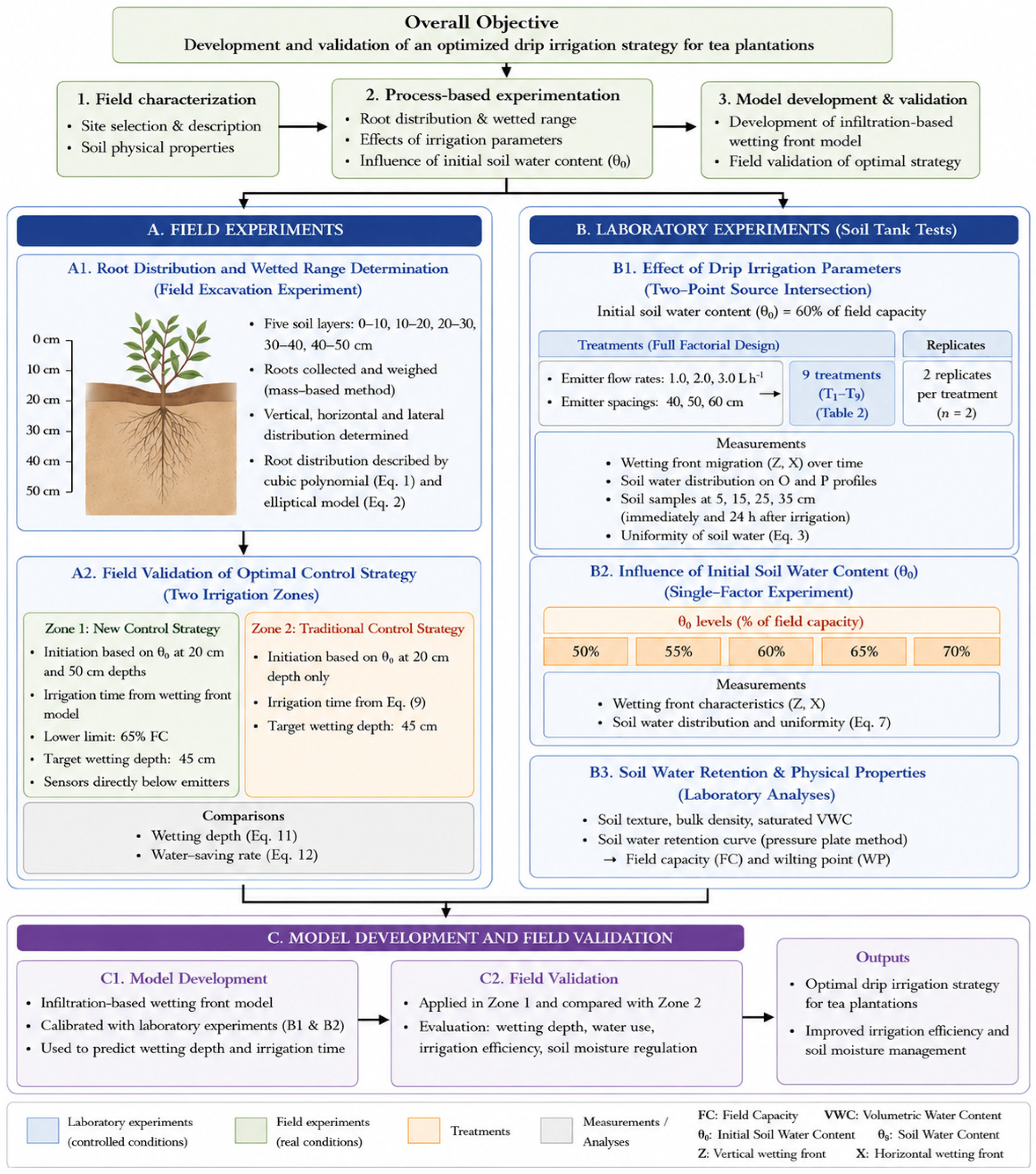
Figure 1. Flowchart of this research.
Agronomy 16 01089 g001
Figure 2. Location and background micrometeorological data of the experimental tea field from 1 June 2020 to 30 May 2021: (a) Location of the experimental tea field. (b) Relative humidity dynamic change with time. (c) Vapor pressure deficit dynamic change with time. (d) Air temperature dynamic change with time.
Agronomy 16 01089 g002
Figure 3. Drip irrigation testing system. 1. A base; 2. Markov bottle; 3. valve; 4. filter; 5. real-time flowmeter; 6. flow regulator; 7. irrigator; 8. hose; 9. soil box plate; 10. soil sampling holes; 11. rubber plate with a wheel hub.
Agronomy 16 01089 g003
Figure 4. Validation experiment of the new control strategy: (a) Drip irrigation tape layout. (b) CS616 sensors layout. (c) Data acquisition node. (d) Smart gateway.
Agronomy 16 01089 g004
Figure 5. Tea root distribution characteristics: (a) Root excavation. (b) Lateral distance of roots at different depths in horizontal profile. (c) Tea root distribution percentage at different depths. (d) Root distribution and fitting curve in horizontal profile.
Agronomy 16 01089 g005
Figure 6. Variation trend of X and Z with different emitter flow rates, initial soil water contents (θ0) and emitter spacings: (a) The change gradient of irrigation amount with emitter flow rate and spacing. (b) Variation trend of X and Z values with time under different treatments. (c) Changes in X and Z values with time in T2, T5 and T8 treatments.
Agronomy 16 01089 g006
Figure 7. Wetting pattern at different times in nine treatments: (a) Wetting pattern of drip irrigation in the view of planform (left) and front (right). (b) Wetting pattern of O profile. (c) Wetting pattern of P profile.
Agronomy 16 01089 g007aAgronomy 16 01089 g007b
Figure 8. Soil water content (θs) at different positions of O and P profiles under T2 treatment.
Agronomy 16 01089 g008
Figure 9. The values of X and Z at different flow rates after 24 h redistribution.
Agronomy 16 01089 g009
Figure 10. The shape of SWB after redistribution under T1, T2, T3 and T2, T5, T8 treatments.
Agronomy 16 01089 g010
Figure 11. Soil water content (θs) at different positions of O and P profiles under T2 treatment after 24 h.
Agronomy 16 01089 g011
Figure 12. Z and X values at different initial soil water contents (θ0).
Agronomy 16 01089 g012
Figure 13. Fitting curve and measured value of vertical wetting front (a) and vertical migartion depth (b) under different water contents.
Agronomy 16 01089 g013
Figure 14. Variation trend of parameters a and c with different θ0.
Agronomy 16 01089 g014
Figure 15. Soil water content (θs) at different depths from July to October 2020.
Agronomy 16 01089 g015
Figure 16. Measured and calculated values of soil water content (θs) from April to May 2021.
Agronomy 16 01089 g016
Figure 17. Drip irrigation control strategy.
Agronomy 16 01089 g017
Table 1. Physical properties and the particle composition of the soil for the experiment.
Sampling Depth (cm)Size CompositionBulk Density (g·cm−3)Field Capacity (%)Saturated VWC (%)Soil TextureWilting Point Value
<0.002 (mm)0.002~0.02 (mm)0.02~2 (mm)
0~10.01.2%32.3%66.5%1.3426.535.5Sandy0.35
10.0~20.02.0%29.3%68.7%1.3627.136.9Sandy0.37
20.0~30.01.4%31.5%67.1%1.3826.636.7Sandy0.36
30.0~40.06.1%42.6%51.3%1.5625.940.4Loam0.46
40.0~50.09.4%41.2%49.4%1.6425.541.8Loam0.49
50.0~60.08.4%41.4%50.2%1.6425.341.5Loam0.47
Table 2. Experimental treatments of drip irrigation parameters.
TreatmentsEmitter Flow Rate (L·h−1)Initial Soil Water Content (θ0) (%)Emitter Spacing (cm)
T11.060.040.0
T22.060.040.0
T33.060.040.0
T41.060.050.0
T52.060.050.0
T63.060.050.0
T71.060.060.0
T82.060.060.0
T93.060.060.0
Table 3. Measured and calculated values of T2 treatment.
Time
(min)
Lateral DirectionVertical DirectionArea
Measurement Value (cm)Calculated Value (cm)Difference Value (cm)Measurement Value (cm)Calculated Value (cm)Difference Value (cm)Measurement Value (cm)Calculated Value (cm)Difference Value (cm)
2.06.05.90.14.53.90.622.018.04.0
5.07.67.9−0.35.55.8−0.342.536.26.3
10.09.59.9−0.46.57.9−1.468.561.57.0
20.011.512.4−0.910.510.7−0.2110.5104.36.2
40.015.215.5−0.314.014.6−0.6189.0177.012.0
60.018.017.70.317.417.40.0254.5241.213.3
80.019.219.4−0.220.519.70.8321.0300.420.6
10021.420.80.622.521.80.7369.5356.113.4
12022.722.10.623.823.60.2424.5409.315.2
15024.323.70.626.526.00.5496.6485.211.4
18025.525.20.328.528.20.3568.5557.710.8
21026.626.50.130.830.20.6638.5627.311.2
24027.827.60.232.532.00.5702.5694.58.0
29029.029.4−0.435.034.80.2796.5802.4−5.9
Table 4. Average water content and evenness of O and P profiles at the end of irrigation.
TreatmentsMass Moisture Content of Actual Sampling Point ( θ ¯ i )Uniformity Coefficient of SWB (Cu)
Mean of Soil Water Content on O Profile of SWB ( θ ¯ o ) (%)Mean of Soil Water Content on P Profile of SWB ( θ ¯ p ) (%)Uniformity of Soil Water Content on O Profile of SWB ( C u o ) (%)Uniformity of Soil Water Content on P Profile of SWB ( C u p ) (%)
T126.8624.7093.2082.39
T227.5824.9590.8180.48
T328.5025.2689.4380.99
T426.0224.6091.0481.42
T527.3124.7388.4280.23
T627.4225.0388.0180.44
T725.4224.3685.3280.12
T825.7724.4183.4181.28
T926.0124.7782.1480.33
Table 5. Average volumetric water content and uniformity of O and P profiles after 24 h redistribution.
TreatmentsMass Moisture Content of Actual Sampling Point ( θ ¯ i )Uniformity Coefficient of SWB (Cu)
Mean of Soil Water Content on O Profile of SWB ( θ ¯ o ) (%)Mean of Soil Water Content on P Profile of SWB ( θ ¯ p ) (%)Uniformity of Soil Water Content on O Profile of SWB ( C u o ) (%)Uniformity of Soil Water Content on P Profile of SWB ( C u p ) (%)
T124.7723.0394.0283.39
T225.4623.8595.3285.48
T327.0324.6893.4384.99
T424.5823.5891.8483.42
T524.9423.6792.0285.15
T625.4823.8393.0184.94
T722.9223.4687.3281.42
T824.0023.5689.4383.28
T924.3123.7390.2184.33
Table 6. Irrigation parameters under different wetting depths.
Parameters40.0 cm45.0 cm
Drip discharge
(L·h−1)
1.02.03.01.02.03.0
Irrigation time
(min)
42719895593282142
Irrigation amount
(L)
7.126.604.759.889.407.10
Lateral wetting distance
(cm)
33.730.427.737.233.531.5
Table 7. Irrigation time under different θ0.
Initial Soil Water Content (θ0)
(%)
Stopping Depth
(cm)
Irrigation Time t
(min)
5035330
5535310
6035290
6535275
7035250
Table 10. Characteristics of soil water content at different depths.
Depth/cmAverageStandard DeviationCoefficient of Variation
100.3340.0540.141
200.3010.0530.151
300.3190.0590.160
400.3750.0410.096
500.3820.0420.097
600.3940.0390.089
Table 11. Correlation coefficient between different soil layers.
Soil Layer Depth (cm)102030405060
101.0000.9200.8650.8270.7530.721
20 1.0000.9720.9080.8480.816
30 1.0000.9410.8940.869
40 1.0000.9650.898
50 1.0000.935
60 1.000
Table 12. Results of principal component analysis.
ComponentEigenvalueVariance Contribution (%)Cumulative Variance Contribution
(%)
15.38289.70389.703
20.3896.48996.192
30.1041.74197.933
40.0891.48299.415
50.0210.35899.773
60.0140.227100.00
Table 13. Rotation component matrix.
Soil Layer DepthContents
12
10 cm0.3800.902
20 cm0.5520.818
30 cm0.6640.718
40 cm0.7810.593
50 cm0.8750.456
60 cm0.8860.403
Table 14. Regression coefficient and significance test.
Independent VariableDependent VariableabR2p (a/b)T (a/b)
SW2SW10.7960.1240.8460.000/0.00049.02/111.35
SW31.081−0.0110.9450.000/0.000−5.62/196.17
SW5SW40.8970.0480.9310.000/0.00021.19/174.45
SW60.8270.0980.8750.000/0.00033.37/125.46
Table 15. Irrigation information of different irrigation zones.
Measured ParametersIrrigation Zone OneIrrigation Zone Two
Start TimeStop TimeStop After 24 hStart TimeStop TimeAfter 24 h Redistribution
Time15:3720:18/15:5621:23/
Water meter reading/m316.3424.64/6.2516.32/
Soil water content at 20.0 cm depth0.2020.3550.3280.2400.3960.340
Soil water content at 50.0 cm depth0.2340.2550.2800.2480.2510.352
Relative water content65%94%91%73%93%98%
Wetting depth/cm0.035.547.50.041.052.5
Horizontal distance/cm0.027.832.00.029.533.5
Table 8. The relationship between X, Z and time under different initial soil water contents.
Initial Soil Water Content (θ0) (%)DirectionFitting ResultsR2
50ZZ = 2.895t0.4270.993
XX = 4.335t0.3270.990
55ZZ = 2.915t0.4320.989
XX = 4.472t0.3280.992
60ZZ = 2.871t0.4400.992
XX = 4.704t0.3230.997
65ZZ = 2.993t0.4370.990
XX = 4.831t0.3210.986
70ZZ = 3.055t0.4360.989
XX = 4.986t0.3190.987
Table 9. Linear fitting results of X and Z with t0.434 and t0.324 under different θ0.
Initial Soil Water Content (θ0) (%)DirectionFitting ResultsR2
50%ZZ = 2.821t0.4340.998
XX = 4.426t0.3240.986
55%ZZ = 2.915t0.4340.984
XX = 4.642t0.3240.992
60%ZZ = 2.988t0.4340.982
XX = 4.697t0.3240.994
65%ZZ = 3.067t0.4340.997
XX = 4.789t0.3240.994
70%ZZ = 3.152t0.4340.996
XX = 4.901t0.3240.992
Disclaimer/Publisher’s Note: The statements, opinions and data contained in all publications are solely those of the individual author(s) and contributor(s) and not of MDPI and/or the editor(s). MDPI and/or the editor(s) disclaim responsibility for any injury to people or property resulting from any ideas, methods, instructions or products referred to in the content.