Article

Machine Learning-Based Estimation of Tractor Performance in Tillage Operations Using Soil Physical Properties

1
Department of Bio-Industrial Machinery Engineering, College of Agriculture and Life Sciences, Kyungpook National University, Daegu 41566, Republic of Korea
2
Eco-Friendly Hydrogen Electric Tractor & Agricultural Machinery Institute, Chungnam National University, Daejeon 34134, Republic of Korea
3
Department of Agricultural and Biosystems Engineering, North Dakota State University, Fargo, ND 58102, USA
4
Department of Smart Agriculture Systems Machinery Engineering, Chungnam National University, Daejeon 34134, Republic of Korea
5
Department of Smart Bio-Industrial Mechanical Engineering, Kyungpook National University, Daegu 41566, Republic of Korea
6
Upland Field Machinery Research Center, Kyungpook National University, Daegu 41566, Republic of Korea
*
Authors to whom correspondence should be addressed.
Agronomy 2025, 15(9), 2228; https://doi.org/10.3390/agronomy15092228
Submission received: 28 August 2025 / Revised: 11 September 2025 / Accepted: 19 September 2025 / Published: 21 September 2025

Abstract

Accurate estimation of tractor performance under various soil conditions is essential for enhancing operational efficiency in precision agriculture. This study developed machine learning models to estimate tractor performance based on key soil physical properties. Three algorithms—decision tree (DT), CatBoost, and LightGBM—were employed to capture nonlinear relationships between soil parameters and tractor performance indicators. The input variables included soil moisture content, cone index, and particle composition, while the output variables were engine torque, power, slip ratio, and axle power. The models in this study were trained and validated using field data collected from eight paddy fields in Chungcheongnam-do (two in Seosan, two in Cheongyang, and four in Dangjin) and two paddy fields in Gyeonggi-do (Anseong), Republic of Korea. Results showed that models using multiple soil variables significantly outperformed those using single variables. In Model D, CatBoost demonstrated superior performance in predicting engine torque, engine power, slip ratio, and axle power, achieving R2 values that were 7.0–14.2% higher than those of DT and 1.6–3.8% higher than those of LightGBM. These findings demonstrate the feasibility of using machine learning with minimal input data to estimate tractor performance, potentially reducing the reliance on extensive physical testing.

1. Introduction

Tractors are indispensable agricultural machines employed in nearly all stages of farming operations, including plowing, harrowing, seeding, and harvesting [1,2]. Consequently, accurately evaluating their operational performance and energy efficiency is essential. Key performance indicators—such as engine torque (ET), engine power (EP), slip ratio (SR), and axle power (AP)—serve as vital metrics for assessing driving performance, fuel efficiency, agricultural implement suitability, and the overall economic viability of farming operations [3,4]. Prior research has consistently underscored the importance and practical applicability of these performance indicators [5].
Rajabi-Vandecchali et al. [6] emphasized that ET data is critical for real-time control systems during agricultural operations and for enhancing the efficiency of powered equipment. Janulevičius et al. [7] identified EP as a fundamental parameter for quantitatively assessing fuel consumption and emissions under real-world conditions and optimizing tractor performance and environmental sustainability. Zhu et al. [8] highlighted that the SR is a major determinant of traction efficiency and fuel consumption. Real-time monitoring and regulation of the SR within an optimal range can enhance operational performance and energy efficiency [9]. Kim et al. [10] reported that AP accounts for >70% of the total power consumption during rotary tillage—one of the tractor’s primary tasks—underscoring the need for the precise measurement and analysis of AP in powertrain optimization. These four parameters are not merely performance indicators but are integral to quantifying soil–machine interactions and optimizing tractor operation [11]. However, challenges persist, including the need for high-precision sensors, variability in field conditions, and the complexity of real-time measurement systems.
Beyond mechanical parameters, environmental conditions strongly influence the tractor performance, particularly soil physical characteristics. Since tractors operate primarily on soil, even minor changes in soil properties can significantly affect traction and operational efficiency. Hence, numerous studies have examined how soil physical properties impact the tractor performance. Variables such as soil moisture content (SMC), cone index (CI), and sand proportion (Sp) have been identified as critical influencing factors [12]. Al-Shammary et al. [13] conducted a study to evaluate the performance of a novel digital slippage system for accurately measuring tractor wheel slip across various soil types, including silt, clay, and loam, as well as different tillage methods. Siddique et al. [14] conducted a study to analyze the effect of different gear stages and motor speeds on the traction performance of a single-motor electric tractor in sandy loam soil and confirmed that the L-2500 gear stage achieved the highest traction efficiency and the lowest SR. Janulevičius et al. [15] noted that the SR tends to rise in loamy soils with a CI of ~1.25 MPa, indicating that CI directly affects the SR, traction, and energy efficiency. Ge et al. [16] numerically demonstrated that grouser height acts differently on the shear strength and traction performance of tractor–soil interaction depending on SMC. Min et al. [17] analyzed the effect of soil physical properties (e.g., SMC, CI) on tractor load factor (LF) and reported that regression models incorporating various soil variables could more accurately estimate the LF. Alhassan et al. [18] experimentally measured tractor traction performance during tillage operations in tropical Alfisol soil and developed and validated a multiple linear regression model to estimate draft force (DF), thereby examining the effects of major soil and operational variables on tractor performance. Al-Dosary et al. [19] confirmed that in tillage operations, rear wheel slip of the tractor varies according to SMC and soil composition (clay, clay loam), showing a tendency for slip to decrease as SMC increases. Angelucci et al. [20] reported that tractors exert greater traction but lower efficiency on softer soils, whereas on firmer soils, traction decreases but efficiency improves. These findings have advanced the understanding of soil–tractor interactions and laid the groundwork for developing more efficient tractor operational strategies.
However, much of the existing literature focuses on limited or specific soil conditions, highlighting a gap in research that comprehensively evaluates tractor performance across diverse soil environments. As the relationship between soil physical properties and tractor performance has become clearer, there is a growing interest in estimating tractor performance based on soil conditions.
Before the advent of machine learning, attempts to estimate tractor performance primarily relied on statistical methods such as regression models or simulation techniques. Almaliki et al. [21] developed a simulation program to estimate tractor and implement performances in agricultural fields using CI and tillage depth as input variables. Their model successfully estimated performance metrics such as the DF, SR, and fuel consumption based on variations in CI and tillage depth. Similarly, Seifu et al. [22] proposed a mathematical model to estimate wheel slippage using variables such as the travel speed, tractor weight, SMC, soil density, and soil shear strength. Validation using field experiment data confirmed the model’s ability to accurately estimate slippage. Al-Mastawi et al. [23] studied the effects of soil moisture, tire inflation pressure, and travel speed on the tractive performance of a 2WD tractor. They found that the optimal condition—14–17% soil moisture, 85 kPa tire pressure, and 3.15 km/h speed—resulted in the lowest slippage and the highest tractive efficiency (TE). Kim et al. [24] investigated tractor performance in response to CI variations through One-way analysis of variance and least significant difference multiple range tests. Regression analysis was then used to identify the optimal relationship between the dynamic traction ratio (DTR) and TE, revealing that TE increased with increasing CI and reached its maximum when the DTR ranged between 0.45 and 0.55.
More recently, with advancements in artificial intelligence, machine-learning-based estimation techniques have been increasingly employed for agricultural machinery. Machine learning is particularly advantageous in agriculture because it can model nonlinear relationships among variables. Shafaei et al. [25] performed data-mining-based intelligent simulation to estimate the wheel SR using travel speed, tillage depth, and drive type as input variables. Their findings showed that an ANFIS model outperformed an artificial neural network (ANN) in estimating nonlinear slip behavior. Najafi et al. [26] explored the feasibility of estimating ET and fuel consumption using an ANN model, with exhaust gas and lubricant oil temperatures used as input variables. However, studies that quantitatively estimate tractor performance for diverse soil physical properties remain limited. Al-Sager et al. [27] conducted a study to predict the specific fuel consumption of a tractor during tillage operations using an artificial neural network (ANN). They developed an ANN model that incorporated soil conditions, operating speed and depth, and implement width, demonstrating higher prediction accuracy than traditional regression models. Most input variables in the study focused on tractor mechanical parameters, with limited consideration of soil properties, reducing the model’s generalizability across diverse field conditions.
Hence, this study aimed to develop a machine learning model that simultaneously estimates key tractor performance indicators—ET, EP, SR, and AP—using various soil physical properties, namely SMC, CI, and sand proportion as input variables. The specific goals of this research were as follows.
(1)
To establish an experimental environment and a data acquisition (DAQ) capable of evaluating soil physical properties and tractor performance and collecting data under various field conditions.
(2)
To analyze the influence of SMC, CI, and sand proportion on ET, EP, SR, and AP.
(3)
To develop and validate a machine-learning-based model that estimates tractor performance for diverse soil physical characteristics using field-collected data.

2. Materials and Methods

2.1. Tractor-Implement System

2.1.1. Agricultural Tractor

In this study, a 78 kW agricultural tractor (S07, TYM Co., Ltd., Gongju, Republic of Korea) widely used in Republic of Korea was used. The tractor measured 4225 mm in length, 2140 mm in width, and 2830 mm in height, with a total weight of 3985 kg. It was equipped with an in-line, four-cycle engine that delivered a rated torque of 324 Nm at 2300 rpm and a rated power of 78 kW at 2300 rpm. The maximum torque of the engine was 430 Nm at 1400 rpm, with a torque rise of 31.3% [28]. Generally, the rated torque represents the stable power output under standard operating conditions, which is important for fuel efficiency and speed stability. In contrast, the maximum torque at lower engine speed improves traction performance under heavy load conditions by providing higher pulling capacity.

2.1.2. Data Measurement System

The tractor was equipped with a Tier-4-compliant electronic control unit. Three key attributes were selected for analysis among various soil physical properties: SMC, CI, and soil proportion. A soil moisture sensor (TDR350, Spectrum Technology, Aurora, IL, USA) equipped with two 20-cm-long rods was used to measure SMC at a penetration depth of 20 cm [29]. CI was measured using a cone penetrometer (SC900, Spectrum Technology, Aurora, IL, USA) [30]. The average CI value was calculated based on measurements taken at 25-mm intervals up to a depth of 150 mm [31]. Both sensors used are representative equipment widely used in agricultural fields, and the errors presented in the specifications are considered negligible in relation to the analytical results of this study. The specifications of the soil measurement equipment used are provided in Table 1. Soil samples were collected at a depth of 0–150 mm. The soil particle proportion was determined using the hydrometer method. Finally, soil texture classification was performed according to the United States Department of Agriculture soil classification system.
The measurement system was configured as shown in Figure 1 to enable real-time monitoring of the tractor’s engine performance, axle loads, travel speed, and key operating parameters. To account for load differences between the front and rear axles, torque sensors (MW_15kNm, Manner, Germany) were installed on the left and right sides of both the front and rear axles, and rotational speed was measured using a proximity sensor (PRDCMT30-25DO, Autonics, Republic of Korea). Figure 2 shows the installation of the torque and proximity sensors on the tractor. All sensor data were collected in real time and transmitted to the data acquisition (DAQ) system (CRONOS Compact CRC-400-11, IMC, Berlin, Germany) via the Controller Area Network (CAN) channel.

2.2. Data Collection

2.2.1. Field Experiment

This study was conducted using data collected from 10 sites located in Chungcheongnam-do and Gyeonggi-do. Although the sample size may be somewhat limited, the dataset encompasses a diverse range of soil physical properties, providing sufficient representativeness and scope to achieve the research objectives. A total of 60 data samples were collected from each province, resulting in 600 samples overall. Table 2 provides detailed information regarding the size and location of each experimental site. All sites were paddy fields primarily used for rice cultivation, with only stubble remaining during the experiment.

2.2.2. Field-Data-Based Analysis of Soil Physical Properties and Tractor Performance

Figure 3 presents the analysis results of soil physical properties determined at the ten sites. Substantial variability was observed across all sites. Regarding SMC, the greatest variation was recorded at Site 3, ranging from 18.58% to 46.24%. For CI, the largest variation was observed at Site 1, with values ranging from 236.6 to 2085.0 kPa. Overall, CI exhibited a higher range of variation compared to SMC.
Regarding soil particle proportion (sand, silt, and clay proportions), the sand proportion was generally higher than the silt and clay sand proportions. The lowest sand proportion was observed at Site 5 (15.91%), while the highest was observed at Site 8 (88.18%). In this analysis, outliers were identified based on the boxplot criterion, where values below Q1 − 1.5 × interquartile range (IQR) or above Q3 + 1.5 × IQR were defined as outliers.
The tractor performance metrics measured at each site are shown in Figure 4. The lowest average ET was recorded at Site 9 (275.58 Nm) and the highest at Site 5 (315.71 Nm). The lowest average engine rotational speed was measured at Site 10 (2267.68 rpm), while Site 9 showed the highest value (2357.77 rpm). The lowest average EP was recorded at Site 9 (67.19 kW) and the highest at Site 10 (75.61 kW). Notably, the box plot patterns for ET and EP were similar, indicating that ET had a more pronounced impact on EP than engine speed (ES). The average SR was the lowest at Site 1 (10.06%) and the highest at Site 5 (14.48%). For AP, the lowest average value was observed at Site 1 (48.42 kW) and the highest at Site 2 (59.15 kW).
Table 3 presents the statistical summary of the measured data, with outliers removed based on field observations. SMC and CI ranged from 18.2% to 46.25% and 223 to 2104 kPa, respectively. The CV values for SMC and CI were 18.0% and 43.0%, respectively, indicating considerable variability in CI. The sand, silt, and clay sand proportion ranges were 15.91% to 88.18%, 10.90% to 62.76%, and 0% to 34.11%, respectively. The clay sand proportion exhibited the highest CV (62.8%), reflecting significant spatial heterogeneity in soil texture across the field sites. ET, ES, and EP ranged from 214.6 to 345.8 Nm, 2060.1 to 2567.5 rpm, and 54.75 to 81.32 kW, respectively. These parameters showed low variability, with CV values below 12.6%, suggesting consistent soil resistance or well-maintained operational conditions that minimized abrupt engine performance fluctuations. Meanwhile, SR and AP showed higher variability, lying within ranges of 3.5% to 18.9% and 36.89 to 69.10 kW, respectively, showing CV values of 37.1% and 18.3%, respectively. These variations stemmed from changes in soil properties and working environments. Overall, the soil physical properties exhibited the highest degree of variability among the measured parameters, likely due to the heterogeneous nature of field conditions and regional soil differences.

2.3. Data Analysis

2.3.1. Combination of Input Variables

Table 4 presents the configuration of four models developed to estimate ET, EP, SR, and AP by utilizing different combinations of input variables. The input variables were selected based on their practicality and impact on the estimation accuracy.
(1)
Model A estimated the tractor performance using only SMC because SMC more significantly influences the tractor performance compared to other soil physical properties [18].
(2)
Model B used only CI as the input variable. Since models with a few input variables simplify data collection, models A and B were designed to study the effects of SMC and CI, which are measured in real time using portable sensors [10].
(3)
Model C incorporated SMC and CI as input variables, aiming to improve the estimation accuracy by accurately reflecting soil physical characteristics and tractor performance.
(4)
Model D included all available input variables—SMC, CI, and sand proportion—based on the premise that incorporating more variables enhances the estimation performance.
These models were designed to balance estimation accuracy with model practicality by acknowledging that the combination of input variables directly influences the overall model performance.

2.3.2. Tractor Performance Analysis

EP was calculated based on the measured ET and rotational speed using Equation (1):
P a   =   2 π T N 60,000
where P a is the EP requirement (kW), T is the torque (Nm), and N is the engine rotational speed (rpm).
The actual travel speed of the tractor was measured using a GPS device capable of recording positional coordinates at one-second intervals, while the theoretical speed was calculated based on the rotational speed of the tractor’s axle. The calculated theoretical speed ranged from 6.01 to 8.43 km/h, and the actual speed ranged from 4.87 to 8.13 km/h. Based on these theoretical and actual speeds, the SR was calculated using Equation (2):
s = V 0 V a V o   ×   100
where V o is the theoretical speed (km·h−1) and V a is the actual travel speed (km·h−1).

2.3.3. Model Accuracy Evaluation Metric

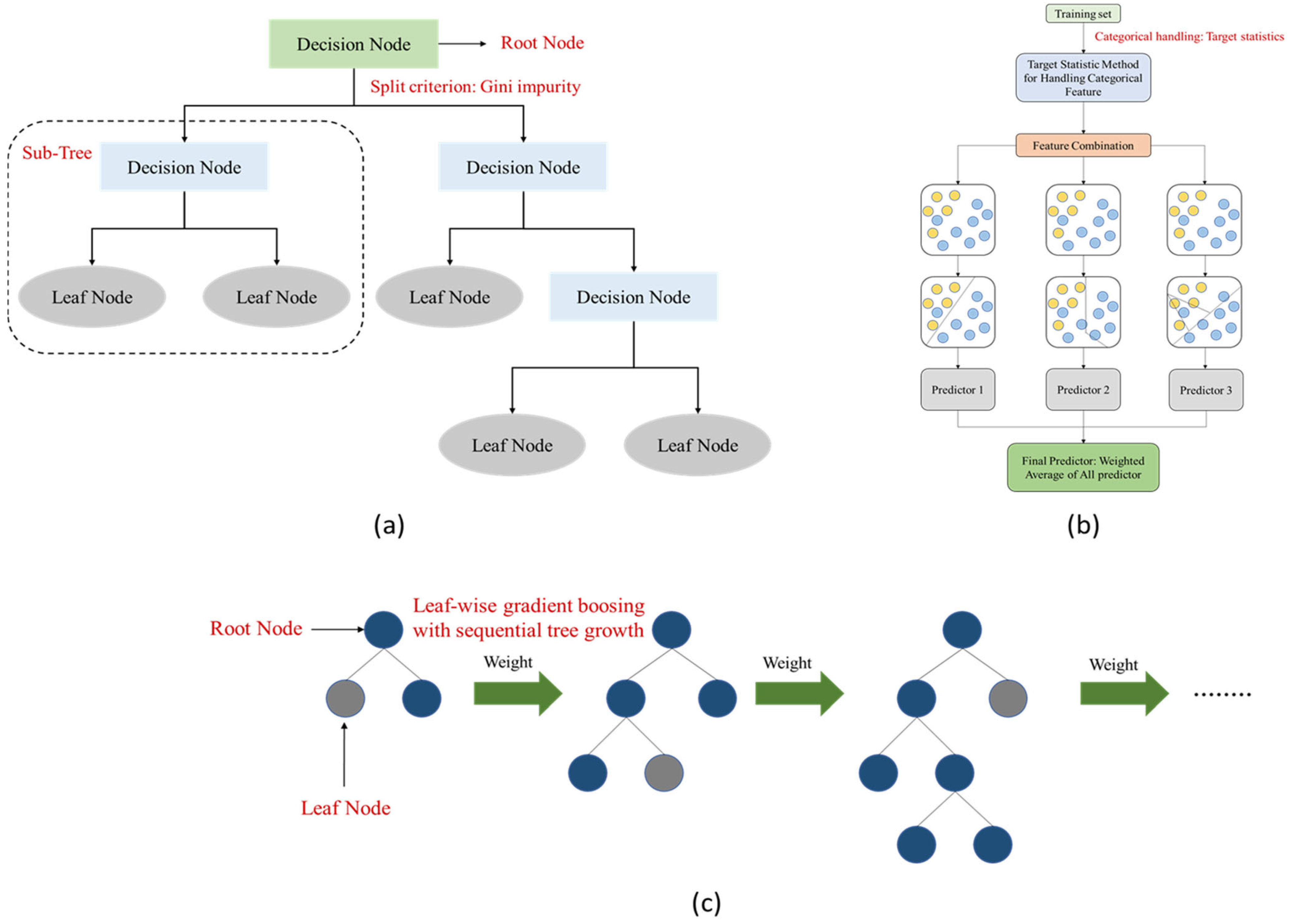
This study employed three machine learning models—Decision Tree (DT), CatBoost, and LightGBM—to estimate tractor performance. A structural overview of each model is presented in Figure 5. The entire dataset was randomly shuffled and evaluated using K-fold cross-validation to assess the generalization performance of each model. To ensure the reproducibility of the results, all random processes were controlled by setting a fixed random seed of 42.
The performance of the developed estimation models was evaluated using the following statistical metrics: coefficient of determination (R2), root mean square error (RMSE), mean absolute error (MAE), mean absolute percentage error (MAPE), and relative deviation (RD). MAPE expresses individual prediction errors as a percentage of the actual values, enabling intuitive interpretation, whereas RD compares RMSE with the mean actual value to provide a relative assessment of the overall error magnitude; therefore, both metrics were used in parallel. These metrics were calculated using Equations (3)–(7), as shown in the following formulas:
R 2   =   i =   1 i     =   N   ( y i     y a )     i   =   1 i   =   N   ( y i     y i ^ ) i = 1 i = N ( y i y a )
R M S E = 1 N i = 1 i = N y i ^ y i 2
M A E =   1 N i = 1 N y ^ i y i
M A P E = 1 N i = 1 i = N 1 y i ( y i y i ^ ) × 100 %
R D = R M S E M e a n   × 100 %
where y a is the mean measured tractor performance, y i is the ith measured tractor performance, and y i ^ is the ith estimated tractor performance.
In general, an R2 value greater than 0.70 is considered to indicate acceptable performance, while values in the range of 0.80–0.90 or higher are regarded as evidence of strong predictive ability in engineering and agricultural sciences [32]. RMSE is more meaningful when interpreted relative to the data range or mean rather than as an absolute value, and values less than 10% of the mean observed value are considered satisfactory accuracy in studies on agricultural machinery and soil–machine interactions [33].
Field-collected data used in this study were described using specific statistical parameters, including the maximum, minimum, average, standard deviation (SD), and coefficient of variation (CV). The CV was calculated using Equation (8):
C V =   S D A v e r a g e   × 100 %
Identifying overfitting during model development is critical as overfitting occurs when the model becomes overly tailored to the training data, resulting in poor estimation performance on new, unseen data. To assess overfitting, two additional metrics were used:
  • Train-to-test loss ratio (TTLR): This variable represents the ratio of the mean squared errors (MSE) of the test and training datasets. A TTLR of <1.5 indicates underfitting, while a TTLR of >1.5 indicates overfitting.
  • R2 Gap: This measures the difference between the R2 values of the training and test datasets. A large R2 Gap value suggests a strong likelihood of overfitting, implying the model performs significantly better on training data than test data.
The MSE, TTLR, and R2 Gap were determined using Equations (9)–(11).
M S E = 1 N   i = 1 i = N ( y i y ^ i ) 2
T T L R = M S E t e s t M S E t r a i n
R 2   G a p = |   R 2 t r a i n R 2 t e s t   |
where y i denotes the ith measured tractor performance and y i ^ denotes the ith estimated tractor performance.

2.3.4. Software

The estimation models were run on a workstation with a 64-bit Windows 11 Pro operating system equipped with a 4.8-GHz processor and 256 GB of memory. Model development was conducted in a Python 3.9-based environment using Google Colab (2025 version). Core machine learning libraries were utilized, including sci-kit, DT, CatBoost, and LightGBM.

2.3.5. Overall Process

Figure 6 presents the overall workflow of this study. First, the input variables were set as SMC, CI, and sand proportion, while the output variables were ET, EP, SR and AP. The data preprocessing stage involved a description of the data distribution and a data cleaning process. The dataset was then split into a training set (70%) and a test set (30%). In the tractor performance prediction model development stage, three machine learning algorithms—DT, CatBoost, and LightGBM—were applied. Hyperparameter optimization was conducted using Optuna in combination with 10-fold cross-validation on the training set. Model performance was evaluated using the test set (30%) based on eight evaluation metrics: R2, RD, RMSE, MSE, MAE, TTLR, MAPE, and R2 Gap. The best-performing model, CatBoost, was selected based on these evaluation results. For the sensitivity analysis, SHAP interpretation was performed using the best model (CatBoost) and a separate test subset (30%) to analyze the global importance and contribution of each input variable to the prediction of tractor performance.

3. Results

3.1. Effect of Soil Physical Properties on Tractor Performance

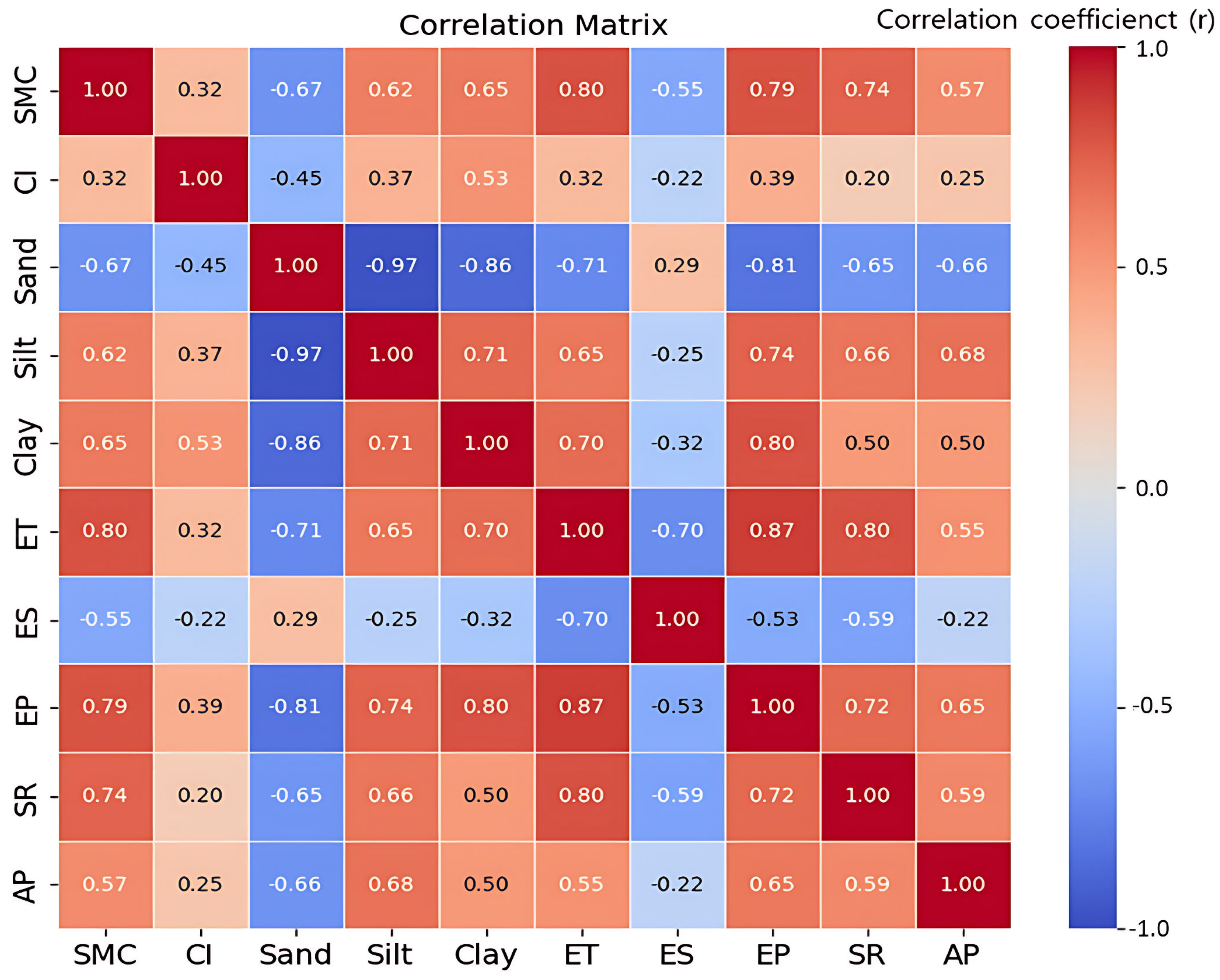
Figure 7 presents the correlation matrix between the key soil physical properties and tractor performance metrics. The correlation coefficients ranged from a maximum of 0.80 (between SMC and ET as well as clay and EP) to a minimum of −0.81 (between sand and EP). SMC showed the strongest overall correlation with tractor performance among the soil properties. Specifically, SMC had the greatest influence on ET, with a correlation coefficient of r = 0.80. For EP, the most influential properties in the descending order of effect were clay proportion (r = 0.80), SMC (r = 0.79), silt proportion (r = 0.74), CI (r = 0.39), and sand proportion (r = −0.81). The positive correlation between the clay proportion and EP suggested that as the clay proportion increased soil cohesion, a higher DF was required, which subsequently led to increased EP. SMC showed the highest correlation with SR (r = 0.74). Meanwhile, AP was most influenced by silt proportion (r = 0.68), followed by SMC (r = 0.57), clay proportion (r = 0.50), CI (r = 0.25), and sand proportion (r = −0.66). Correlation coefficients among sand, silt, and clay proportions were r = 0.71 (for silt and clay proportions), r = −0.86 (clay and sand proportions), and r = 0.97 (silt and sand proportions). These values indicate a comprehensive relationship among the particle types, where an increase in one type typically corresponded to a decrease in another. This interplay reflected the inherent regulatory mechanisms of soil physical properties, which influence soil aggregate structure and mechanical behavior.
Table 5 presents the performance of the developed regression models. The R2 Adj ranges from 0.104 to 0.771, indicating that each model explains between approximately 10.4% and 77.1% of the variance in tractor performance. Models A and B are univariate regression models that use single soil physical properties—SMC, CI, respectively. Model C is a bivariate model combining these two variables. Model D is a multivariate regression model that additionally incorporates the sand proportion as a soil texture variable, which led to improved estimation accuracy in most cases. For ET, Model D achieved the highest explanatory power with an R2 Adj of 0.693. Similarly, for EP, Model D showed superior performance with an R2 Adj of 0.771. These results suggest that including the sand proportion can enhance the accuracy of regression models. In contrast, for SR and AP, the improvement in explanatory power was relatively limited, even with the multivariate model, and the overall prediction accuracy remained low.
Table 6 displays the results of the ANOVA analysis for each regression model, including degrees of freedom (Df), sum of squares (SS), and mean squares (MS). In general, a higher F-value indicates that the regression model more effectively explains the variability in the dependent variable. Model A exhibited a higher F-value than Model B, suggesting stronger explanatory power. In contrast, Models C and D showed relatively lower F-values compared to Model A, indicating weaker explanatory capabilities. These results imply that SMC is more effective than CI in explaining tractor performance. The p-values, calculated based on the F-values and degrees of freedom, represent the probability that there is no significant relationship between the dependent and independent variables. All models demonstrated statistical significance at the p < 0.01 level.
The variance inflation factor (VIF) was used to diagnose multicollinearity, calculated as the reciprocal of tolerance. A VIF value closer to 1 indicates little to no multicollinearity among independent variables, while a value of 10 or higher suggests potential multicollinearity issues. In this study, the VIF values for all models ranged from 1.111 to 2.059, confirming that none of the models exhibited multicollinearity problems.

3.2. Machine Learning Model-Based Estimation of Tractor Performance

3.2.1. Engine Torque

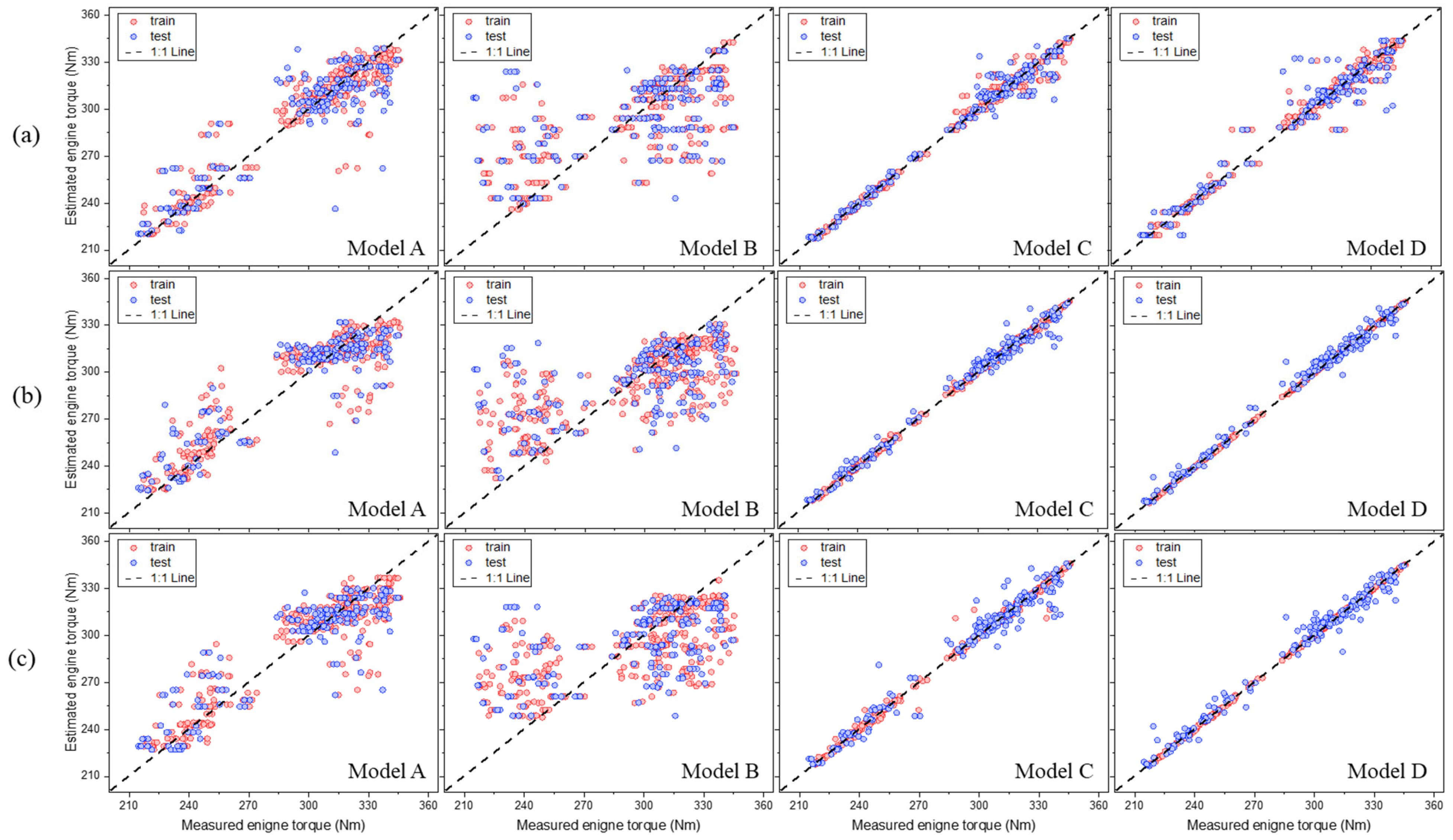
Figure 8 illustrates the results of ET estimation using different combinations of the input variables. The analysis revealed that Models C and D showed high estimation performance, with data points closely aligning with the reference line, whereas Models A and B exhibited greater data dispersion and relatively lower predictive accuracy. In addition, similar distributions were observed in both the training and test datasets, suggesting that the risk of overfitting was not significant. However, some deviations were noted in the high engine torque range, which may be attributed to the models’ limited ability to fully capture the nonlinearities of soil–machine interactions under heavy-load conditions.
Table 7 summarizes the performance of the three machine learning algorithms—DT, CatBoost, and LightGBM—in estimating ET. The models were evaluated using five metrics: R2, RMSE, MAE, MAPE, and RD. Model robustness and overfitting were assessed using the R2 Gap and TTLR metrics. Across all models, the R2 values ranged from 0.220 to 0.990, the RMSE ranged from 1.34 to 9.15 Nm, the MAE ranged from 1.34 to 9.46 Nm, MAPE ranged from 0.64% to 9.17, and the RD ranged from 1.24% to 11.06%. Model B exhibited the lowest R2 value, indicating limited estimation performance. In contrast, CatBoost-based model D achieved the highest estimation accuracy with R2 of 0.990, RMSE of 3.65 Nm, MAE of 2.80 Nm, MAPE of 0.96%, and RD of 1.24%.

3.2.2. Engine Power

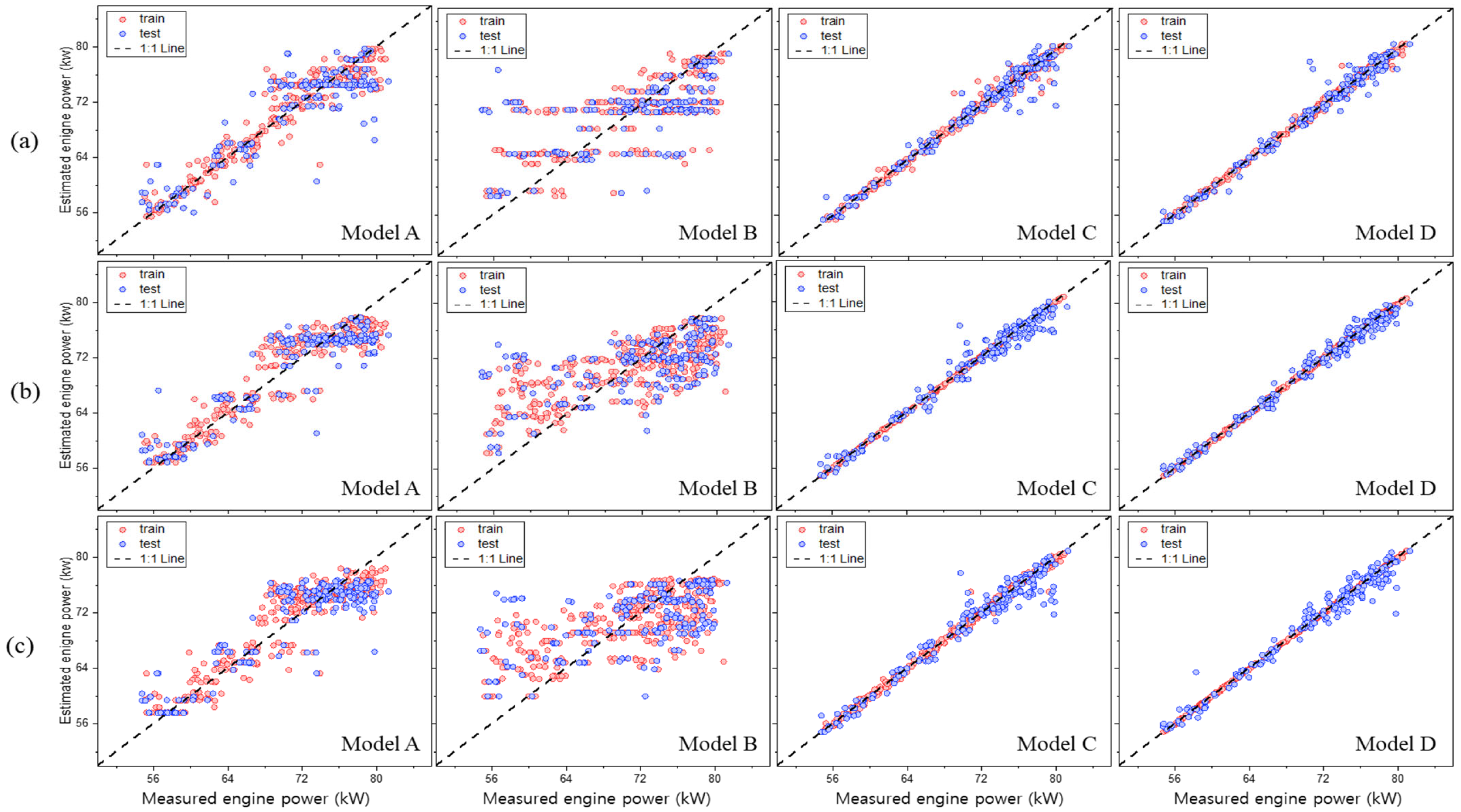
Figure 9 summarizes the performance metrics of the EP estimation models, showing the comparison of the measured and estimated EP values across different combinations of the input variables. The results demonstrated that alignment with the 1:1 reference line improved as the number of input variables increased. Models C and D exhibited data points that closely aligned with the 1:1 reference line across the entire output range, demonstrating high estimation performance and stability. In contrast, Models A and B showed instances of overestimation or underestimation in certain ranges. Additionally, Models C and D maintained a high level of consistency between the training and test datasets across the full output range, indicating that the risk of overfitting was not substantial.
Table 8 summarizes the performance metrics of the EP estimation models. The analysis revealed that all models, except model B, achieved R2 values of at least 0.728. Model A achieved an average R2 of 0.738. Meanwhile, model B exhibited the lowest performance, with an average R2 of 0.394. Model C showed a significantly improved average R2 of 0.932 compared to models A and B. When sand proportion was included in model D, the average R2 was 0.948. These findings indicate that using multiple input variables enhances the estimation performance compared to using a single variable. The overfitting assessment results showed that the R2 Gap was below 0.181 and the TTLR was below 1.94. However, the TTLR value for Model B was relatively higher compared to the other models, suggesting that when using Model B, techniques such as dropout, early stopping, and cross-validation should be applied to prevent overfitting.

3.2.3. Slip Ratio

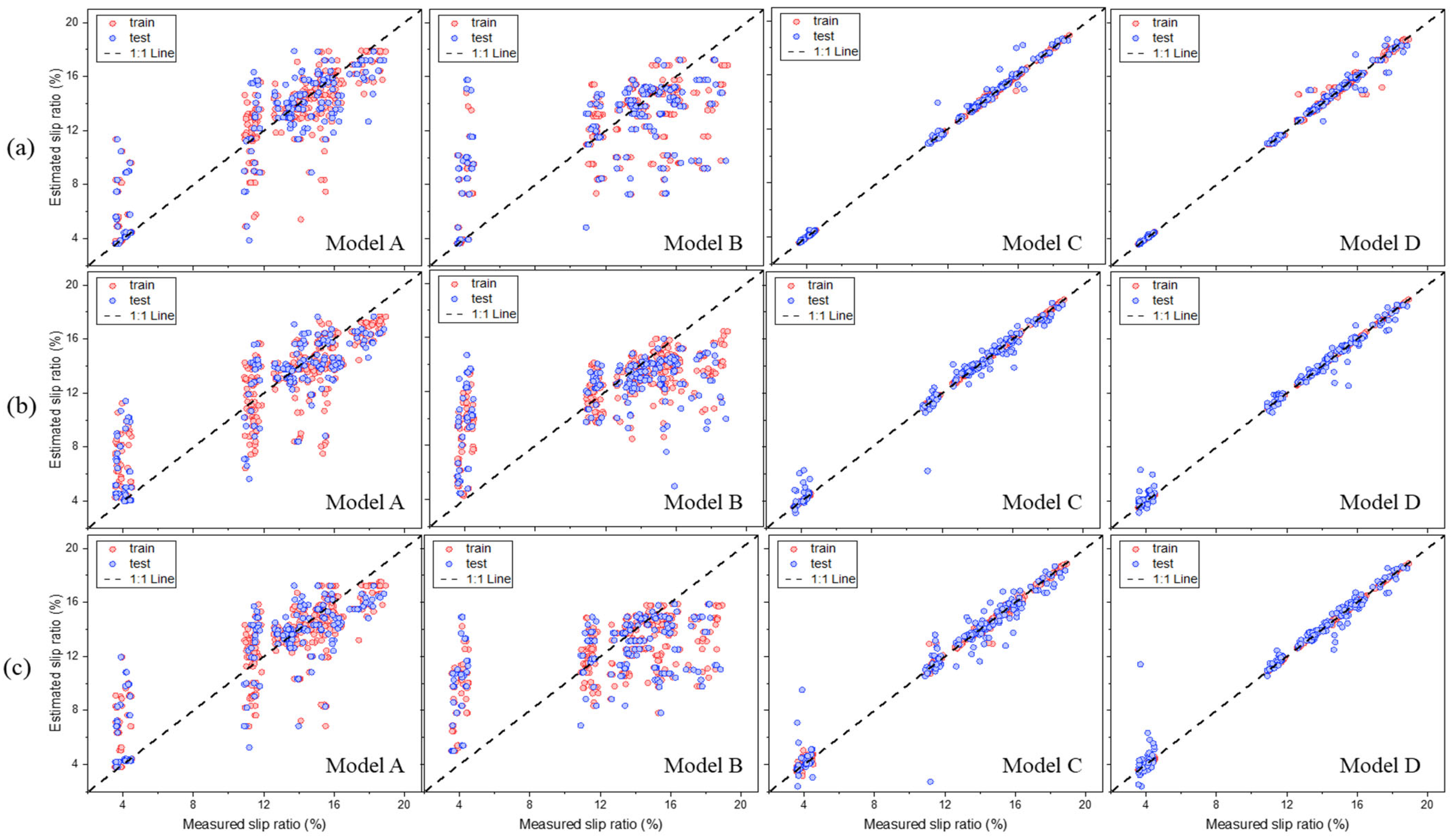
Figure 10 presents the results of the SR estimation models, comparing the measured and estimated SR values for each combination of input variables. Among the developed models, models C and D showed the closest alignment with the 1:1 reference line, indicating the highest estimation accuracy. In contrast, Models A and B exhibited greater data dispersion and showed a clear deviation from the reference line overall, resulting in relatively lower predictive performance. The errors were particularly pronounced in the low- and high-slip regions, which can be attributed to the inability of simple models to adequately capture the nonlinear nature of slip ratio influenced by multiple factors such as soil conditions, traction, and load.
Table 9 summarizes the performance metrics of each model. In particular, Model B, which utilized the CatBoost algorithm, achieved the highest accuracy with an R2 of 0.983, an RMSE of 0.61%, an MAE of 0.35%, a MAPE of 3.84%, and an RD of 2.97%. Although the MAPE for SR prediction was relatively high, this was due to the disproportionate influence of relative errors in sections where the actual values were small. Given that the absolute error metrics (RMSE and MAE) were very low, the prediction reliability is still considered high.

3.2.4. Axle Power

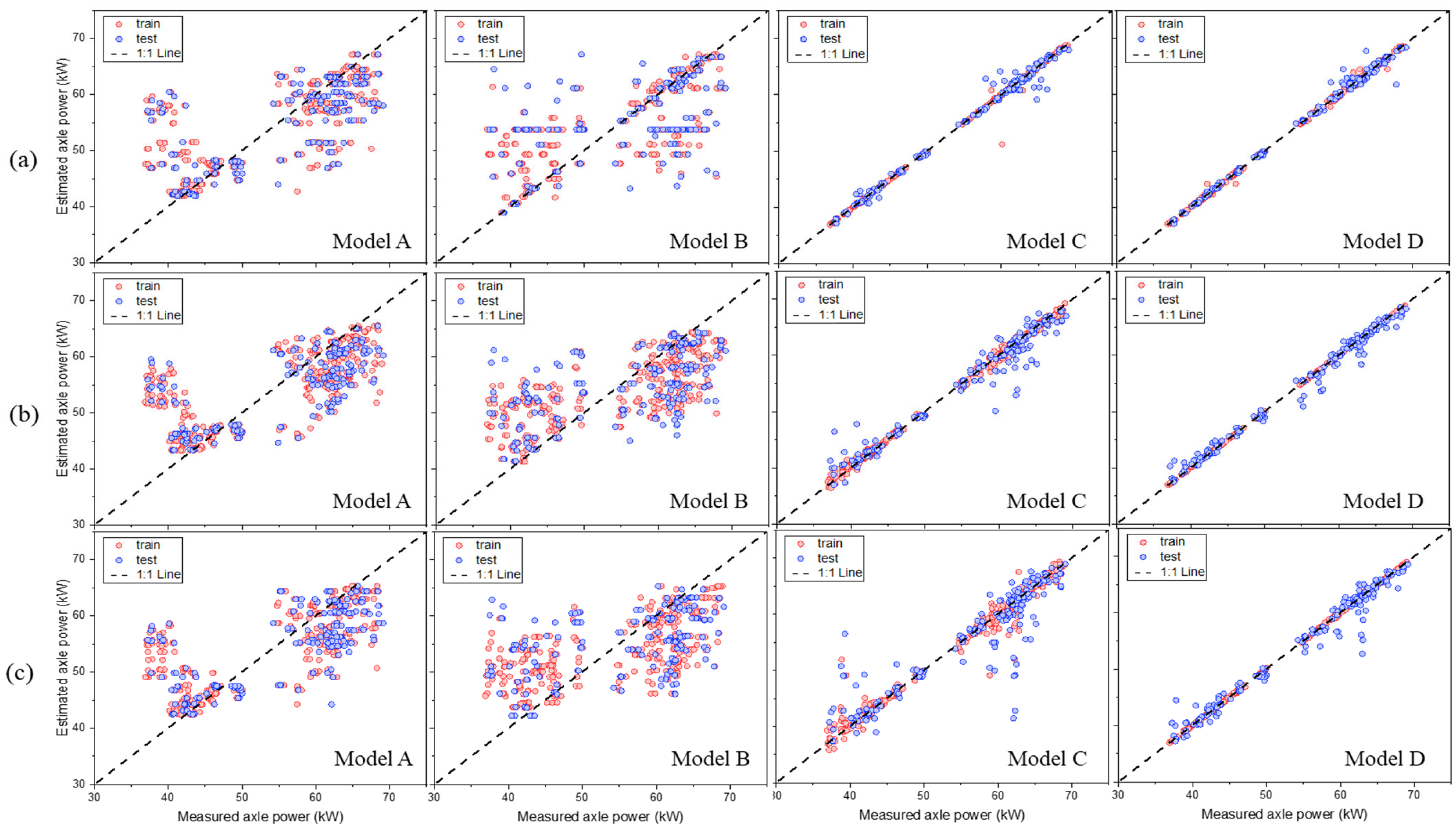
Figure 11 presents the results of the AP estimation models, comparing the measured and estimated AP values for each combination of input variables. Among the developed models, Model D showed the highest agreement with the 1:1 reference line. In addition, a general trend was observed in which the agreement with the reference line improved as the number of input variables increased. In the AP prediction, several data points in Model C were observed to deviate noticeably from the reference line. This indicates that using only SMC and CI has limitations in predicting AP, and that performance improves when soil texture is included as an additional input variable.
Table 10 summarizes the performance metrics of the AP estimation models. The analysis showed that the R2 values ranged from 0.120 to 0.959, RMSE values from 1.27 to 9.46 kW, MAE values from 0.88 to 7.98 kW, MAPE values from 1.55% to 9.30%, and RD values from 0.92% to 6.81%. Model B exhibited lower estimation performance compared to the other models, as indicated by its lower R2 value and higher RMSE, MAE, MAPE, and RD values. This suggests that using only CI as an input variable reduces estimation accuracy. Relying on a single input variable limits the model’s ability to capture the complex and variable conditions encountered in actual field operations. Therefore, incorporating multiple soil-related variables can provide a more comprehensive understanding of field conditions and improve the model’s estimation performance.

3.3. Combination and Evaluation of the Machine Learning-Based Estimation Models

Figure 12 presents the performance comparison of machine learning models for estimating tractor performance using R2 as the evaluation metric. For ET, Model B recorded the lowest R2 value, with DT and LightGBM showing particularly low values of 0.220 and 0.300, respectively. In contrast, Model C showed a substantial improvement in R2 values across all algorithms, with CatBoost achieving the highest value of 0.972. For EP, although Model B exhibited low R2 values, the other models demonstrated stable and reliable performance, with R2 values ranging from 0.728 to 0.980. Notably, in Model D, DT, CatBoost, and LightGBM achieved high accuracies of 0.898, 0.980, and 0.965, respectively. For SR, the R2 values ranged from 0.296 to 0.983, indicating considerable performance differences among the models. Model D achieved the highest estimation accuracy, with DT, CatBoost, and LightGBM recording R2 values of 0.919, 0.983, and 0.955, respectively. For AP, Model A showed lower accuracy compared to the other models, as using only SMC as an input variable was insufficient to capture the nonlinear characteristics of AP. In contrast, Model C achieved a significant improvement in estimation accuracy by incorporating two soil physical properties—SMC and CI—as input variables. This indicates that including a more diverse set of input variables contributes to improved estimation performance.
Overall, Model D utilizing CatBoost achieved the highest R2 values across ET, EP, SR, and AP estimations. This suggests that CatBoost, with its capability to effectively capture nonlinearity and interactions among variables, is well suited for addressing complex problems such as predicting agricultural machinery performance.
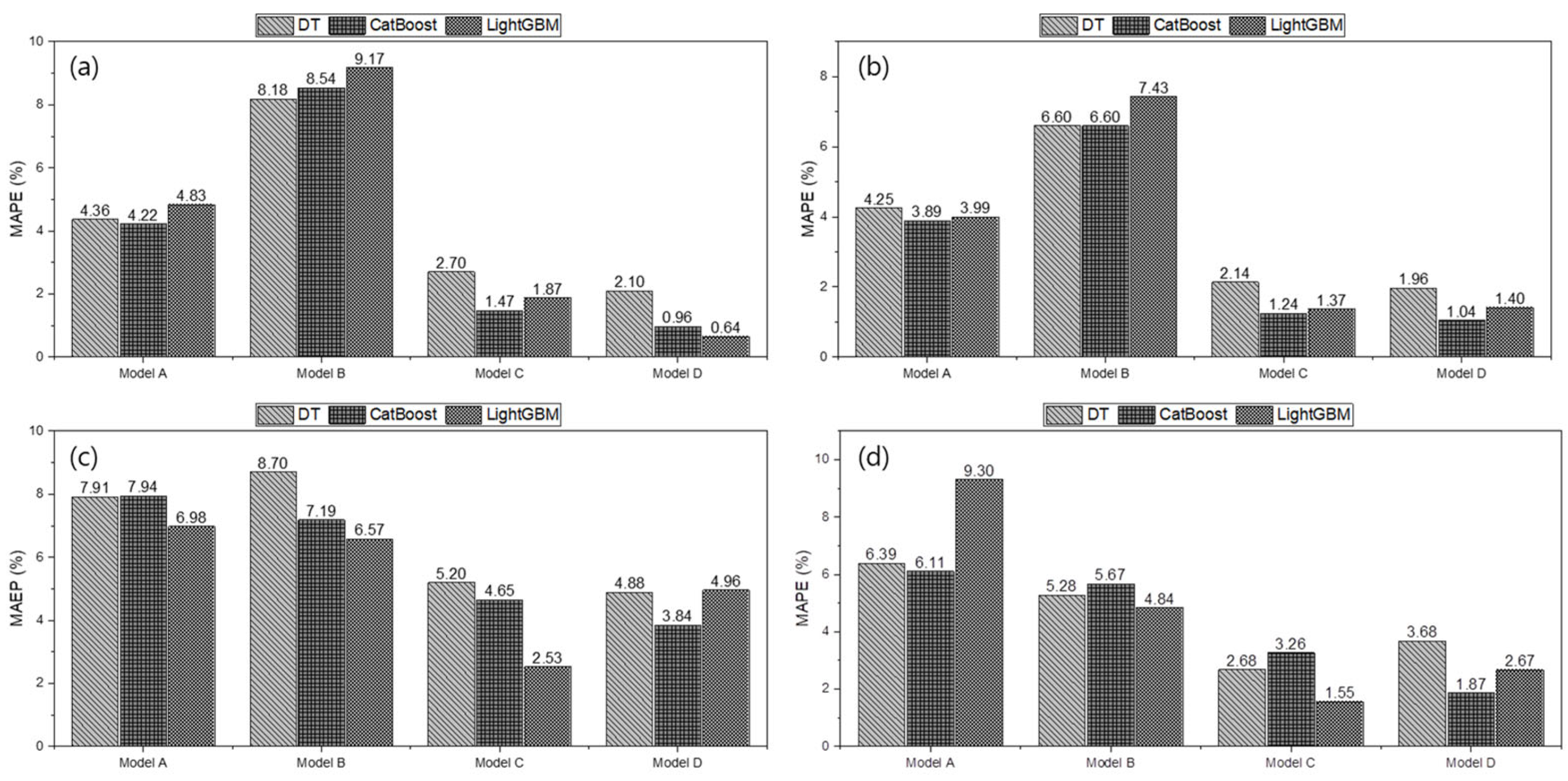
Figure 13 presents the comparison of prediction performance for three machine learning models in estimating ET, EP, SR, and AP using the MAPE metric. For ET, CatBoost and LightGBM in Model D achieved very low MAPE values of 0.96% and 0.64%, respectively, demonstrating the best performance. In contrast, Models A and B recorded MAPE values exceeding 4%, indicating that errors increased substantially when input variables were limited. For EP, all three algorithms (DT, CatBoost, and LightGBM) in Model B showed high MAPE values above 6.6%, whereas in Model D, the errors sharply decreased to below 2.0%. This demonstrates that prediction stability improves significantly when sufficient input variables are utilized. For SR, the performance differences among the models were the most pronounced. Models A and B exhibited high MAPE values in the range of 7–9%, whereas Model D substantially improved performance, with CatBoost and LightGBM achieving 3.84% and 4.96%, respectively. For AP, DT in Model A recorded the largest error at 9.30%, while CatBoost and LightGBM in Model D achieved very low errors of 1.87% and 2.67%, respectively, demonstrating stable performance.

3.4. Hyperparameter Optimization Results

Hyperparameter optimization was conducted using Optuna, focusing on key parameters that influence model complexity and learning behavior for each algorithm. For the DT model, the search space included max_depth ranging from 2 to 8, min_samples_split from 2 to 10, and min_samples_leaf from 1 to 5. The optimal configuration identified was max_depth = 8, min_samples_split = 8, and min_samples_leaf = 2. In the case of the CatBoost model, iterations were explored from 100 to 1000, learning_rate from 0.01 to 0.3, and depth from 3 to 10. The best-performing configuration was found to be iterations = 609, learning_rate = 0.160, and depth = 10. For the LightGBM model, the ranges considered were num_leaves between 20 and 100, learning_rate between 0.01 and 0.3, and n_estimators between 100 and 1000, with the optimal parameters determined as num_leaves = 75, learning_rate = 0.108, and n_estimators = 746. These optimal values were identified through Bayesian optimization using the Tree-Structured Parzen Estimator and contributed to improved model performance [34]. The summary of the results is presented in Table 11.

3.5. Shap Interpretation

To identify the key input features influencing the model’s prediction results and to enhance the interpretability and reliability of the model, SHAP sensitivity analysis was conducted. In this study, the analysis focused on global interpretation within the SHAP framework. SHAP analysis is based on an additive feature attribution method, where the explanation model g(z′) is represented as a linear function of binary features, as defined using Equation (12) [35].
g z = 0 + i = 1 M i z i
where M denotes the number of input features and i represents the Shapley value of feature i, the computation is outlined as follows. Let S denote the set of all features, and S i denote the set of features excluding feature i. P(S) refers to the power set of S, containing all possible subsets of S, while |A| represents the cardinality, or the number of elements, in set A. The Shapley value ( i ) for a particular feature i is calculated using Equation (13):
i   =   A P ( S i ) A ! · F · A 1 ! F !   [ f A i f ( A ) ]  
In this process, the sum is taken over all possible subsets A that exclude feature i, with F denoting the set of all features. The terms f (Ai) and f(A) represent the model’s output with and without the inclusion of feature i in subset A, respectively. This formula quantifies the marginal contribution of feature i across all possible combinations of features, offering a comprehensive view of the possible feature subsets.
Figure 14 presents the results of the sensitivity analysis conducted using the CatBoost-based prediction model. The relative importance of the three input variables—SMC, CI, and Sand—was evaluated for each prediction target based on SHAP values. For ET prediction, the SHAP values for SMC, CI, and Sand were 37.56, 33.26, and 29.18, respectively. SMC showed approximately 28.7% higher importance than Sand, indicating that soil moisture is the most influential factor in estimating ET. In the case of EP prediction, SMC had the highest SHAP value of 3.10, which was 17.0% and 162.7% greater than those of Sand and CI, respectively. This result emphasizes the dominant contribution of SMC to EP estimation. For SR prediction, SMC again had the greatest influence with a SHAP value of 1.92, followed by Sand (1.55) and CI (0.78). The importance of SMC was 23.9% higher than that of Sand, while CI had the lowest impact. In contrast, for AP prediction, Sand was the most important variable with a SHAP value of 6.02, which was 113.5% greater than that of SMC (2.82). This suggests that sand proportion plays a key role in predicting AP. The differences in feature importance among the performance indicators stem from the distinct physical mechanisms that each indicator reflects. ET, EP, and SR were all found to be highly sensitive to variations in soil moisture content, as soil moisture directly influences soil mechanical properties such as shear strength, cohesion, and internal friction angle. An increase in moisture reduces tire–soil friction, leading to higher slip ratios and consequently requiring the engine to deliver greater torque and power. In contrast, AP is largely governed by soil texture and shear resistance, with sand proportion playing a particularly critical role, as it alters soil drainage and strength characteristics, thereby directly affecting power transmission efficiency. Thus, while ET, EP, and SR are closely associated with soil moisture, AP is more strongly influenced by sand content.
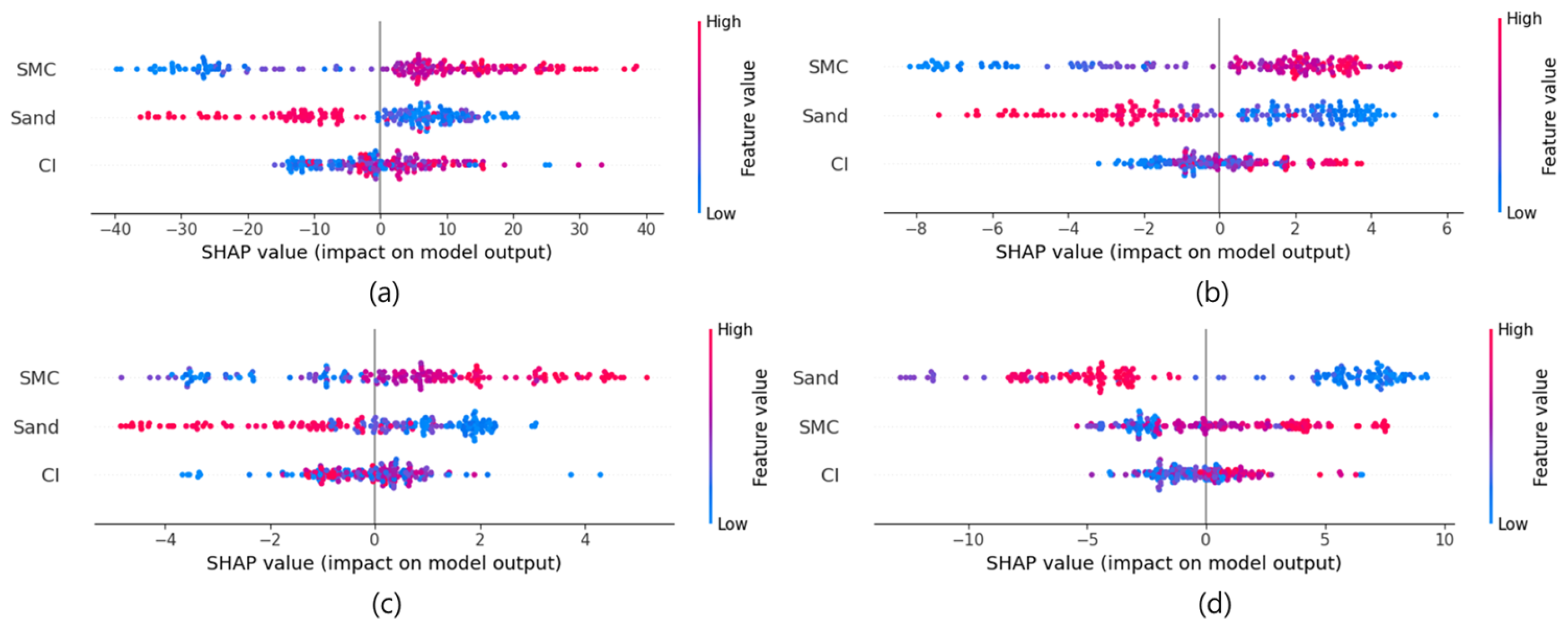
Figure 15 presents the SHAP summary plots of the CatBoost model, illustrating the contribution patterns of SMC, Sand, and CI for each prediction target. In the ET prediction, the SHAP values of SMC are broadly distributed and predominantly positive, indicating a tendency for higher soil moisture to increase the predicted values. Sand and CI exhibited both positive and negative effects, but their distributions were narrower compared to that of SMC. For EP and SR predictions, SMC also showed an increasing trend in SHAP values as feature values rose, suggesting a major contribution to the output. CI showed SHAP values largely concentrated around zero, indicating relatively consistent effects across samples. In the case of AP prediction, Sand displayed a wide range of SHAP values with a distinct positive pattern across various feature values, while SMC and CI showed more limited distributions within a narrower range.
Overall, the SHAP analysis results revealed patterns that align well with the known positive or negative correlations between each input variable and the corresponding prediction targets.

4. Discussion

In this study, machine learning-based models were developed to estimate key tractor performance indicators using various soil physical properties as input variables. Three algorithms—DT, CatBoost, and LightGBM—were applied, and model performance was evaluated across four input-variable combinations.
Overall, the results indicated that increasing the number of input variables generally improved estimation accuracy. Model D achieved the highest estimation accuracy across all performance indicators, with R2 values ranging from 0.840 to 0.990. In particular, CatBoost consistently recorded the highest R2 values among all algorithms, demonstrating its effectiveness in addressing complex estimation problems in agricultural environments. This can be attributed to CatBoost’s ability to effectively capture nonlinear relationships and interactions between variables, as well as its capabilities in handling categorical variables, automatic splitting, and built-in regularization techniques, which help prevent overfitting and maintain stable, high performance even with complex agricultural data [36]. LightGBM also demonstrated strengths in stable performance and fast training speed. In particular, compared with Random Forest, CatBoost and LightGBM are advantageous in terms of learning efficiency and memory usage, while compared with XGBoost, they offer benefits in automated handling of categorical variables and faster computational speed [37].
However, increasing the number of input variables also raised the complexity and computational cost of estimation. Model C, which used only a small number of input variables based on sensors capable of real-time measurement, demonstrated high performance, suggesting that it could serve as a practical and realistic solution for field applications. In contrast, Model B recorded the lowest performance, with R2 values ranging from 0.120 to 0.462, and showed particularly poor results in estimating SR and AP. This indicates that using CI alone as an input variable is insufficient to capture the complexity of soil–tractor interactions.
Among the three machine learning algorithms, CatBoost achieved the best overall estimation performance. DT offered advantages in interpretability and low computational cost but showed lower estimation accuracy. Overfitting was assessed using the R2 Gap and TTLR metrics, which ranged from 0.009 to 0.224 and from 1.00 to 1.94, respectively. These values indicate that, with few exceptions, most models achieved generalized estimation performance without significant overfitting.
This study addresses several limitations of previous research. Unlike earlier studies that primarily focused on SR or were conducted under restricted soil conditions, this work simultaneously estimated four key performance indicators—ET, EP, SR, and AP—thereby providing a more comprehensive framework for evaluating tractor performance. In terms of input variables, whereas prior studies often relied on a limited set, such as CI or SMC, this study proposed a multivariate estimation model that incorporates a wider range of soil physical properties, including soil texture composition. Nevertheless, some limitations remain, as data collection was confined to specific conditions, and the increased model complexity associated with additional input variables may lead to efficiency issues.
Future research should apply hyperparameter optimization and regularization techniques to further reduce overfitting. In addition, expanding data collection to include various soil types, such as clay, sandy loam, and silt loam, as well as diverse operating conditions, including plowing, rotary tillage, and harvesting, under different soil moisture levels and seasonal climatic variations, will further enhance the robustness and generalizability of the model. Furthermore, it is necessary to validate the model’s performance under extreme soil conditions, such as severe drought or excessive moisture, to more reliably ensure its adaptability in real agricultural environments.

5. Conclusions

In this study, a machine learning model was developed to predict key tractor performance indicators (ET, EP, SR, AP) based on soil physical properties. As a result, the CatBoost model demonstrated the best performance, recording an R2 value of 0.990 in ET prediction. This goes beyond previous studies that primarily relied on single variables, highlighting the academic significance of integrating multiple soil variables to improve the generalizability and reliability of tractor performance prediction. To develop such a model, it is necessary to first select test fields and measure various soil conditions, then choose a model appropriate for those conditions to predict the tractor’s key performance indicators. Furthermore, for practical implementation in the field, a systematic process of collecting soil condition data to be used as input variables is required. However, since this study was based on data collected from a specific region and limited soil conditions, there are inherent limitations in generalizing the findings to various soil types, climates, and working environments. Therefore, future research will focus on expanding the range and diversity of data and validating the model under diverse operating conditions to further strengthen its reliability and applicability.

Author Contributions

Conceptualization, Y.-J.K. and W.-S.K.; Methodology, S.-M.B. and S.-Y.B.; Software, S.-M.B. and S.-Y.B.; Validation, W.-S.K.; Formal analysis, S.-Y.G., S.-M.B. and S.-Y.B.; Investigation, S.-M.B. and S.-Y.B.; Resources, S.-M.B., S.-Y.B. and W.-S.K.; Data curation, S.-M.B., S.-Y.B. and W.-S.K.; Writing—original draft preparation, S.-Y.G. and W.-S.K.; Writing—review and editing, S.-Y.G. and W.-S.K.; Visualization, S.-Y.G.; Supervision, Y.-J.K. and W.-S.K.; Project administration, Y.-J.K.; Funding acquisition, Y.-J.K. All authors have read and agreed to the published version of the manuscript.

Funding

This research was supported by Korea Basic Science Institute (National research Facilities and Equipment Center) grant funded by the Ministry of Science and ICT (No. RS-2024-00404853).

Data Availability Statement

The raw data supporting the conclusions of this article will be made available by the authors on request.

Conflicts of Interest

The authors declare no conflicts of interest.

References

  1. Kim, J.-H.; Lee, C.-Y.; Cho, Y.-H.; Yu, Z.; Kim, K.-M.; Yang, Y.-J.; Nam, J.-S. Potato Farming in the United States and South Korea: Status Comparison of Cultivation Patterns and Agricultural Machinery Use. J. Biosyst. Eng. 2024, 49, 252–269. [Google Scholar] [CrossRef]
  2. Raikwar, S.; Tewari, V.K. Development of Transmission Control Algorithm for Power Shuttle Transmission System for an Agricultural Tractor. J. Biosyst. Eng. 2022, 48, 136–151. [Google Scholar] [CrossRef]
  3. Simikić, M.; Dedović, N.; Savin, L.; Tomić, M.; Ponjičan, O. Power Delivery Efficiency of a Wheeled Tractor at Oblique Drawbar Force. Soil Tillage Res. 2014, 141, 32–43. [Google Scholar] [CrossRef]
  4. Ahn, D.-V.; Kim, K.; Choi, K.; Lee, J.W.; Kim, J.-G.; Yu, J.; Kim, H.-S.; Seo, J.; Park, Y.-J. Effect of Clutch Control to Improve Launch Quality for a Power Shuttle Tractor during Launching. Comput. Electron. Agric. 2024, 224, 109235. [Google Scholar] [CrossRef]
  5. Kwon, D.; Ahn, D.-V.; Kim, J.-G.; Park, Y.-J. Effect Analysis of Motor Power Characteristics on the Energy Consumption of Dual Motor Driven Powertrain for Electric Tractor. J. Biosyst. Eng. 2024, 49, 465–475. [Google Scholar] [CrossRef]
  6. Rajabi-Vandecchali, M.; Abbaspour-Fard, M.H.; Rohani, A. Development of a Prediction Model for Estimating Tractor Engine Torque Based on Soft Computing and Low Cost Sensors. Measurement 2018, 121, 83–95. [Google Scholar] [CrossRef]
  7. Janulevičius, A.; Juostas, A.; Pupinis, G. Tractor’s Engine Performance and Emission Characteristics in the Process of Ploughing. Energy Convers. Manag. 2013, 75, 498–508. [Google Scholar] [CrossRef]
  8. Zhu, S.; Wang, L.; Zhu, Z.; Mao, E.; Chen, Y.; Liu, Y.; Du, X. Measuring Method of Slip Ratio for Tractor Driving Wheels Based on Machine Vision. Agriculture 2022, 12, 292. [Google Scholar] [CrossRef]
  9. Kara, S.; Karadirek, I.E.; Muhammetoglu, A.; Muhammetoglu, H. Real Time Monitoring and Control in Water Distribution Systems for Improving Operational Efficiency. Desalination Water Treat. 2016, 57, 11506–11519. [Google Scholar] [CrossRef]
  10. Kim, J.; Lee, J.; Kim, D.; Choi, C.; Lee, M.; Kim, H.S. Developing a Prediction Model (Heavy Rain Damage Occurrence Probability) Based on Machine Learning. J. Korean Soc. Hazard Mitig. 2019, 19, 115–127. [Google Scholar] [CrossRef]
  11. Kumari, A.; Reheman, H. Tillage Operation with a Tractor Drawn Rotavator Using an Embedded Advisory System for Minimizing Fuel Consumption. J. Biosyst. Eng. 2023, 48, 487–502. [Google Scholar] [CrossRef]
  12. Oduma, O.; Oluka, S.I.; Eze, P.C. Effect of Soil Physical Properties on Performance of Agricultural Field Machinery in South Eastern Nigeria. Agric. Eng. Int. CIGR J. 2018, 20, 25–31. [Google Scholar]
  13. Al-Shammary, A.A.G.; Caballero-Calvo, A.; Fernández-Gálvez, J. Evaluating the Performance of a Novel Digital Slippage System for Tractor Wheels Across Varied Tillage Methods and Soil Textures. Agriculture 2024, 14, 1597. [Google Scholar] [CrossRef]
  14. Siddique, A.A.; Baek, S.-M.; Baek, S.-Y.; Jeon, H.-H.; Park, J.-D.; Park, M.-J.; Yang, C.-W.; Park, M.J.; Kim, Y.-S.; Kim, W.-S.; et al. Effect of Motor Speeds on Traction Performance of a Single-Motor Electric Tractor at Various Gear Stages during Plow Tillage. Sci. Rep. 2023, 13, 56590. [Google Scholar] [CrossRef]
  15. Janulevičius, A.; Damanauskas, V. Prediction of Tractor Drive Tire Slippage under Different Inflation Pressures. J. Terramech. 2022, 101, 23–31. [Google Scholar] [CrossRef]
  16. Ge, J.; Peng, S.; Cao, C.; Fang, L.; Qin, K. Numerical Prediction of Tractive Performance of Track–Soil Interaction System through Different Grouser Heights. Eng. Agrícola 2022, 42, 19–24. [Google Scholar]
  17. Min, Y.-S.; Kim, Y.-S.; Lim, R.-G.; Kim, T.-J.; Kim, Y.-J.; Kim, W.-S. The Influence of Soil Physical Properties on the Load Factor for Agricultural Tractors in Different Paddy Fields. Agriculture 2023, 13, 2073. [Google Scholar] [CrossRef]
  18. Alhassan, E.A.; Olaoye, J.O.; Lukman, A.F.; Adekanye, T.A.; Abioye, O.M. Statistical Modelling of a Tractor Tractive Performance during Ploughing Operation on a Tropical Alfisol. Open Agric. 2024, 9, 20220282. [Google Scholar] [CrossRef]
  19. Al-Dosary, N.M.N.; Alnajjar, F.M.; Aboukarima, A.E.W.M. Estimation of Wheel Slip in 2WD Mode for an Agricultural Tractor during Plowing Operation Using an Artificial Neural Network. Sci. Rep. 2023, 13, 59975. [Google Scholar] [CrossRef]
  20. Angelucci, L.; Varani, M.; Pinet, F.; Martin, V.; Vertua, A.; Molari, G.; Mattetti, M. The Role of Tyres and Soil Conditions in Enhancing the Efficiency of Agricultural Tractors. Soil Tillage Res. 2025, 251, 106570. [Google Scholar] [CrossRef]
  21. Almaliki, S.A.; Himoud, M.S.; Muhsin, S.J. Mathematical Model for Evaluating Slippage of Tractor under Various Field Conditions. Basrah J. Agric. Sci. 2021, 34, 49–59. [Google Scholar] [CrossRef]
  22. Seifu, Y.; Hiresamhir, S.; Tole, S.; Yilak, A. Evaluation of Tractor Field Performance Using Visual Basics Programming for Agricultural Farm Lands. Am. J. Agric. Sci. Eng. Technol. 2023, 7, 25–35. [Google Scholar] [CrossRef]
  23. Al-Mastawi, K.E.; Dahham, G.A.; Yahya, L.M. Effects of Soil Moisture Content, Tire Inflation Pressure, and Tillage Speed on Tractive Performance of 2WD Tractor in Northern Iraq. Trans. Chin. Soc. Agric. Mach. 2022, 53, 409–418. [Google Scholar]
  24. Kim, W.S.; Kim, Y.J.; Baek, S.Y.; Baek, S.M.; Kim, Y.S.; Kim, Y.K.; Choi, I.S. Traction Performance Evaluation of a 78-kW-Class Agricultural Tractor Using Cone Index Map in a Korean Paddy Field. J. Terramech. 2020, 91, 285–296. [Google Scholar] [CrossRef]
  25. Shafaei, S.M.; Loghavi, M.; Kamgar, S. Feasibility of Implementation of Intelligent Simulation Configurations Based on Data Mining Methodologies for Prediction of Tractor Wheel Slip. Inf. Process. Agric. 2019, 6, 183–199. [Google Scholar] [CrossRef]
  26. Najafi, G.; Ghobadian, B.; Tavakoli, T.; Buttsworth, D.R.; Yusaf, T.F.; Faizollahnejad, M. Performance and Exhaust Emissions of a Gasoline Engine with Ethanol Blended Gasoline Fuels Using Artificial Neural Network. Appl. Energy 2009, 86, 630–639. [Google Scholar] [CrossRef]
  27. Al-Sager, S.M.; Almady, S.S.; Marey, S.A.; Al-Hamed, S.A.; Aboukarima, A.M. Prediction of Specific Fuel Consumption of a Tractor during the Tillage Process Using an Artificial Neural Network Method. Agronomy 2024, 14, 492. [Google Scholar] [CrossRef]
  28. TYM Co. TYM Tractors Official Website. TYM Official Website. Available online: https://tym.world (accessed on 15 September 2025).
  29. Spectrum Technologies Inc. FieldScout TDR 350 Soil Moisture Meter (Case Included). Spectrum Technologies Official Website. Available online: https://www.specmeters.com/FieldScout-TDR350-Soil-Moisture-Meter (accessed on 15 September 2025).
  30. Spectrum Technologies Inc. FieldScout SC900 Soil Compaction Meter. Spectrum Technologies Official Website. Available online: https://www.specmeters.com/FieldScout-SC900-Soil-Compaction-Meter (accessed on 15 September 2025).
  31. ASABE Standards EP542; Procedure for Using and Reporting Data Obtained with the Soil Cone Penetrometer. American Society of Agricultural and Biological Engineers: St. Joseph, MO, USA, 2019.
  32. Sima, N.Q.; Harmel, R.D.; Fang, Q.X.; Ma, L.; Andales, A.A. A modified F-test for evaluating model performance by including both experimental and simulation uncertainties. Environ. Model. Softw. 2018, 104, 236–248. [Google Scholar] [CrossRef]
  33. Tadić, V.; Radočaj, D.; Jurišić, M. Machine Learning Methods for Evaluation of Technical Factors of Spraying in Permanent Plantations. Agronomy 2024, 14, 1977. [Google Scholar] [CrossRef]
  34. Dhanka, S.; Maini, S. A Hybridization of XGBoost Machine Learning Model by Optuna Hyperparameter Tuning Suite for Cardiovascular Disease Classification with Significant Effect of Outliers and Heterogeneous Training Datasets. Int. J. Cardiol. 2024, 420, 132757. [Google Scholar] [CrossRef]
  35. Lundberg, S.M.; Lee, S. A Unified Approach to Interpreting Model Predictions. In Proceedings of the 31st Conference on Neural Information Processing Systems (NIPS), Long Beach, CA, USA, 4–9 December 2017. [Google Scholar]
  36. Hancock, J.T.; Khoshgoftaar, T.M. CatBoost for big data: An interdisciplinary review. J. Big Data 2020, 7, 94. [Google Scholar] [CrossRef]
  37. Ahn, J.M.; Kim, J.; Kim, K. Ensemble Machine Learning of Gradient Boosting (XGBoost, LightGBM, CatBoost) and Attention-Based CNN-LSTM for Harmful Algal Blooms Forecasting. Toxins 2023, 15, 608. [Google Scholar] [CrossRef]
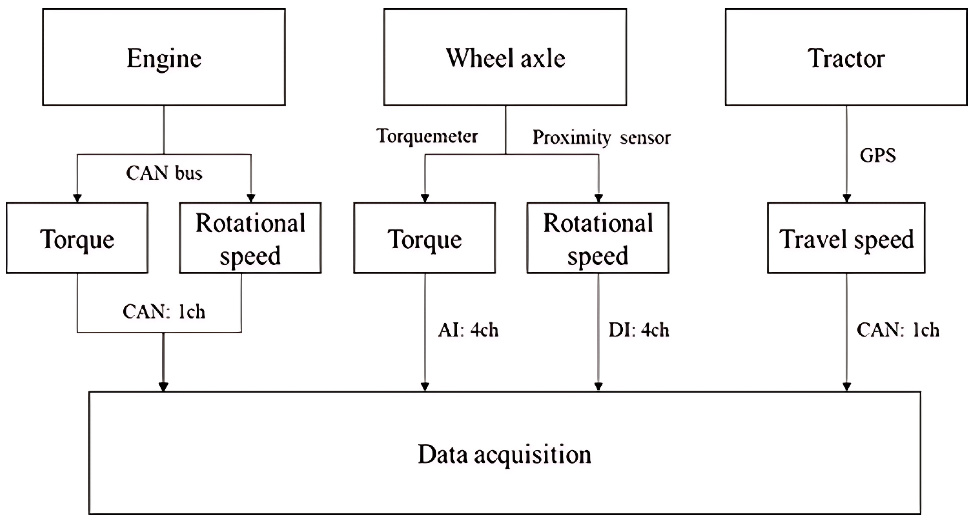
Figure 1. Schematic diagram of data measurement system.
Agronomy 15 02228 g001
Figure 2. Torque and proximity sensors installed on tractors.
Agronomy 15 02228 g002
Figure 3. Results of box plot analysis of soil physical property measured on field experiment sites (e.g., S1 refers to site 1): (a) soil moisture content (SMC), (b) cone index (CI), (c) sand, (d) silt, (e) clay.
Agronomy 15 02228 g003
Figure 4. Results of box plot analysis of tractor performance measured on field experiment sites (e.g., S1 refers to site 1): (a) engine torque, (b) engine speed, (c) engine power, (d) slip ratio, (e) axle power.
Agronomy 15 02228 g004
Figure 5. Overview of machine-learning models: (a) Decision Tree (DT), (b) CatBoost, (c) LightGBM.
Agronomy 15 02228 g005
Figure 6. Framework for machine learning-based tractor performance prediction and interpretation.
Agronomy 15 02228 g006
Figure 7. Correlation analysis results between soil physical properties and tractor performance data. Note: SMC: Soil moisture content (%); CI: Cone index (kPa); ET: Engine torque (Nm); ES: Engine speed (rpm); EP: Engine power (kW); SR: Slip ratio (%); AP: Axle power (kW).
Agronomy 15 02228 g007
Figure 8. Scatter plots of the estimated and estimated values for the engine torque: (a) DT, (b) CatBoost, and (c) LightGBM. Note: The 1:1 reference line represents perfect agreement between the observed and predicted values. The closer the data points are to this line, the better the predictive performance of the model is considered to be.
Agronomy 15 02228 g008
Figure 9. Scatter plots of the estimated and estimated values for the engine power: (a) DT, (b) CatBoost, and (c) LightGBM. Note: The 1:1 reference line represents perfect agreement between the observed and predicted values. The closer the data points are to this line, the better the predictive performance of the model is considered to be.
Agronomy 15 02228 g009
Figure 10. Scatter plots of the estimated and estimated values for the slip ratio: (a) DT, (b) CatBoost, and (c) LightGBM. Note: The 1:1 reference line represents perfect agreement between the observed and predicted values. The closer the data points are to this line, the better the predictive performance of the model is considered to be.
Agronomy 15 02228 g010
Figure 11. Scatter plots of the estimated and estimated values for the axle power: (a) DT, (b) CatBoost, and (c) LightGBM. Note: The 1:1 reference line represents perfect agreement between the observed and predicted values. The closer the data points are to this line, the better the predictive performance of the model is considered to be.
Agronomy 15 02228 g011
Figure 12. Performance comparison of three machine learning models using R2 for predicting (a) engine torque, (b) engine power, (c) slip ratio, (d) axle power.
Agronomy 15 02228 g012
Figure 13. Performance comparison of three machine learning models using MAPE for predicting (a) engine torque, (b) engine power, (c) slip ratio, (d) axle power.
Agronomy 15 02228 g013
Figure 14. Feature importance of the three different models based on mean absolute SHAP value: (a) engine torque, (b) engine power, (c) slip ratio, (d) axle power.
Agronomy 15 02228 g014
Figure 15. SHAP summary plot of the CatBoost model: (a) engine torque, (b) engine power, (c) slip ratio, (d) axle power.
Agronomy 15 02228 g015
Table 1. Specification of the soil measurement equipment used in this study.
ItemsSpecification
Soil moisture sensorMeasurement unit: percentage of volumetric water content (VWC)
Range: 0% VWC to saturation
Accuracy: ±3.0% VWC
Cone penetrometerMeasurement unit: cone index (kPa)
Range: 0–45 cm, 0–7000 kPa
Accuracy: ±1.25 cm and ±103 ka
Table 2. Field information of the experiment sites.
SiteField Size (m2)ProvinceCity
S16000Chungcheongnam-doSeosan
S26000Chungcheongnam-doSeosan
S34000Chungcheongnam-doCheongyang
S44000Chungcheongnam-doCheongyang
S53000Gyeonggi-doAnseong
S64000Gyeonggi-doAnseong
S76000Chungcheongnam-doDangjin
S84000Chungcheongnam-doDangjin
S94000Chungcheongnam-doDangjin
S104000Chungcheongnam-doDangjin
Table 3. Statistical analysis results of soil physical properties and engine performance indicators.
ItemsMax.Avg.Std.CV (%)
Soil physical propertySMC46.2431.325.6418
CI210489138343
Sand88.1851.924.2646.7
Silt62.7634.5917.4550.4
Clay34.1113.58.4862.8
Engine performance indicatorsET345.8293.83712.6
ES2567.52303.7122.35.3
EP81.3270.877.039.9
SR18.9412.174.5237.1
AP69.154.69.9718.3
Table 4. Combination of variables used for model development.
SiteField Size (m2)Location
S16000Chungcheongnam-do
S26000Chungcheongnam-do
S34000Chungcheongnam-do
S44000Chungcheongnam-do
S53000Gyeonggi-do
S64000Gyeonggi-do
S76000Chungcheongnam-do
S84000Chungcheongnam-do
S94000Chungcheongnam-do
S104000Chungcheongnam-do
Table 5. Regression model for estimating tractor performance.
OutputModelRegression ModelR2R2 AdjS.E.
Engine torqueAET = 5.23SMC + 129.73390.6370.63622.3
BET = 0.0313CI + 265.85010.1050.10435.1
CET = 5.07SMC + 0.00768CI + 128.05910.6430.64222.2
DET = 3.82SMC − 0.000800CI − 0.499Sp + 200.84670.6950.69320.5
Engine powerAEP = 0.987SMC + 39.96250.6270.6274.30
BEP = 0.00724CI + 64.42650.1550.1546.47
CEP = 0.924SMC + 0.00292CI + 39.32510.6500.6494.17
DEP = 0.558SMC + 0.000451CI − 0.145Sp + 60.54720.7730.7714.17
Slip ratioASR = 0.590SMC − 6.31140.5420.5423.06
BSR = 0.00238CI + 10.04870.0410.0394.43
CSR = 0.599SMC − 0.000415CI − 6.22100.5440.5423.06
DSR = 0.441SMC − 0.00148CI − 0.0627Sp + 2.92930.5990.5972.87
Axle powerAAP = 1.000SMC + 23.12410.3230.3228.21
BAP = 0.00658CI + 48.74210.0640.0629.66
CAP = 0.960SMC + 0.00210CI + 22.66690.3290.3278.19
DAP = 0.402SMC − 0.00168CI − 0.221Sp + 54.97210.4700.4687.28
Table 6. ANOVA results for each regression model.
OutputModelDegrees of Freedom (Df)Sum of Squares (SS)Mean Squares (MS)F-Valuep-ValueVariableToleranceVariance Inflation Factor (VIF)
Engine torqueARegression1523,869.8523,869.81049.70.000 *SMC
Residual9298,450.1499.1
BRegression186,400.786,400.770.20.000 *CI
Residual9735,919.11230.6
CRegression2528,537.6264,268.8537.00.000 *SMC0.9901.111
Residual8293,782.3492.1CI0.9901.111
DRegression3571,231.4190,410.5452.0000.000 *SMC
CI
Sand
0.550
0.794
0.486
1.817
1.260
2.059
Residual7251,088.4421.3
Engine powerARegression118,598.718,598.71006.5000.000 *SMC
Residual911,049.718.5
BRegression14602.04602.0109.9000.000 *CI
Residual925,046.341.9
CRegression219,274.89637.4554.6000.000 *SMC0.9001.111
Residual810,373.617.4CI0.9001.111
DRegression322,904.17634.7674.7000.000 *SMC
CI
Sand
0.550
0.794
0.486
1.817
1.260
2.059
Residual76744.211.3
Slip ratioARegression16648.46648.4708.9000.000 *SMC
Residual95608.69.4
BRegression1497.9497.925.3000.000 *CI
Residual911,759.119.7
CRegression26662.03331.0355.4290.000 *SMC0.9001.111
Residual85594.99.4CI0.9001.111
DRegression37336.72445.6296.2000.000 *SMC
CI
Sand
0.550
0.794
0.486
1.817
1.260
2.059
Residual74920.38.3
Axle powerARegression119,287.019,287.0285.8280.000 *SMC
Residual940,351.767.5
BRegression13801.73801.740.7150.000 *CI
Residual955,837.093.4
CRegression219,634.99817.5146.5120.000 *SMC0.9001.111
Residual840,003.867.0CI0.9001.111
DRegression328,044.99348.3176.4000.000 *SMC
CI
Sand
0.550
0.794
0.486
1.817
1.260
2.059
Residual731,593.853.0
* Significant at p < 0.01.
Table 7. Performance evaluation of the machine learning models in estimating engine torque.
ItemsR2R2 GapRMSE (Nm)TTLRMAE (Nm)MAPE (%)RD (%)
TrainTestTrainTestTrainTestTrainTestTrainTest
ADT0.8340.7470.0885.176.311.495.826.963.694.365.176.22
CatBoost0.8830.7800.1035.546.781.508.709.462.984.224.276.04
LightGBM0.8220.7030.1195.737.821.866.477.333.954.835.366.73
BDT0.4110.2200.1928.609.151.135.556.677.448.189.7410.92
CatBoost0.5320.3470.1855.516.591.435.906.717.218.548.6910.73
LightGBM0.4240.3000.1244.305.551.666.406.438.109.179.6411.06
CDT0.9630.8480.1157.188.201.314.678.001.602.702.454.82
CatBoost0.9990.9720.0271.151.341.370.931.341.321.471.392.15
LightGBM0.9910.9490.0433.454.231.502.062.510.721.871.172.80
DDT0.9610.9150.0467.288.061.233.856.231.322.102.483.76
CatBoost0.9990.9900.0093.303.651.222.252.800.860.961.101.24
LightGBM0.9990.9680.0315.325.651.133.724.680.260.641.452.27
Table 8. Performance evaluation of the machine learning models in estimating engine power.
ItemsR2R2 GapRMSE (kW)TTLRMAE (kW)MAPE (%)RD (%)
TrainTestTrainTestTrainTrainTestTestTrainTest
ADT0.8670.7280.1392.502.871.321.823.012.544.253.535.45
CatBoost0.8510.7490.1022.713.531.702.162.773.063.893.834.97
LightGBM0.8190.7370.0822.993.611.462.342.843.323.994.225.08
BDT0.5910.4100.1814.465.341.432.884.514.236.606.298.98
CatBoost0.5620.3940.1684.535.781.633.504.505.156.606.408.14
LightGBM0.4990.3770.1234.946.471.723.745.125.477.436.969.17
CDT0.9500.8770.0731.622.251.941.021.571.422.142.303.13
CatBoost0.9990.9670.0321.091.281.390.680.890.971.240.131.80
LightGBM0.9960.9520.0451.431.491.080.290.980.421.371.612.10
DDT0.9620.8980.0641.341.491.230.851.371.171.961.883.27
CatBoost0.9990.9800.0190.991.001.010.770.720.911.041.131.41
LightGBM0.9990.9650.0341.211.381.301.161.991.231.401.301.95
Table 9. Performance evaluation of the machine learning models in estimating the slip ratio.
ItemsR2R2 GapRMSE (%)TTLRMAE (%)MAPE (%)RD (%)
TrainTestTrainTestTrainTrainTestTestTrainTest
ADT0.7020.5620.1402.482.961.421.792.306.727.916.506.94
CatBoost0.7810.6420.1392.122.671.581.592.087.617.947.587.64
LightGBM0.8080.6350.1731.992.701.841.372.016.536.986.476.85
BDT0.5340.4620.0723.114.041.692.072.778.188.706.887.29
CatBoost0.5830.3270.2572.943.621.522.102.596.787.195.476.94
LightGBM0.4850.2960.1893.273.701.282.402.716.786.577.209.59
CDT0.9380.8220.1161.111.341.450.420.764.865.203.095.24
CatBoost0.9990.9770.0220.570.701.530.360.384.474.654.465.87
LightGBM0.9970.9280.0691.241.241.000.540.631.662.531.962.54
DDT0.9970.9190.0781.251.341.140.110.463.924.882.063.95
CatBoost0.9990.9830.0160.520.611.380.220.353.083.842.182.97
LightGBM0.9980.9550.0440.981.001.040.510.544.464.961.452.18
Table 10. Performance evaluation of the machine learning models in estimating axle power.
ItemsR2R2 GapRMSE (kW)TTLRMAE (kW)MAPE (%)RD (%)
TrainTestTrainTestTrainTrainTestTestTrainTest
ADT0.4240.3880.0367.617.691.025.565.736.246.393.983.98
CatBoost0.5370.4100.1276.827.551.234.995.626.086.114.534.72
LightGBM0.6210.5020.1206.178.211.774.305.768.639.304.344.93
BDT0.2400.1200.1208.719.281.147.487.984.815.286.036.81
CatBoost0.5350.3100.2246.828.841.685.667.115.195.674.546.01
LightGBM0.4230.3860.0367.599.461.556.267.694.394.843.974.13
CDT0.8490.7430.1063.884.731.481.683.003.392.685.075.46
CatBoost0.9990.8890.1103.213.311.070.171.520.313.262.383.13
LightGBM0.9890.8310.1584.074.091.011.572.291.111.551.952.57
DDT0.9580.8400.1182.062.281.230.931.671.873.683.764.13
CatBoost0.9990.9590.0401.111.271.320.790.881.171.873.203.63
LightGBM0.9990.9240.0752.212.681.470.141.282.282.670.380.92
Table 11. Selected hyperparameter combinations for the machine learning models used to estimate the tractor performance.
DTCatBoostLightGBM
max_depth: 8number of iterations: 609num_leaves: 75
min_samples_split: 8learning_rate: 0.160learning_rate: 0.108
min_samples_leaf: 2depth: 10n_estimators: 746
Disclaimer/Publisher’s Note: The statements, opinions and data contained in all publications are solely those of the individual author(s) and contributor(s) and not of MDPI and/or the editor(s). MDPI and/or the editor(s) disclaim responsibility for any injury to people or property resulting from any ideas, methods, instructions or products referred to in the content.