High-Resolution 3D Reconstruction of Individual Rice Tillers for Genetic Studies

Abstract

The architecture of rice tillers plays a pivotal role in yield potential, yet conventional phenotyping methods have struggled to capture these intricate three-dimensional (3D) structures with high fidelity. In this study, a 3D model reconstruction method was developed specifically for rice tillers to overcome the challenges posed by their slender, feature-poor morphology in multi-view stereo-based 3D reconstruction. By applying strategically designed colorful reference markers, high-resolution 3D tiller models of 231 rice landraces were reconstructed. Accurate phenotyping was achieved by introducing ScaleCalculator, a software tool that integrated depth images from a depth camera to calibrate the physical sizes of the 3D models. The high efficiency of the 3D model-based phenotyping pipeline was demonstrated by extracting the following seven key agronomic traits: flag leaf length, panicle length, first internode length below the panicle, stem length, flag leaf angle, second leaf angle from the panicle, and third leaf angle. Genome-wide association studies (GWAS) performed with these 3D traits identified numerous candidate genes, nine of which had been previously confirmed in the literature. This work provides a 3D phenomics solution tailored for slender organs and offers novel insights into the genetic regulation of complex morphological traits in rice.

1. Introduction

Rice (Oryza sativa L.) is a staple food crop that sustains over half of the global population, making its yield and adaptability critical to food security. According to the 2023 FAOSTAT release, global paddy-rice production reached approximately 800 million tonnes, cultivated on some 168 million hectares of cropland [1]. As one of the key determinants of rice productivity, the tiller is a specialized, slender, and feature-poor branch that directly influences light interception efficiency, panicle formation, and grain yield [2,3]. Poor tiller architecture or morphology can induce lodging, resulting in substantial grain yield declines [4].

There have been efforts to better understand the phenotypic characteristics of rice tillers to overcome challenges. First, traditional phenotyping methods rely on manual measurements, which are labor-intensive and error-prone [5,6]. Second, two-dimensional (2D) image-based methods have been widely used by measuring length and angles. However, 2D methods are inherently limited by viewpoint dependence and projection distortion, limiting their reliability for three-dimensional (3D) morphological characterization [7,8]. For example, prior attempts to quantify maize leaf angles using 2D imaging have consistently encountered these methodological constraints [9,10]. Furthermore, 2D imaging methods fundamentally lack the capacity to capture complex 3D architecture [11], resulting in incomplete morphological assessments of rice tillers. Third, 3D reconstruction has been recently adopted to investigate rice phenotypes for the whole plant, but self-occlusion is a significant challenge [12,13,14]. In particular, rice tillers grow closely together, and the inner leaves are stacked on top of one another. This makes it difficult for researchers to extract phenotypes of fine-scale organs, particularly those of individual tillers, from whole plant 3D models.

Recent advancements in 3D reconstruction methods have significantly improved organ-level phenotyping, especially for analyzing the panicle structure of cereal tillers. First, multi-view stereo (MVS) technique reconstructs 3D structures by identifying and triangulating matching features across overlapping 2D images captured from different views [15,16,17]. For example, the PI-Plat platform utilizes a rotational camera setup and multi-view stereo (MVS) techniques to generate 3D models of rice panicles, extracting agronomic traits like volume and color [18]. Additionally, a follow-up study of PI-Plat expanded the trait set to digital descriptors including projected area, voxel count, and color intensity [19]. Second, Neural Radiance Fields (NeRF) is a deep learning-based approach that generates 3D reconstructions by learning a continuous volumetric representation from multiple 2D images [20]. For instance, the PanicleNeRF system integrated Neural Radiance Fields (NeRF) with image segmentation to enable detailed panicle modeling in the field using smartphone images [21]. Third, a sensor-based structured-light approach, Panicle-3D, delivers accurate segmentation and dense point-cloud generation for panicle analysis [22]. Robust feature matching is a prerequisite for both MVS and NeRF pipelines, each of which relies on Structure-from-Motion (SfM) to estimate camera poses and recover the intrinsic and extrinsic parameters required for 3D reconstruction. Nevertheless, the slender and feature-poor structure of rice tillers limits reliable feature matching in SfM, often resulting in fragmented models or pose estimation failures.

In light of these constraints, an MVS-based pipeline remains the most practical and scalable solution for the application [23,24]. Recent work has shown that a smartphone-based MVS workflow, when coupled with a generalized regression neural network, can non-destructively retrieve 11 soybean traits with errors of 3%, demonstrating the accuracy and affordability of commodity camera phenotyping [25]. Another study developed the compact MVS-Pheno V2 platform, whose rotating cameras acquire multi-view images to reconstruct sub-millimeter 3D point clouds of individual seedlings and automatically extract traits such as plant height, leaf area, and shoot volume [26]. An MVS-based pipeline requires only commodity cameras, yields high-resolution models at low cost, and when each tiller is imaged from all viewpoints in a controlled scene eliminates occlusion while capturing even the innermost leaves. The lack of intrinsic features can be overcome by introducing high-contrast reference markers at multiple viewpoints [27]; the colorful patterned backdrop used here supplies a dense grid of reliable keypoints, greatly improving SfM pose estimation for otherwise textureless stems.

The objective of this study is to develop a reconstruction method for 3D modeling of rice tillers, which are characterized by their slender and feature-poor morphology. While previous research has primarily focused on panicles, organs that are more robust and feature-rich, there are currently no MVS-based datasets available for rice tillers. To address this gap, we employed an MVS remote sensing approach combined with a SfM algorithm to generate high-resolution, actual-scale 3D models of individual rice tillers. The accuracy of the reconstructed models was assessed by comparing morphological traits derived from the 3D models with manual measurements. Furthermore, the utility of these 3D tiller models was demonstrated by integrating genotype and phenotype data extracted from the same rice population for genome-wide association analysis (GWAS). Collectively, this study presents a practical and scalable toolkit for phenotyping slender plant organs.

2. Materials and Methods

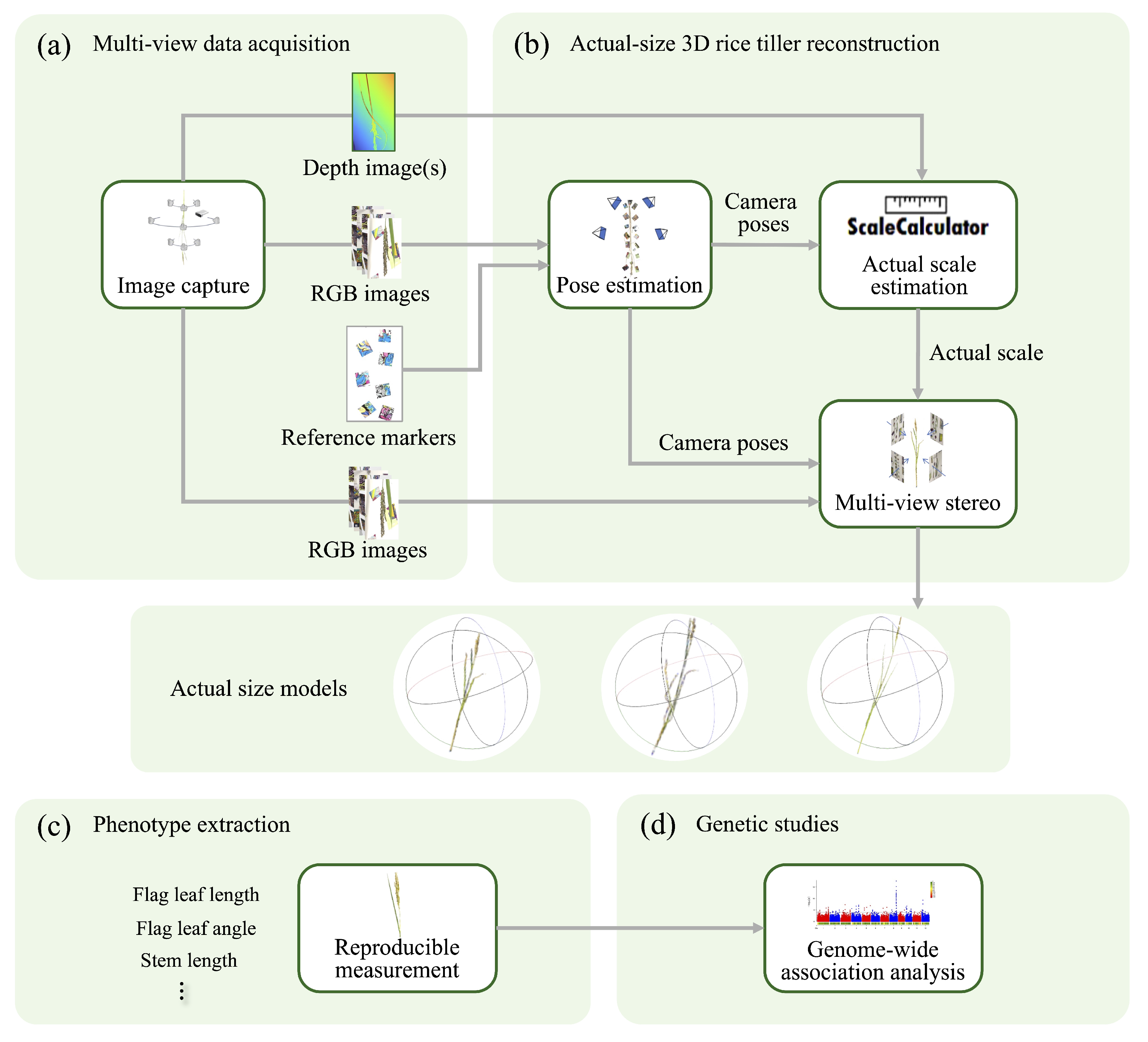
2.1. Overview of 3D Tiller Reconstruction for Genetic Study

The workflow consisted of four key steps to conduct genetic analysis of morphological traits based on 3D tiller models (Figure 1). The 3D reconstruction was implemented using the open source framework OSTRA [28], which was based on a multi-view stereo (MVS) approach and required multiple images captured from various viewpoints at different distances.

Rice tiller images were captured with a smartphone from multiple perspectives, with colorful reference markers in the background to improve pose estimation accuracy. One or more depth images from a depth camera were acquired to estimate parameters for actual-size adjustment. A custom tool, ScaleCalculator, was developed to recover the 3D models generated through MVS and to reconstruct actual-size 3D models. The resulting models underwent morphological analysis that included measurements of seven phenotypes: flag leaf length, panicle length, first internode length below the panicle, stem length, flag leaf angle, second leaf angle from the panicle, and third leaf angle from the panicle. Finally, genome-wide association analysis (GWAS) was conducted on these phenotypic traits to explore their genetic associations.

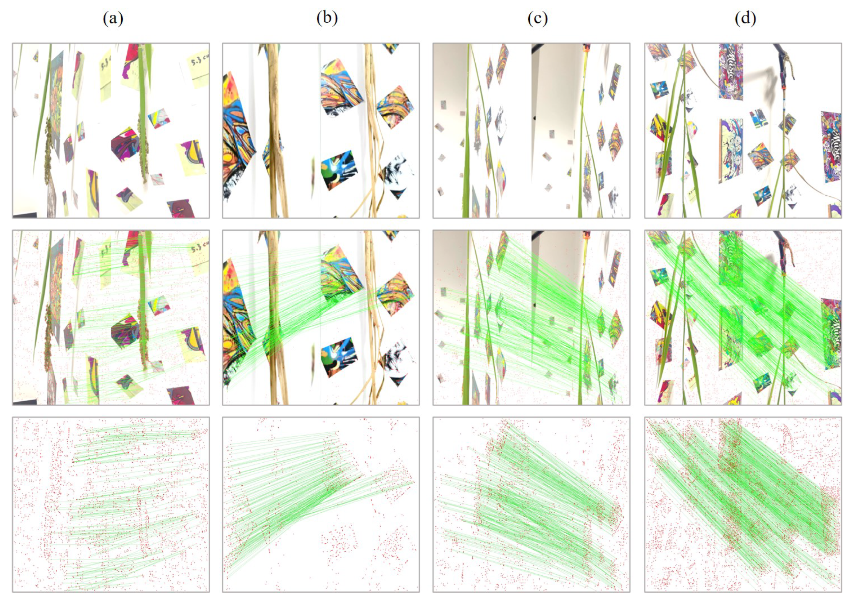
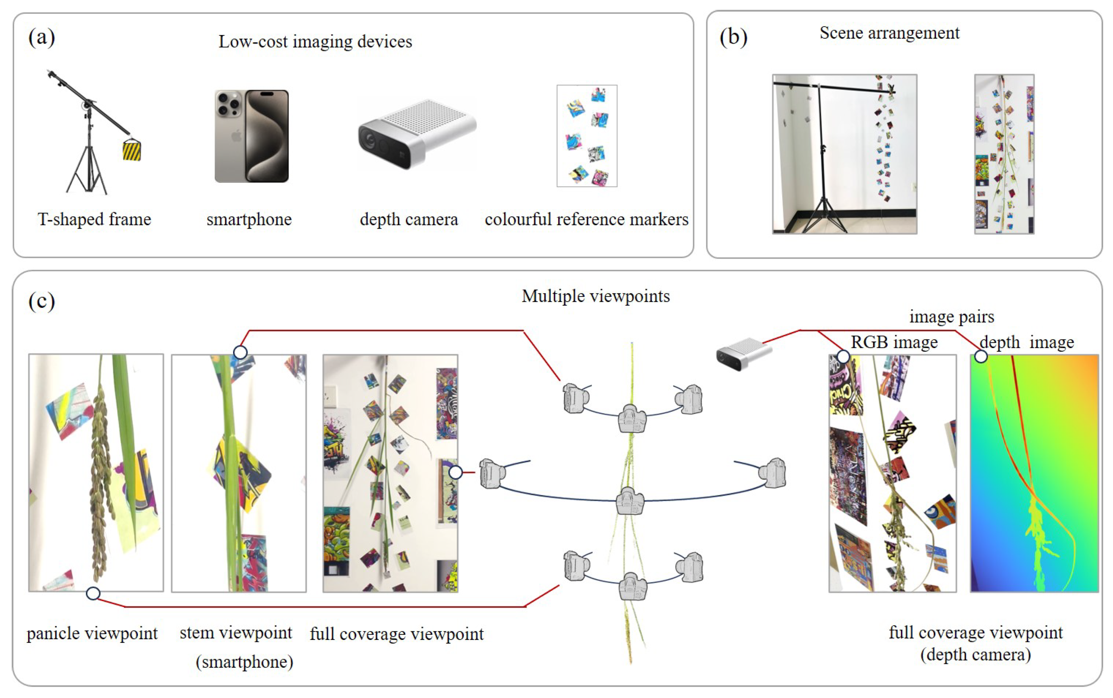
2.2. Reference Markers for Feature Points Matching Enhancement

Because rice tillers were morphologically thin and long relative to other organs, they occupied a relatively small proportion of pixels in the images. In addition, stems and leaves generally lacked distinctive visual features, further complicating robust feature matching during 3D reconstruction. To supply additional feature points for the SfM approach, colorful papers (20 × 20 cm) were attached to the wall as reference markers, thereby enhancing feature-point matching performance. A preliminary experiment showed that these colorful reference markers produced high-quality feature matches, supported stable camera-pose estimation, and ultimately ensured accurate 3D reconstruction. Moreover, even when image pairs exhibited large viewpoint differences, the markers provided accurate and reliable feature correspondence (Figure 2).

2.3. Plant Materials

A panel of 231 japonica rice landraces originating from the Lake Taihu region, located in the Yangtze River Delta near China’s third-largest freshwater lake, was selected for its broad phenotypic diversity. For example, the heading date ranged from 65 to 130 days after sowing, and plant height at heading stage from roughly 80 to 170 cm. The number of productive panicles also differed markedly, spanning 4 to 20 panicles per plant. Panicle architecture encompassed both compact and lax forms, while grain shape ranged from slender to broadly ovate. The diversity of these phenotypes mirrors centuries of farmer selection for yield, local conditions, and varied culinary preferences in the Taihu region.

The plant materials were grown at the experimental farm of Jiangsu Academy of Agricultural Sciences, Nanjing, Jiangsu Province, China (32.0367° N, 118.8802° E) in 2023 (Figure S1). Two rows of each variety were planted with ten plants per row, spaced 17 cm between plants and 20 cm between rows. At the dough stage, tillers were excised, their cut bases were immediately sealed with labeling tape, and the samples were transported to the laboratory within one hour for 3D reconstruction under controlled conditions, thereby preserving native tiller morphology as faithfully as possible. To ensure that each 3D model represented its landrace, preliminary estimations of stem length, leaf length, and panicle height were conducted for each variety, and the tiller whose estimated morphology most closely approximated the landrace average was selected.

2.4. Multi-View Image Capturing

To perform 3D reconstruction of tillers, a simple and low-cost imaging setup was employed that comprised a T-shaped frame, a smartphone (iPhone 15), a depth camera (Microsoft Azure Kinect, Microsoft (China) Co., Ltd., Beijing, China), and colorful reference markers (Figure 3a).

The T-shaped frame was used to suspend and stabilize the tillers. The iPhone 15 (Apple Inc., Cupertino, CA, USA) was chosen for image acquisition because of its high-resolution RGB camera (48 MP, 26 mm focal length, ƒ/1.6 aperture) and advanced image processing capabilities (motion mode, up to 2.8K resolution at 60 fps), which ensured the capture of high-quality, well-focused images even during dynamic image acquisition. The Azure Kinect depth camera was equipped with a 1-megapixel depth sensor capable of capturing paired RGB and depth images, rendering it suitable for consumer-grade applications (Table S1).

Modeling slender objects such as a single rice tiller in 3D was surprisingly challenging. To achieve high-resolution 3D models of a rice tiller, images of each segment in close view were necessary. However, when the lens of the camera was close to a segment of the tiller, the feature points in the images could not be accurately matched for camera pose estimation, since stems and leaves lacked distinct image features and comprised more than 70% of the tiller’s length. As a result, close-view images could not be registered in the coordinate system calculated by SfM. To solve this problem, a different multi-view image-capturing strategy was adopted (Figure 3b). First, the root of a tiller was fixed to a supporting pole using a clamp, and the panicle was hung upside down, as a single tiller could not stand upright naturally. The tiller was then imaged near a wall with colorful reference markers as the background. These reference markers provided feature points to ensure the accuracy of camera pose estimation.

Images from multiple viewpoints were captured by a smartphone and a depth camera (Figure 3c). The smartphone was used to capture RGB images in a 180-degree view around a tiller. At least one depth image was captured by the depth camera for physical scale recovery. Viewpoints were selected to cover various perspectives of the tiller structure. For panicles, the camera was positioned as close as possible to enhance the details. The stem images were taken with careful control of the smartphone’s movement speed to ensure proper image focus. Both RGB and depth cameras were required to capture the entire tiller as a full coverage viewpoint, improving overall image sequence matching.

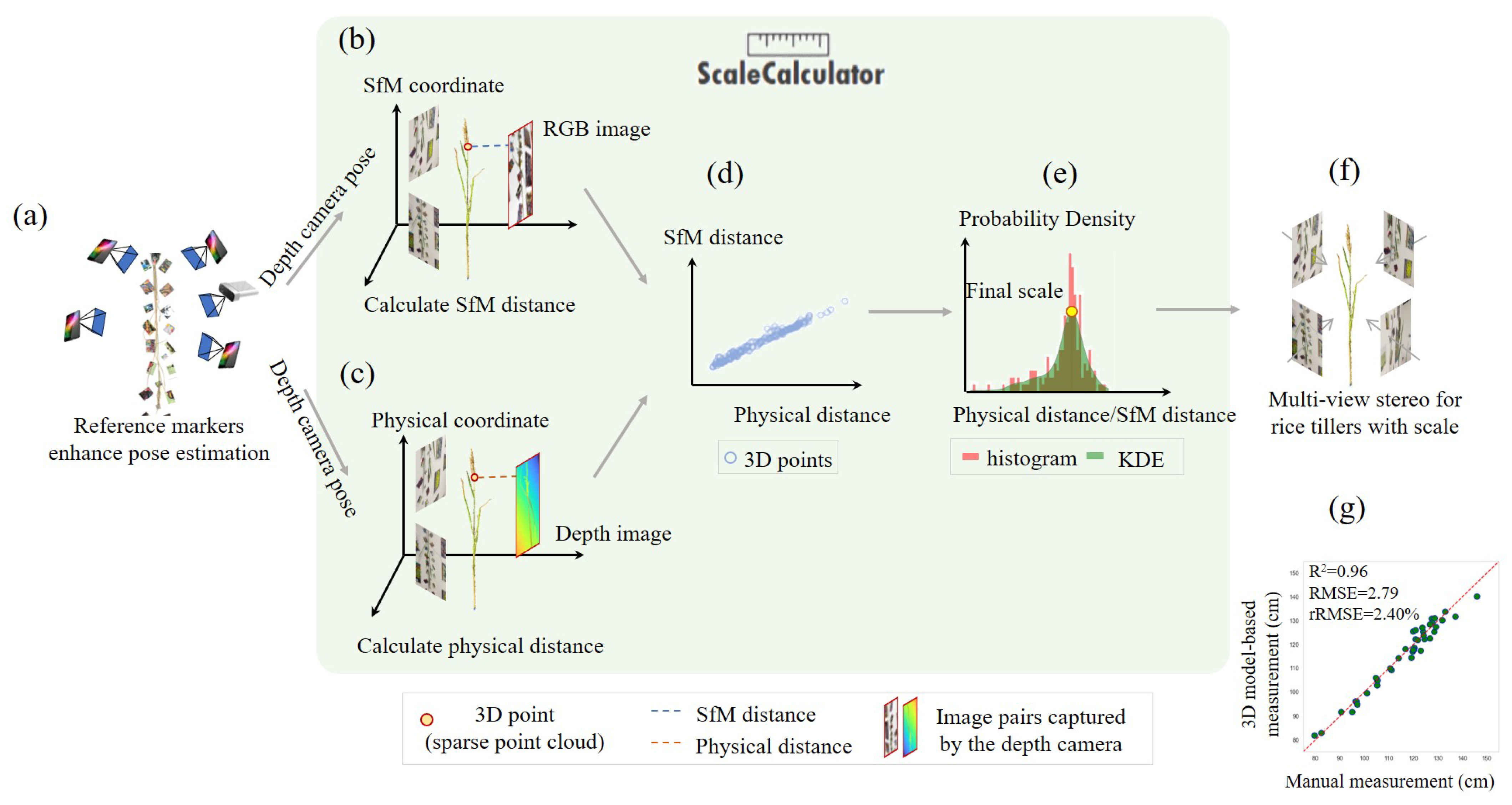
2.5. Recovering the Physical Scale for 3D Models

OSTRA [28] was used to perform pose-estimation and multi-view stereo (MVS) tasks. OSTRA is an open source framework designed for 3D target reconstruction and multilevel segmentation, ensuring the generation of high-quality 3D models. As the models created by OSTRA did not contain the information of the physical size, a custom scale recovery tool, ScaleCalculator, was developed to enable actual-size phenotyping (Figure 4).

At least one depth image captured by a consumer-grade depth camera was required, with each pixel corresponding to the physical distance between the image plane and the object. ScaleCalculator was used to match feature points between the depth image and the corresponding RGB images on the basis of the sparse point cloud generated by SfM. For each matched pair, the relative distances in the SfM coordinate system and the absolute physical distances from the depth sensor were computed and compared, thereby positioning the depth camera within the SfM coordinate system. The SfM coordinate system was adopted because it operated at a relative scale, which avoided the ambiguity that could arise when the world coordinate system, commonly used in computer vision, was employed. The following paragraphs present the derivation of the formula for ScaleCalculator.

Specifically, the RGB images captured by the depth camera and the video frames captured by the smartphone were supplied to the SfM algorithm (Figure 4a). SfM estimated the intrinsic parameters ($f_x$, $f_y$, $c_x$, and $c_y$, where $f_x$ and $f_y$ were the focal lengths and $c_x$ and $c_y$ were the principal points) and the extrinsic parameters ($q_w$, $q_x$, $q_y$, $q_z$, $t_x$, $t_y$, and $t_z$, where $q_w$, $q_x$, $q_y$, and $q_z$ represented camera rotation quaternions in the SfM coordinate system, and $t_x$, $t_y$, and $t_z$ denoted the coordinates of the camera center in the same coordinate system).

In the above setting, the rotation matrix R can be obtained as follows:

$$R=\left[\begin{array}{ccc}1-2q_y^2-2q_z^2& 2q_x{q}_y-2q_z{q}_w& 2q_x{q}_z+2q_y{q}_w\\ 2q_x{q}_y+2q_z{q}_w& 1-2q_x^2-2q_z^2& 2q_y{q}_z-2q_x{q}_w\\ 2q_x{q}_z-2q_y{q}_w& 2q_y{q}_z+2q_x{q}_w& 1-2q_x^2-2q_y^2\end{array}\right]$$

(1)

Let a point $P_w$ in the SfM coordinate system be expressed as follows:

$$P_w=\left[\begin{array}{c}{X}_w\\ Y_w\\ Z_w\end{array}\right]$$

(2)

Assume that the translation vector of the camera in the SfM coordinate system is as follows:

$$t=\left[\begin{array}{c}{t}_x\\ t_y\\ t_z\end{array}\right]$$

(3)

The transformation from SfM coordinates to camera coordinates is as follows:

$$P_c=R{P}_w+t$$

(4)

Substituting (2) and (3) into (4) yields:

$$P_c=R\left[\begin{array}{c}{X}_w\\ Y_w\\ Z_w\end{array}\right]+\left[\begin{array}{c}{t}_x\\ t_y\\ t_z\end{array}\right]$$

(5)

Assuming that $P_c=(X_c,Y_c,Z_c)$, where $Z_c$ is the distance from point $P_w$ to the horizontal plane of the sensor (i.e., the depth of the camera in the SfM coordinate system) (Figure 4b), the following equation is obtained:

$$s_i=\left|Z_c\right|=\left|(2q_x{q}_z-2q_y{q}_w)X_w+(2q_y{q}_z+2q_x{q}_w)Y_w+\left(1-2q_x^2-2q_y^2\right)Z_w+t_z\right|$$

(6)

The depth value of a depth image is defined as the vertical distance from an object to the sensor’s horizontal plane [29]. Each unit of the Azure Kinect’s depth value corresponds to 1 mm in real-world measurements [30]. Therefore, let the physical distance between point i and the horizontal plane of the sensor be $d_i$ (Figure 4c). The ratio between the distance of point i to the horizontal plane of the sensor measured in the SfM coordinate system $s_i$ and the physical distance $d_i$ (Figure 4d), is as follows:

$$k_i={\displaystyle \frac{s_i}{d_i}},i=1,2,\dots ,n$$

(7)

In theory, all of the $k_i$ values are identical. However, in practice, the $k_i$ values follow a normal distribution due to measurement errors. To estimate final scales for corresponding to actual-size 3D models, the optimal bandwidth h was determined via cross-validation, and kernel density estimation (KDE) with a Gaussian kernel was then applied to the set of $k_i$ values.

$$f_h\left(k\right)={\displaystyle \frac{1}{nh}}\sum _{i=1}^{n}K\left(\frac{k-k_i}{h}\right)$$

(8)

where $f_h\left(k\right)$ is the kernel density estimate at point k, K is a kernel function commonly chosen as Gaussian, and h is the window bandwidth. The peak of the Gaussian distribution was defined as the optimum estimate, representing the final scale for converting relative SfM distances into absolute physical measurements (Figure 4e). ScaleCalculator (implemented in Python 3.9) was released as fully open source software, enabling reproduction of the analysis with the processed example data by cloning the repository and running the ScaleCalculator script (Figure S2).

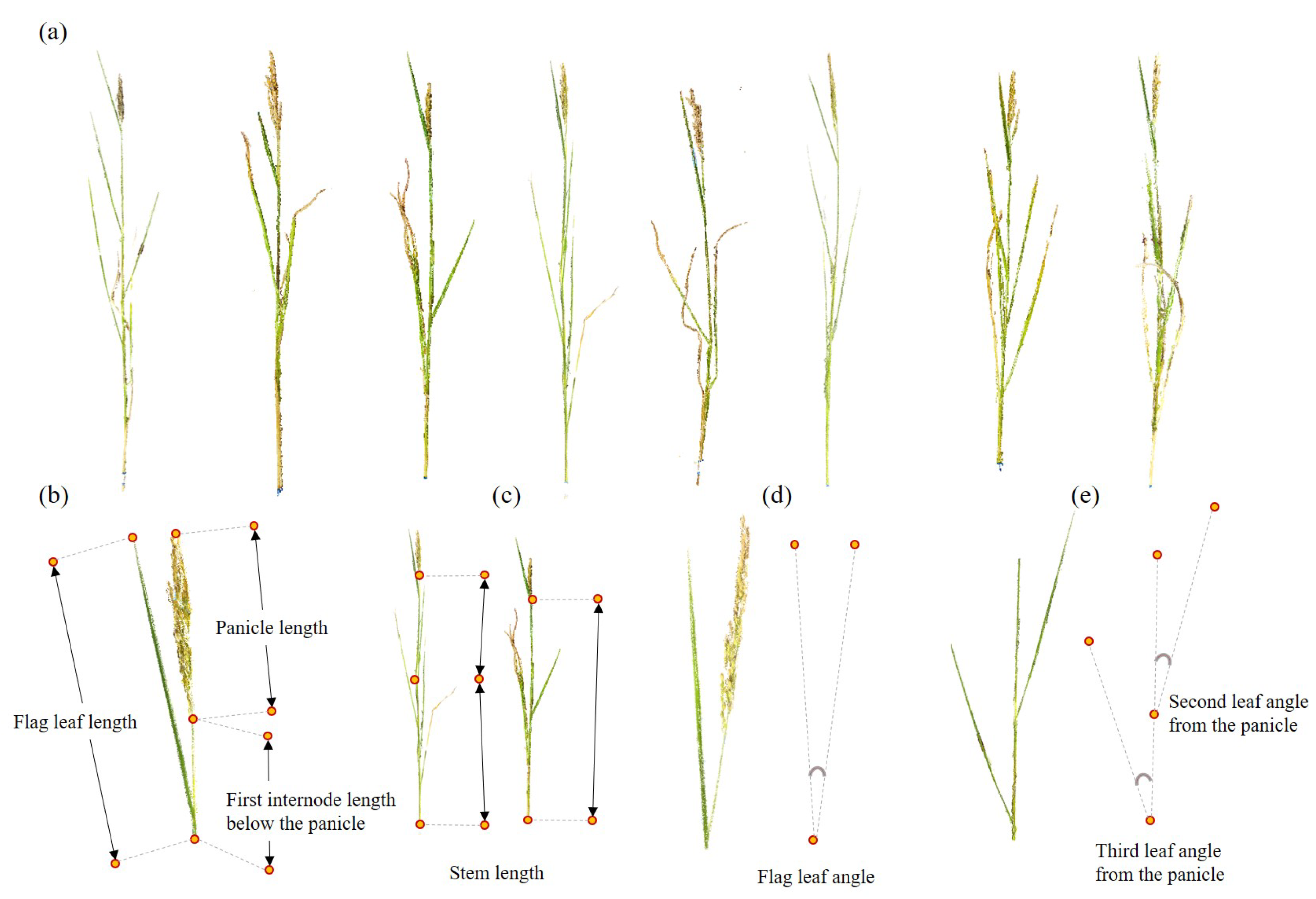
2.6. Three-Dimensional Model-Based Phenotypic Trait Extraction

CloudCompare [31] was employed to carry out morphological analyses of the 3D tiller models and to extract key traits, including panicle length, flag leaf length, first internode length below the panicle, stem length, flag leaf angle, and the angles of the second and third leaves from the panicle (Figure S3). CloudCompare’s point-picking function was used to measure both straight-line distances between point pairs and angles defined by three points. When a stem was bent, its length was measured in segments, and the total length was obtained by summing those segments.

2.7. Genome-Wide Association Study

Three-dimensional rice tiller phenotypic traits were used for subsequent genome-wide association analysis. SNP loci data of 231 rice landraces were obtained from the Institute of Germplasm Resources and Biotechnology, Jiangsu Academy of Agricultural Sciences (unpublished data). The SNP dataset used here corresponds to the same Taihu region japonica rice population analyzed in Zheng et al. [32]. A total of 165,004 SNPs with a minor allele frequency (MAF) > 0.05 were used for GWAS. GWAS was conducted with GEMMA, version 0.98.5 [33], to identify genetic loci associated with tiller morphological traits. GEMMA employed the linear mixed model (LMM) for association, with a kinship matrix to avoid confounding effects [34]. The LMM framework was chosen because its joint modeling of population structure and kinship effectively reduced potential false positives in GWAS results [35]. The model equation is as follows:

$$Y=X\beta +K\mu +ϵ$$

(9)

where Y is the phenotypic value vector, X is the genotype matrix, and $\beta$ is the genotype effect vector. K represents the kinship matrix, while $\mu$ is the random effect vector associated with genetic relatedness. The $ϵ$ denotes the error term. Parameters were estimated using restricted maximum likelihood (REML) estimation. To determine the significance threshold, the Bonferroni method was applied with $P=0.01/n$, where n is the number of effective SNPs. To avoid overcorrection, the significance threshold, $-{log}_{10}\left(P\right)$, in this paper was set to 5.

To monitor residual stratification, the genomic-control inflation factor (${\lambda }_{\mathrm{GC}}$) was computed for each phenotype as follows:

$${\lambda }_{\mathrm{GC}}={\displaystyle \frac{\mathrm{median}\left({\chi }_{\mathrm{obs}}^2\right)}{0.456}}$$

(10)

where $0.456$ is the median of the ${\chi }_1^2$ null distribution. Contemporary large-cohort GWAS regards values between 0.95 and 1.05 [36] as indicating well-calibrated test statistics with negligible confounding, which is an interval adopted.

The LD decay distance of the natural variant population of rice was approximately 200 kb [37]. Because the Taihu landrace panel analyzed here was identical to that used in earlier GWAS investigations of the region’s germplasm [32], a 200 kb window on either side of each lead SNP was adopted when defining association intervals. Raw phenotypic traits were filtered according to two criteria. First, measurements for certain tillers were discarded when partial dryness or defects rendered them inaccurate. Second, statistical outliers were excluded to promote a normal distribution of the data. After these filtering steps, the cleaned phenotypic data were used to conduct the GWAS, ensuring that the reported results can be reproduced in conjunction with the accompanying genotype data.

3. Results

3.1. High-Resolution 3D Rice Tiller Models

High-resolution 3D tiller models for 231 rice landraces were reconstructed with reference markers that enhanced feature-point detection (Figure 5a). Each 3D model was reconstructed using around 300 RGB images, complemented by one depth image to recover the physical scale. The final 3D tiller models for 231 landraces created in this study are available online. The accuracy of the 3D tiller models was assessed by comparing model-based tiller-length measurements with manual measurements, using the following three evaluation metrics: the coefficient of determination (R²), root mean square error (RMSE), and relative root mean square error (rRMSE). Tiller length from the base of the stem to the panicle was selected as the primary validation metric because it represents a fundamental structural trait that spans the entire tiller architecture. Furthermore, unlike angle measurements are susceptible to subjective operational errors, tiller length is straightforward for precise measurements from the base to the panicle. It makes tiller length an ideal metric for evaluating the accuracy of scale calibration in the reconstructed 3D models. A total of 40 models were randomly selected for tiller length analysis. The x-axis represents the physical measurements, while the y-axis corresponds to the values obtained directly from the 3D plant models. Experimental results demonstrated a strong linear correlation (R² = 0.96), with RMSE and rRMSE values of 2.79 cm and 2.40%, respectively (Figure 4g). These results validate the accuracy of the 3D model’s structure and the effectiveness of the ScaleCalculator in recovering the physical scale.

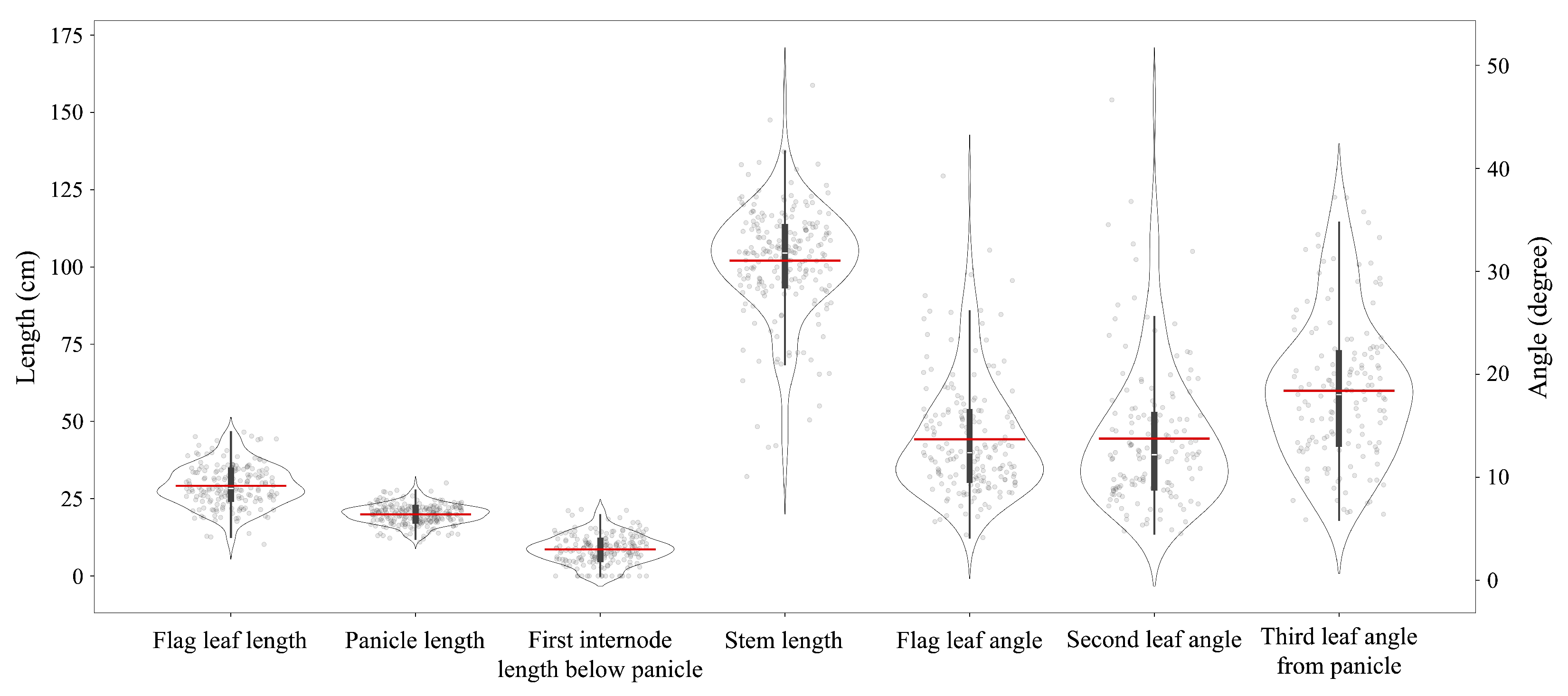
3.2. Phenotypic Traits by 3D Rice Tiller Models

High-resolution 3D tiller models enabled the development of mathematical or computer vision methods for extracting phenotypic traits that are difficult to measure manually. As a proof of concept, seven agronomic traits were extracted from the 3D tiller models of 231 rice landraces, including flag leaf length, panicle length, first internode length below the panicle, stem length, flag leaf angle, second leaf angle from the panicle and third leaf angle from the panicle (Figure 5b and Figure S3). The Supplementary Materials (Table S2) provide the cleaned phenotypic dataset derived from the 3D models for these 231 tillers. Descriptive analysis of the traits revealed considerable variation among the landraces (Figure 6 and Table S3).

The measurements revealed substantial diversity across the key phenotypic traits. For instance, flag leaf length ranged from 10.24 to 46.55 cm (mean = 29.18 cm), and panicle length varied from 10.97 to 30.11 cm (mean = 19.93 cm). In addition, the standard deviation (SD) values further emphasize this variability. For example, an SD of 6.79 for flag leaf length indicates that individual measurements typically deviate by nearly 7 cm from the mean, highlighting the broad dispersion of flag leaf sizes. In contrast, an SD of 3.18 for panicle length suggests relatively more consistency in this trait. Unlike the cultivated varieties selected for the agricultural industry, the landraces preserved distinct morphological structures and phenotypic traits, as revealed by the actual-size 3D models.

A correlation analysis was performed on seven rice phenotypic traits. The results revealed a moderate positive correlation (r = 0.46) between flag leaf length and panicle length, suggesting that, as the primary photosynthetic organ, a longer flag leaf may promote panicle development and ultimately increase yield, which is in agreement with previous studies. Additionally, the internode immediately below the panicle exhibited a moderate positive correlation with the second leaf angle from the panicle (r = 0.42), whereas stem length was negatively correlated with the second leaf angle from the panicle (r = −0.38). Overall, the low-to-moderate correlation coefficients are consistent with the complex genetic and environmental regulation of rice phenotypic traits (Figure S4).

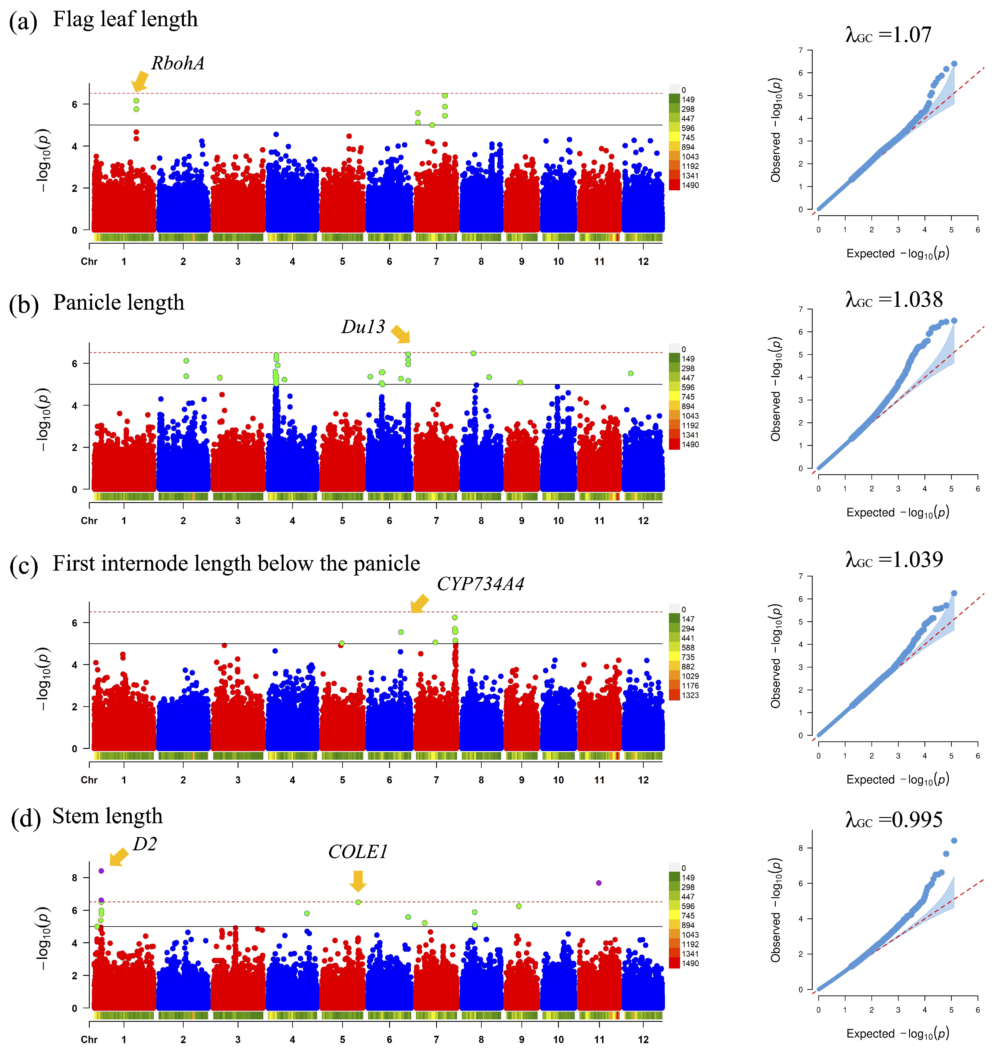
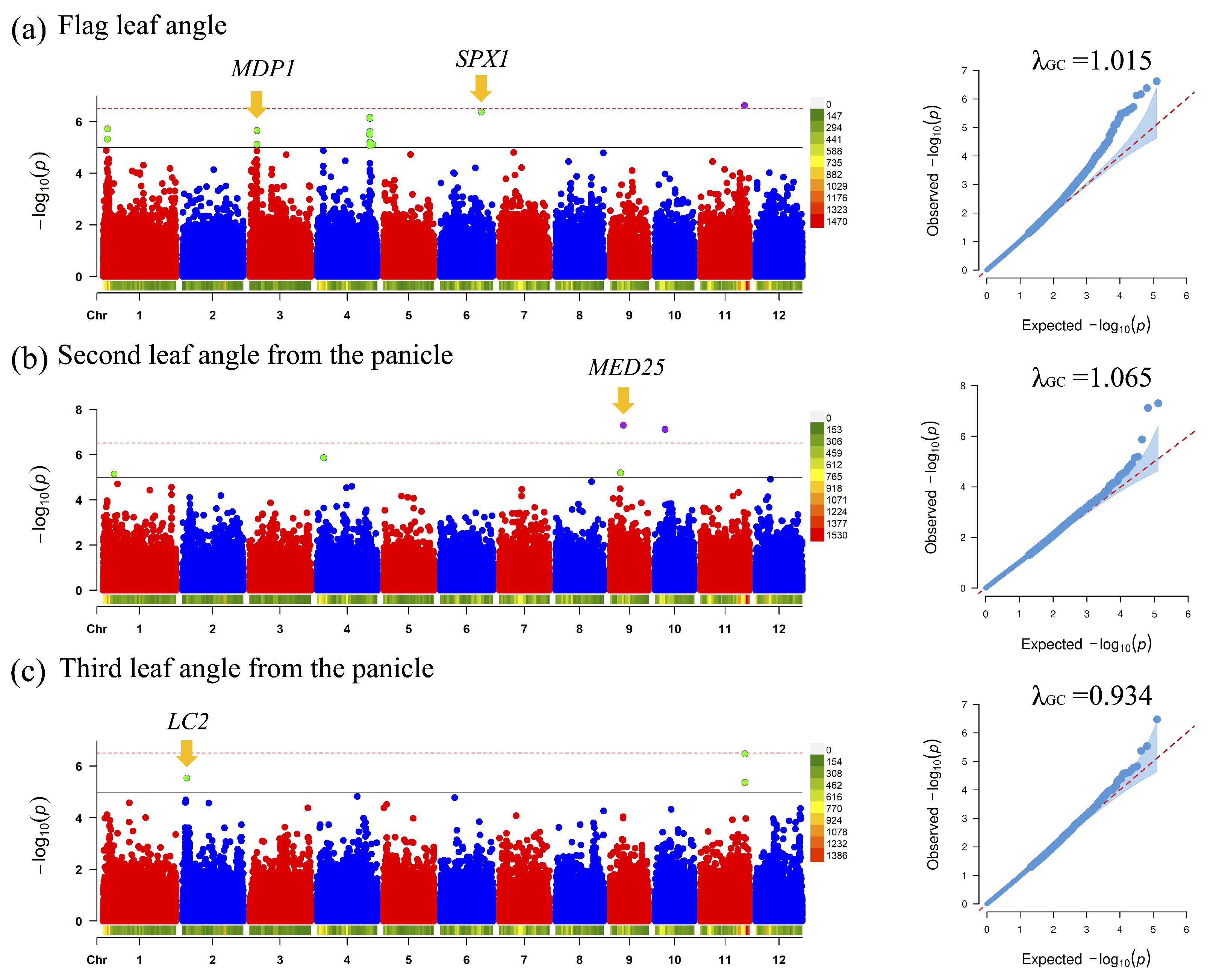
3.3. GWAS for 3D Rice Tiller Phenotypes

To demonstrate the effectiveness and utilization of the 3D model approach in genetic studies for poorly structured agricultural objects such as rice tillers, genome-wide association studies (GWAS) were conducted (Figure 7 and Figure 8). In this study, 165,004 SNPs with MAF > 5% were obtained internally as genetic variance data to investigate the underlying genetic basis of seven phenotypic traits measured from 3D rice tiller models of 231 rice landraces. A total of 93 (SNPs passing the p-value threshold) significant SNPs were identified by GWAS. Nine lead SNPs at loci associated with the seven traits were identified, and candidate genes at these loci were mapped. Previously reported rice tiller related genes that may influence agronomic traits under diverse environmental conditions were also pinpointed (Table S4).

First, at Chr3:30,585,253, a lead SNP associated with flag leaf length was identified (Figure 7a). This SNP was located near RbohA, which regulated the production of reactive oxygen species (ROS), affecting signaling pathways under water stress and thus controlling flag leaf growth and development in rice [38]. Moreover, a lead SNP at Chr6:29,179,707 associated with panicle length was identified (Figure 7b). This variant was located upstream of Du13, which regulated panicle growth by modulating the expression of genes involved in grain development, thereby affecting overall panicle length in rice [39]. Similarly, for the first internode length below the panicle, a lead SNP at Chr6:23,847,193 was uncovered that lay downstream of CYP734A4 (Figure 7c), which mediated the degradation of plant steroid hormones and thus regulated the development of the first internode below the panicle [40]. In the GWAS for stem length, two notable lead SNPs were detected. D2 was located around the SNP at Chr1:5,005,598, (Figure 7d), which positively regulated the longitudinal elongation of stem cells by modulating brassinosteroid biosynthesis, thereby influencing internode length and overall plant height [41]. COLE1 was situated near the other SNP at Chr5:26,469,145 (Figure 7d), which modulated the level of free indole-3-acetic acid (IAA) at the base of the stem, ultimately affecting cell size and stem length [42].

Furthermore, in the GWAS for flag leaf angle, two lead SNPs and candidate genes were identified. MDP1 near one SNP at Chr3:4,397,619 (Figure 8a) was a MADS-box transcription factor that was expressed in the matured leaf and negatively regulates genes associated with cell expansion, particularly under light-induced or brassinosteroid conditions, thereby shaping the leaf angle [43]. SPX1 around the other SNP at Chr6:24,296,365 (Figure 8a) interacted with RLI1 to repress its transcriptional activity, thereby negatively regulating the flag leaf angle [44]. For the second leaf angle from the panicle, a lead SNP at Chr9:7,822,293 was identified upstream of MED25 (Figure 8b), which modulated the leaf angle by influencing plant hormone signaling and transcription factor activity [45]. For the third leaf angle from the panicle, a SNP identified at Chr2:2,541,557 lies upstream of LC2 (Figure 8c), a gene that inhibits epidermal cell division in the leaf sheath tip, thereby determining leaf angle size [46].

To assess whether the GWAS results were inflated by residual population stratification or cryptic relatedness, the genomic-control inflation factor (${\lambda }_{\mathrm{GC}}$) was calculated for each trait (Figure 7 and Figure 8). Across the seven phenotypes, ${\lambda }_{\mathrm{GC}}$ ranged from 0.934 to 1.070. Five traits exhibited values very close to the null expectation of 1 (flag leaf angle = 1.015; panicle length = 1.038; first internode length = 1.039; stem length = 0.995; third leaf angle = 0.934). Only second leaf angle from the panicle (${\lambda }_{\mathrm{GC}}=1.065$) and flag leaf length (${\lambda }_{\mathrm{GC}}=1.070$) exceeded the commonly used cautionary threshold of 1.05, indicating mild but non-negligible genomic inflation for these traits. The near-unity values observed for the remaining phenotypes indicate that the linear mixed model (LMM) incorporating a kinship matrix has effectively controlled for confounding effects.

4. Discussion

4.1. Three-Dimensional Models for Rice Production

The distinct morphological features of rice tiller play a vital role in shaping overall plant architecture and influencing yield. As such, isolating and reconstructing a single tiller model allows for a more targeted and detailed analysis of key traits, including leaf angle, stem length, and panicle structure. The GWAS on 231 rice landraces identified nine previously reported genes associated with tiller architecture. Among them, RbohA is known for its vital roles in flag leaf growth between the wild type and RbohA mutant rice plants by regulating ROS production and influencing key signaling pathways in rice development and drought responses [38]. Another well-studied gene, LC2, was reported with its function to govern leaf angle by inhibiting epidermal cell proliferation at the leaf sheath tip, thereby determining the final leaf angle [46]. Additionally, D2, which regulates stem length by modulating brassinosteroid biosynthesis, positively controls the longitudinal elongation of cells in the rice stem, ultimately affecting internode length and overall stem height [41]. To summarize, these findings align with prior functional studies, validating the biological relevance of phenotypic traits extracted from the 3D models of rice tillers.

These findings underscore the potential of 3D modeling for applications in rice production and breeding programs. Over the next decade, rice yield is projected to increase by approximately 12%, while overall rice production is expected to grow by 2.4% [47]. These gains will largely be driven by the intensification of production on limited arable land, supported by advances in agricultural technology and improved cultivation practices. Within this context, the proposed low-cost 3D phenotyping pipeline could be integrated into routine breeding workflows as a rapid decision support tool. By providing millimeter-scale digital measurements of key traits such as stem length, internode spacing, and leaf angle, the pipeline enables breeders to more precisely identify landraces or breeding lines that align with target plant architectures. Moreover, because the imaging system requires only a smartphone and a consumer-grade depth sensor, it can be readily deployed in frontline breeding nurseries, thereby reducing technical and financial barriers for small and medium scale breeding programs.

4.2. Applicability to Other Species

The approach introduced in this study can be easily transferred to other crop species with slender organs and low self-occlusion. For example, researchers can adapt the approach to major cereal crops such as wheat, barley, rye, and oat to measure the lengths and angles of their thin and long stems, internodes, or leaves. Moreover, the method can be applied to crops that have been explored with 2D imaging but are still in the initial stages of 3D phenotyping, such as sorghum and pearl millet for measuring panicle size. Beyond cereals, the same principles extend to other monocots that produce elongated floral or vegetative structures (e.g., sugarcane internodes, Brachypodium tillers or even lily scapes), while the hurdle of technique transfer of this method is expected to be low with simple and portable experimental setup and devices of a small budget, there are three practical considerations as follows: organ size, viewpoint coverage, and camera working distance. Specifically, larger organs (e.g., mature sugarcane sections) demand a wider field of view, and an operator therefore has to increase the stand-off distance while ensuring that the organ remains within the depth sensor’s optimal range. Likewise, to prevent missing data at the distal ends of very long organs, the number of acquisition angles should be increased to maintain homogeneous point density along the entire length. Thus, the workflow can be applied directly to most slender cereal organs with modest adjustments to imaging geometry by breeders as a practical tool to quantify subtle architectural traits at a population scale.

4.3. Challenges and Future Directions

Despite these promising results, there are still challenges that need to be addressed. First, the tillers were reconstructed in an inverted orientation to prevent structural bending artifacts caused by their slender morphology and the weight of panicles in their natural upright position. Since the formation of rice leaf angles is primarily regulated by plant hormones and gravity, the leaf angle measured in this study differs from its traditional definition. Second, phenotypic trait data from 3D models contained incomplete or missing values due to wilting and physical damage sustained by rice tillers during transport from field to laboratory for imaging. In future studies, because the landraces in the panel span a wide range of heading dates (65–132 days after sowing), it is recommended to ensure that the number of experimental objects remains within a manageable level each day. Additionally, setting up a simple imaging station with a canopy and backdrop at the edge of the plot will help us photograph each tiller right after cutting. This procedure will minimize dehydration-induced wilting and preserve delicate phenotypes such as leaf angle. In parallel, in situ imaging platforms are being actively explored to enable future investigations to be conducted entirely under field conditions, thereby eliminating transfer effects altogether. Third, in this study, manual measurement focused only on tiller length, and other phenotypic traits were not validated through correlation analysis. To address this, a sufficient number of dedicated technicians will be assigned in future experiments. This arrangement will facilitate comprehensive validation of every reported trait, especially angles and internode lengths, and, by shortening the interval between image capture and manual measurement, it will reduce errors introduced by delayed measurements. Lastly, although the current method produces high-resolution models, the data acquisition process still requires manual intervention for tiller fixation, viewpoint adjustment, and image capture, taking an average of five minutes of manual work per tiller. It limits throughput, especially for large datasets, and it may hinder large-scale population studies. To improve the reconstruction efficiency, future work should focus on robotic solutions for automated data collection. For example, employing robotic arms for viewpoint navigation or developing robotic platforms with synchronized RGBD sensors could significantly increase throughput.

5. Conclusions

This study developed a method for reconstructing rice tiller 3D models for genetic research by generating accurate and reproducible morphological traits from the models. Low-cost, readily available equipment captured high-resolution images from multiple viewpoints for 3D reconstruction, while strategically placed colorful reference markers supplied robust feature points to mitigate the challenges posed by slender tiller morphology. Depth images were incorporated to restore actual scale automatically through a custom tool, ScaleCalculator. Correlation analysis between manual measurements and 3D-model-derived tiller lengths demonstrated high accuracy and robustness, indicating that the workflow can be adapted to other crops with comparable morphological constraints. Genome-wide association studies based on these 3D phenotypes validated the biological relevance of the approach by recovering several genes previously implicated in rice tiller development. Overall, the work provides a reproducible and scalable platform for dissecting the genetic basis of complex plant morphologies, with the potential to accelerate understanding of plant organ architecture and to support the more precise selection of desirable traits in crop breeding.

References

1. Food and Agriculture Organization of the United Nations (FAO). FAOSTAT: Production Quantity (Crops). Available online: https://www.fao.org/faostat/en/#data/QCL (accessed on 5 July 2025).
2. Yuan, R.; Mao, Y.; Zhang, D.; Wang, S.; Zhang, H.; Wu, M.; Ye, M.; Zhang, Z. The formation of rice tillers and factors influencing it. Agronomy 2024, 14, 2904. [Google Scholar] [CrossRef]
3. Huang, M.; Shan, S.; Cao, J.; Fang, S.; Tian, A.; Liu, Y.; Cao, F.; Yin, X.; Zou, Y. Primary-tiller panicle number is critical to achieving high grain yields in machine-transplanted hybrid rice. Sci. Rep. 2020, 10, 2811. [Google Scholar] [CrossRef]
4. Tsugawa, S.; Shima, H.; Ishimoto, Y.; Ishikawa, K. Thickness-stiffness trade-off improves lodging resistance in rice. Sci. Rep. 2023, 13, 10828. [Google Scholar] [CrossRef]
5. Wu, D.; Guo, Z.; Ye, J.; Feng, H.; Liu, J.; Chen, G.; Zheng, J.; Yan, D.; Yang, X.; Xiong, X.; et al. Combining high-throughput micro-CT-RGB phenotyping and genome-wide association study to dissect the genetic architecture of tiller growth in rice. J. Exp. Bot. 2019, 70, 545–561. [Google Scholar] [CrossRef] [PubMed]
6. Huang, Y.; Xia, P.; Gong, L.; Chen, B.; Li, Y.; Liu, C. Designing an interactively cognitive humanoid field-phenotyping robot for in-field rice tiller counting. Agriculture 2022, 12, 1966. [Google Scholar] [CrossRef]
7. Van Crombrugge, I.; Sels, S.; Ribbens, B.; Steenackers, G.; Penne, R.; Vanlanduit, S. Accuracy assessment of joint angles estimated from 2D and 3D camera measurements. Sensors 2022, 22, 1729. [Google Scholar] [CrossRef] [PubMed]
8. Ayaz, I.; Shaheen, E.; Aly, M.; Shujaat, S.; Gallo, G.; Coucke, W.; Politis, C.; Jacobs, R. Accuracy and reliability of 2-dimensional photography versus 3-dimensional soft tissue imaging. Imaging Sci. Dent. 2020, 50, 15–22. [Google Scholar] [CrossRef]
9. Kenchanmane Raju, S.K.; Adkins, M.; Enersen, A.; Santana de Carvalho, D.; Studer, A.J.; Ganapathysubramanian, B.; Schnable, P.S.; Schnable, J.C. Leaf Angle eXtractor: A high-throughput image processing framework for leaf angle measurements in maize and sorghum. Appl. Plant Sci. 2020, 8, e11385. [Google Scholar] [CrossRef]
10. Tross, M.C.; Gaillard, M.; Zwiener, M.; Miao, C.; Grove, R.J.; Li, B.; Benes, B.; Schnable, J.C. 3D reconstruction identifies loci linked to variation in angle of individual sorghum leaves. PeerJ 2021, 9, e12628. [Google Scholar] [CrossRef]
11. Xu, J. GrainShape: A landmark-annotated image dataset of japonica rice grains for geometric morphometric analysis. Data Brief 2025, 61, 111781. [Google Scholar] [CrossRef]
12. Paturkar, A.; Sen Gupta, G.; Bailey, D. Making use of 3D models for plant physiognomic analysis: A review. Remote Sens. 2021, 13, 2232. [Google Scholar] [CrossRef]
13. Wang, K.; Pu, X.; Li, B. Automated phenotypic trait extraction for rice plant using terrestrial laser scanning data. Sensors 2024, 24, 4322. [Google Scholar] [CrossRef]
14. Pound, M.P.; French, A.P.; Fozard, J.A.; Murchie, E.H.; Pridmore, T.P. A patch-based approach to 3D plant shoot phenotyping. Mach. Vis. Appl. 2016, 27, 767–779. [Google Scholar] [CrossRef]
15. Schonberger, J.L.; Frahm, J.M. Structure-from-motion revisited. In Proceedings of the IEEE Conference on Computer Vision and Pattern Recognition, Las Vegas, NV, USA, 27–30 June 2016; pp. 4104–4113. [Google Scholar]
16. Schönberger, J.L.; Zheng, E.; Frahm, J.M.; Pollefeys, M. Pixelwise view selection for unstructured multi-view stereo. In Proceedings of the Computer Vision-ECCV 2016: 14th European Conference, Amsterdam, The Netherlands, 11–14 October 2016; pp. 501–518. [Google Scholar]
17. Cernea, D. OpenMVS: Multi-View Stereo Reconstruction Library. Available online: https://github.com/cdcseacave/openMVS (accessed on 28 December 2024).
18. Sandhu, J.; Zhu, F.; Paul, P.; Gao, T.; Dhatt, B.K.; Ge, Y.; Staswick, P.; Yu, H.; Walia, H. PI-Plat: A high-resolution image-based 3D reconstruction method to estimate growth dynamics of rice inflorescence traits. Plant Methods 2019, 15, 162. [Google Scholar] [CrossRef]
19. Dharni, J.S.; Dhatt, B.K.; Paul, P.; Gao, T.; Awada, T.; Bacher, H.; Peleg, Z.; Staswick, P.; Hupp, J.; Yu, H.; et al. A non-destructive approach for measuring rice panicle-level photosynthetic responses using 3D-image reconstruction. Plant Methods 2022, 18, 126. [Google Scholar] [CrossRef] [PubMed]
20. Mildenhall, B.; Srinivasan, P.P.; Tancik, M.; Barron, J.T.; Ramamoorthi, R.; Ng, R. NeRF: Representing scenes as neural radiance fields for view synthesis. In Lecture Notes in Computer Science; Springer International Publishing: Cham, Switzerland, 2020; pp. 405–421. [Google Scholar]
21. Yang, X.; Lu, X.; Xie, P.; Guo, Z.; Fang, H.; Fu, H.; Hu, X.; Sun, Z.; Cen, H. PanicleNeRF: Low-cost, high-precision in-field phenotyping of rice panicles with smartphone. Plant Phenomics 2024, 6, 0279. [Google Scholar] [CrossRef] [PubMed]
22. Gong, L.; Du, X.; Zhu, K.; Lin, K.; Lou, Q.; Yuan, Z.; Huang, G.; Liu, C. Panicle-3D: Efficient phenotyping tool for precise semantic segmentation of rice Panicle point cloud. Plant Phenomics 2021, 2021, 9838929. [Google Scholar] [CrossRef]
23. Cui, D.; Liu, P.; Liu, Y.; Zhao, Z.; Feng, J. Automated Phenotypic Analysis of Mature Soybean Using Multi-View Stereo 3D Reconstruction and Point Cloud Segmentation. Agriculture 2025, 15, 175. [Google Scholar] [CrossRef]
24. Yang, D.; Yang, H.; Liu, D.; Wang, X. Research on Automatic 3D Reconstruction of Plant Phenotype Based on Multi-View Images. Comput. Electron. Agric. 2024, 220, 108866. [Google Scholar] [CrossRef]
25. He, W.; Ye, Z.; Li, M.; Yan, Y.; Lu, W.; Xing, G. Extraction of soybean plant trait parameters based on SfM–MVS algorithm combined with GRNN. Front. Plant Sci. 2023, 14, 1181322. [Google Scholar] [CrossRef]
26. Wu, S.; Wen, W.; Gou, W.; Lu, X.; Zhang, W.; Zheng, C.; Xiang, Z.; Chen, L.; Guo, X. A miniaturized phenotyping platform for individual plants using multi-view stereo 3D reconstruction. Front. Plant Sci. 2022, 13, 897746. [Google Scholar] [CrossRef]
27. Li, S.; Li, J.; Yang, T.; A, X.; Liu, J. Incremental Structure from Motion for Small-Scale Scenes Based on Auxiliary Calibration. Sensors 2025, 25, 415. [Google Scholar] [CrossRef]
28. Xu, J.; Zhao, W.; Tang, Z.; Gan, X. A One Stop 3D Target Reconstruction and multilevel Segmentation Method. arXiv 2023, arXiv:2308.06974. [Google Scholar] [CrossRef]
29. Laina, I.; Rupprecht, C.; Belagiannis, V.; Tombari, F.; Navab, N. Deeper depth prediction with fully convolutional residual networks. In Proceedings of the 2016 4th International Conference on 3D Vision (3DV), Stanford, CA, USA, 25–28 October 2016; pp. 239–248. [Google Scholar]
30. Tölgyessy, M.; Dekan, M.; Chovanec, Ľ.; Hubinský, P. Evaluation of the Azure Kinect and its comparison to Kinect V1 and Kinect V2. Sensors 2021, 21, 413. [Google Scholar] [CrossRef] [PubMed]
31. CloudCompare (Version 2.14.alpha): 3D Point Cloud and Mesh Processing Software. Available online: https://www.danielgm.net/cc/ (accessed on 6 July 2025).
32. Zheng, H.; Tang, W.; Yang, T.; Zhou, M.; Guo, C.; Cheng, T.; Cao, W.; Zhu, Y.; Zhang, Y.; Yao, X. Grain protein content phenotyping in rice via hyperspectral imaging technology and a genome-wide association study. Plant Phenomics 2024, 6, 0200. [Google Scholar] [CrossRef] [PubMed]
33. Zhou, X.; Stephens, M. Genome-wide efficient mixed-model analysis for association studies. Nat. Genet. 2012, 44, 821–824. [Google Scholar] [CrossRef] [PubMed]
34. Uffelmann, E.; Huang, Q.Q.; Munung, N.S.; De Vries, J.; Okada, Y.; Martin, A.R.; Martin, H.C.; Lappalainen, T.; Posthuma, D. Genome-wide association studies. Nat. Rev. Methods Prim. 2021, 1, 59. [Google Scholar] [CrossRef]
35. Alamin, M.; Sultana, M.H.; Lou, X.; Jin, W.; Xu, H. Dissecting Complex Traits Using Omics Data: A Review on the Linear Mixed Models and Their Application in GWAS. Plants 2022, 11, 3277. [Google Scholar] [CrossRef]
36. Castel, S.E.; Tluway, F.D.; Emde, A.K.; Smyth, N.; Karim, M.; Sengupta, D.; Gray, O.A.; Hendershott, M.; LeBaron von Baeyer, S.; Burke, E.E.; et al. A map of blood regulatory variation in South Africans enables GWAS interpretation. Nat. Genet. 2025, 57, 1628–1637. [Google Scholar] [CrossRef]
37. Xu, X.; Ye, J.; Yang, Y.; Zhang, M.; Xu, Q.; Feng, Y.; Yuan, X.; Yu, H.; Wang, Y.; Yang, Y.; et al. Genome-wide association study of rice rooting ability at the seedling stage. Rice 2020, 13, 59. [Google Scholar] [CrossRef]
38. Wang, X.; Zhang, M.M.; Wang, Y.J.; Gao, Y.T.; Li, R.; Wang, G.F.; Li, W.Q.; Liu, W.T.; Chen, K.M. The plasma membrane NADPH oxidase OsRbohA plays a crucial role in developmental regulation and drought-stress response in rice. Physiol. Plant. 2016, 156, 421–443. [Google Scholar] [CrossRef]
39. Cai, Y.; Zhang, W.; Fu, Y.; Shan, Z.; Xu, J.; Wang, P.; Kong, F.; Jin, J.; Yan, H.; Ge, X.; et al. Du13 encodes a C2 H2 zinc-finger protein that regulates Wxb pre-mRNA splicing and microRNA biogenesis in rice endosperm. Plant Biotechnol. J. 2022, 20, 1387–1401. [Google Scholar] [CrossRef]
40. Zhan, C.; Hu, J.; Pang, Q.; Yang, B.; Cheng, Y.; Xu, E.; Zhu, P.; Li, Y.; Zhang, H.; Cheng, J. Genome-wide association analysis of panicle exsertion and uppermost internode in rice (Oryza sativa L.). Rice 2019, 12, 72. [Google Scholar] [CrossRef]
41. Hong, Z.; Ueguchi-Tanaka, M.; Umemura, K.; Uozu, S.; Fujioka, S.; Takatsuto, S.; Yoshida, S.; Ashikari, M.; Kitano, H.; Matsuoka, M. A rice brassinosteroid-deficient mutant, ebisu dwarf (d2), is caused by a loss of function of a new member of cytochrome P450. Plant Cell 2003, 15, 2900–2910. [Google Scholar] [CrossRef] [PubMed]
42. Liu, F.; Zhang, L.; Luo, Y.; Xu, M.; Fan, Y.; Wang, L. Interactions of Oryza sativa Os CONTINUOUS VASCULAR RING-LIKE 1 (Os COLE1) and Os COLE1-INTERACTING PROTEIN reveal a novel intracellular auxin transport mechanism. New Phytol. 2016, 212, 96–107. [Google Scholar] [CrossRef] [PubMed]
43. Duan, K.; Li, L.; Hu, P.; Xu, S.P.; Xu, Z.H.; Xue, H.W. A brassinolide-suppressed rice MADS-box transcription factor, OsMDP1, has a negative regulatory role in BR signaling. Plant J. 2006, 47, 519–531. [Google Scholar] [CrossRef] [PubMed]
44. Ruan, W.; Guo, M.; Xu, L.; Wang, X.; Zhao, H.; Wang, J.; Yi, K. An SPX-RLI1 module regulates leaf inclination in response to phosphate availability in rice. Plant Cell 2018, 30, 853–870. [Google Scholar] [CrossRef]
45. Karkute, S.G.; Kumar, V.; Tasleem, M.; Mishra, D.C.; Chaturvedi, K.K.; Rai, A.; Sevanthi, A.M.; Gaikwad, K.; Sharma, T.R.; Solanke, A.U. Genome-wide analysis of von Willebrand factor A gene family in rice for its role in imparting biotic stress resistance with emphasis on rice blast disease. Rice Sci. 2022, 29, 375–384. [Google Scholar] [CrossRef]
46. Zhao, S.Q.; Hu, J.; Guo, L.B.; Qian, Q.; Xue, H.W. Rice leaf inclination2, a VIN3-like protein, regulates leaf angle through modulating cell division of the collar. Cell Res. 2010, 20, 935–947. [Google Scholar] [CrossRef]
47. Organisation for Economic Co-operation and Development; Food and Agriculture Organization of the United Nations (OECD/FAO). OECD Agriculture Statistics (Database): OECD-FAO Agricultural Outlook 2022–2031. Available online: https://www.oecd.org/en/publications/oecd-fao-agricultural-outlook-2022-2031_f1b0b29c-en.html (accessed on 5 July 2025).
Figure 1. Workflow for 3D tiller model creation and genome-wide association analysis. (a) Multi-view tiller data acquisition was performed using a smartphone and a depth camera. (b) 3D models were reconstructed from RGB images captured from multiple perspectives. Colorful reference markers were used to enhance pose estimation performance. ScaleCalculator was used to estimate parameters for actual-size adjustment by integrating depth image data. The estimated results from ScaleCalculator were then applied to recover the 3D models generated by multi-view stereo (MVS), producing actual-size 3D models. (c) These models were subjected to morphological analysis, including flag leaf length, panicle length, first internode length below the panicle, stem length, flag leaf angle, second leaf angle from the panicle, and third leaf angle from the panicle. (d) Subsequently, genome-wide association analysis was performed on these phenotypic traits.
Agronomy 15 01803 g001
Figure 2. Multi-view image matching. In image matching, reference markers provided a dense set of effective feature points, which facilitated the formation of robust correspondences. In contrast, although rice tillers exhibited numerous feature points, they failed to yield reliable correspondences. (a) The panicle and flag leaf. (b) The stem. (c) The leaf. (d) The whole tiller.
Agronomy 15 01803 g002
Figure 3. Multi-view tiller data acquisition. (a) The imaging devices include a T-shaped frame, a smartphone (iPhone 15 used in this study), a depth camera (Microsoft Azure Kinect used in this study), and colorful reference markers. (b) The T-shaped frame was used to suspend and stabilize the tillers. The colorful reference markers were affixed to a wall, serving as the background for capturing the tillers. The operator utilized the smartphone’s sport mode for optimal results. (c) Viewpoint selection was categorized into the following three types: panicle, stem, and full coverage viewpoints, ensuring detailed reconstruction of the tiller and complete coverage from all angles.
Agronomy 15 01803 g003
Figure 4. Actual-size 3D rice tiller reconstruction. (a) The depth camera and smartphone both participated in pose estimation, with colorful reference markers arranged in the reconstruction scene to enhance accuracy. (b) The RGB image, paired with a depth image, provided the known Structure from Motion (SfM) coordinate position. (c) The physical distance between a 3D point (sparse point cloud) and the camera was recorded pixel-by-pixel in the depth image. (d) The SfM distances between the 3D points in the depth image and the depth camera were estimated from the point cloud. A linear correlation was observed between the SfM distance and the physical distance for the same 3D point. (e) The kernel density estimation (KDE) method was used to estimate the ratio between the SfM distance and the physical distance. (f) Multi-view stereo (MVS) was applied to reconstruct rice tillers based on the estimated poses, while the actual size was recovered according to the calculated scale. (g) Correlation analysis was performed between manually measured tiller lengths and those measured based on 3D models. The x-axis represents the measured values, and the y-axis shows the predicted values. Evaluation metrics include R 2 = 0.96 , RMSE = 2.79 % , and rRMSE = 2.40 % .
Agronomy 15 01803 g004
Figure 5. 3D tiller models and phenotypic trait extraction. (a) 3D tiller models. (b) Panicle length was defined as the straight-line distance from the base to the top of the panicle; flag leaf length was measured as the straight-line distance from the base to the tip of the leaf; the first internode below the panicle referred to the segment of the stem located immediately below the panicle, typically from the panicle base to the first internode. (c) Stem length was measured as the straight-line distance from the base to the panicle. However, if the stem was bent at an internode(s), the measurement was conducted in units of segments and then the sum of the lengths of the segments was used. (d) Flag leaf angle is the angle between the flag leaf and the stem. (e) The angles of the second and third leaves from the panicle are measured between each leaf and the stem. These traits were measured using the CloudCompare software from the point cloud models.
Agronomy 15 01803 g005
Figure 6. Distributions of trait measurements across different rice landraces. The x-axis represents seven plant traits extracted from 3D models of rice tillers. The y-axis denotes the observed values for each trait including both length-related traits (in cm) on the left side, and angle-related traits (in degrees) on the right side. Violin plots illustrate the density distribution of the data for each trait, with individual data points overlaid using a jittered scatterplot to indicate raw measurements. Red horizontal lines represent the mean values for each trait.
Agronomy 15 01803 g006
Figure 7. Manhattan plots (left panels) and corresponding Q–Q plots (right panels) of genome-wide association studies (GWAS) for (a) flag leaf length, (b) panicle length, (c) first internode length below the panicle, and (d) stem length using 231 japonica rice landraces (MAF > 0.05). In the Manhattan plots, two genome-wide significance thresholds are indicated as follows: a solid black line at log 10 ( p ) = 5 (suggestive) and a dashed red line at log 10 ( p ) 6.52 (Bonferroni-corrected; α = 0.05 / 165 004 ). SNPs with 5 log 10 ( p ) < 6.52 are highlighted in green, and those with log 10 ( p ) 6.52 in purple; remaining SNPs are colored alternately red and blue by chromosome. Chromosomal SNP density is shown as a heatmap beneath each Manhattan plot. Arrowheads denote the positions of lead SNPs co-localizing with known genes identified in this study. The genomic-control inflation factor ( λ GC ) values are located top of Q-Q plots.
Agronomy 15 01803 g007
Figure 8. Manhattan plots and Q-Q plots of genome-wide association studies (GWAS) of (a) flag leaf angle, (b) second leaf angle from the panicle, (c) and third leaf angle from the panicle using 231 japonica rice landraces. See the legend in Figure 7.
Agronomy 15 01803 g008
Disclaimer/Publisher’s Note: The statements, opinions and data contained in all publications are solely those of the individual author(s) and contributor(s) and not of MDPI and/or the editor(s). MDPI and/or the editor(s) disclaim responsibility for any injury to people or property resulting from any ideas, methods, instructions or products referred to in the content.