Article

A Novel Framework for Winter Crop Mapping Using Sample Generation Automatically and Bayesian-Optimized Machine Learning

State Key Laboratory of Efficient Utilization of Arable Land in Northern China, Institute of Agricultural Resources and Regional Planning, Chinese Academy of Agricultural Sciences, Beijing 100081, China
*
Author to whom correspondence should be addressed.
Agronomy 2025, 15(9), 2034; https://doi.org/10.3390/agronomy15092034 (registering DOI)
Submission received: 20 July 2025 / Revised: 16 August 2025 / Accepted: 20 August 2025 / Published: 25 August 2025
(This article belongs to the Special Issue Crop Production in the Era of Climate Change)

Abstract

Timely and accurate winter crop distribution maps are crucial for agricultural monitoring, food security, and sustainable land use planning. However, conventional methods relying on field surveys are labor-intensive, costly, and difficult to scale across large regions. To address these limitations, this study presents an automated winter crop mapping framework that integrates phenology-based sample generation and machine learning classification using time-series Sentinel-2 imagery. The Winter Crop Index (WCI) is developed to capture seasonal vegetation dynamics, and the Otsu algorithm is employed to automatically extract reliable training samples. These samples are then used to train three widely used machine learning classifiers—Random Forest (RF), a Support Vector Machine (SVM), and Extreme Gradient Boosting (XGBoost)—with hyperparameters optimized via Bayesian optimization. The framework was validated in three diverse agricultural regions in China: the Erhai Basin in Yunnan Province, Shenzhou City in Hebei Province, and Jiangling County in Hunan Province. The experimental results demonstrate that the combination of the WCI and Otsu enables a reliable initial classification, facilitating the generation of high-quality training samples. XGBoost achieved the best performance in the Erhai Basin and Shenzhou City, with overall accuracies of 0.9238 and 0.9825 and F1-scores of 0.9233 and 0.9823, respectively. In contrast, the SVM performed best in Jiangling County, yielding an overall accuracy of 0.9574 and an F1-score of 0.9525. The proposed approach enables high-precision winter crop mapping without reliance on manually collected samples, demonstrating strong generalizability and providing a promising solution for large-scale, automated agricultural monitoring.

1. Introduction

Accurate and timely crop distribution maps play a crucial role in modern agricultural monitoring, resource management, and policy-making [1,2]. These maps provide essential information for assessing food security, optimizing land use planning, estimating crop yields, and responding to environmental changes [3,4]. Mapping crop types at regional to national scales is also critical for the implementation of agricultural subsidy programs, disaster response, and sustainable land management [5,6]. With the increasing frequency of extreme weather events and growing global food demand, developing reliable crop mapping methods has become a pressing need for the agricultural remote sensing community [7,8,9].
Traditionally, crop type information has been obtained through ground-based field surveys and agricultural census data [10,11]. Agricultural census data are essential for understanding the distribution and types of crops, yet they are often infrequent and labor-intensive to collect [12]. These drawbacks make the large-scale and long-term monitoring of crop distribution extremely challenging. In contrast, agricultural remote sensing offers an effective complement by enabling the regular monitoring of crop growth and timely updating of crop type information [13,14]. Satellite imagery enables the detection of crop-specific spectral variations over time, making spectral resolution a critical factor for accurate crop type discrimination. Optical satellite imagery, particularly time-series data, offers consistent, wall-to-wall observations with high temporal and spatial resolution [15]. By capturing the phenological changes in crops over the growing season, remote sensing enables the automated, objective, and scalable classification of crop types [16]. The advent of cloud computing platforms such as Google Earth Engine (GEE) and the availability of free, high-quality datasets like Sentinel-2 have further accelerated research and applications in this field, making remote sensing a vital tool for agricultural monitoring and decision-making [17].
In the context of food security, accurate crop-type monitoring informs yield estimation, agricultural policy-making, and resource allocation [18,19]. With urbanization increasingly encroaching on arable land, such monitoring systems are critical for ensuring sustainable agricultural production and mitigating the risk of food shortages [20,21]. High-precision remote sensing crop classification relies on powerful machine learning algorithms and reliable samples. With the development of computer and artificial intelligence, machine learning has emerged as a powerful tool for crop monitoring, capable of exploiting large-scale, multi-temporal satellite datasets to automatically learn complex spectral–temporal patterns [22,23]. This enables the discrimination of crop types with higher accuracy and robustness, particularly in regions with complex topography [24]. Zhong, Hu [25] utilized Random Forest (RF) classifiers with time-series Landsat imagery to map major crop types in the U.S. Corn Belt, a major agricultural region in the Midwestern United States that includes states such as Iowa, Illinois, Indiana, and parts of Nebraska and Minnesota, demonstrating the robustness of RF in handling large and heterogeneous datasets with an OA of 83.38%. In a study conducted in Dak Lak Province, Vietnam [26], developed an effective approach for maize cropping pattern mapping by applying the Savitzky–Golay filter to reconstruct MODIS EVI time series (2003–2018), followed by classification using a linear Support Vector Machine (SVM). The method was able to specify the spatial extent of areas cropped to maize with an overall map accuracy of 79% and could also differentiate the areas cropped to maize just once versus twice annually. Mishra, Pathak [27] utilized time-series Sentinel-1 SAR data combined with dual-polarization vegetation indices and achieved high classification accuracy for rainy season crops using RF (93.77%) and SVM (93.50%) algorithms, highlighting the effectiveness of SAR-based machine learning approaches in cloudy agricultural regions. Li, Song [28] developed an operational workflow to produce China’s first openly available 10 m maize and soybean maps for 2019 by combining PlanetScope and Sentinel-2 imagery with a two-stage sampling design and Random Forest classification, achieving an overall accuracy of 91.8% and demonstrating strong agreement with government statistics. Kang, Huang [29] proposed a two-step supervised classification strategy combining spectral, textural, structural, and phenological time-series features with a Random Forest algorithm to generate 10 m resolution cotton maps (XJ_COTTON10) across Xinjiang from 2018 to 2021, achieving up to 95% accuracy and strong agreement with county-level statistics. Kumari, Varun [30] sed an object-based approach combining Sentinel-1 and Sentinel-2 data with XGBoost for soybean mapping in India, achieving 86.12% accuracy and outperforming RF and SVM. Maleki, Baghdadi [31] valuated the effectiveness of Sentinel-1 and Sentinel-2 time series, phenological features, and various classifiers—including Random Forest, XGBoost, and MLP—for crop type mapping in France. Kumar, Kumar [32] identified and estimated the acreage of winter maize in the Indo-Gangetic Plain in 2022 by integrating Sentinel-2A/B and PlanetScope satellite data, compared the performance of CART, SVM and RF algorithms on the GEE platform, and found that RF outperforms CART and SVM algorithms in the GEE platform with PlanetScope data (90.17% OA with Kappa 0.89) and also with the integration of PlanetScope and Sentinel-2A/B data (OA = 95.53%, Kappa 0.91). Hamidi, Homayouni [33] proposed a deep learning-based feature-level fusion strategy using Sparse Auto-Encoders (SAEs) that incorporates spatial information in data preparation and post-processing (with guided filter), leveraging RapidEye and UAVSAR data from two Canadian agricultural areas, to address crop mapping challenges from remote sensing data, demonstrating its higher performance compared to traditional machine learning and common decision-level fusion methods. Lykhovyd, Vozhehova [34] tested the Agroland Classifier (using supervised machine learning) for crop recognition in Ukraine with monthly NDVI values, 100 fields per crop. Wheat has the highest precision (82.0% OA and F1 0.90) and soybeans the lowest (50.0% true guesses and F1 0.67); accuracy depends on soil–climate conditions, needing further improvement. Zheng, Dong [21] addressed crop mapping challenges in mountainous smallholder systems by combining multi-source remote sensing data (Landsat-8 and Sentinel-2/1 via GEE) and deep metric learning (a 2DCNN with CBAM attention and online hard example mining), achieving superior performance (93.99% OA, 0.9253 kappa, and strong F1-scores) in Chongqing’s Jiangjin District compared to six other methods and solving complex mountainous crop classification. These studies confirm that machine learning methods, especially when combined with multi-temporal or multi-source data, offer strong generalization capabilities and adaptability to various cropping systems. However, most of these studies rely on manually collected ground samples and pay little attention to the influence of hyperparameters on machine learning performance.
Supervised crop classification based on machine learning requires a large number of reliable samples. However, for crop mapping in large areas and historical years, crop samples are often difficult to obtain. Some studies design crop indices and only use thresholds to identify specific crops, not depending on the sample. In addition, publicly available spectral signature libraries of agricultural crops can assist in improving classification accuracy by providing reference reflectance profiles. Xu, Zhu [35] proposed a novel SAR-Based Paddy Rice Index (SPRI) by leveraging the unique Sentinel-1 VH backscatter signal during the transplanting–vegetative stage and incorporating cloud-free Sentinel-2 data to map paddy rice. Validation at five sites showed high accuracy (OA > 88% and F1 > 0.86), demonstrating strong generalizability, especially in cloudy regions. Chen, Li [36] proposed the GWCCI, combining the NDVI and SWIR to enable training-free, single-date Sentinel-2-based soybean mapping. Tested across seven sites in four countries, it achieved high accuracy (average OA 88.3%), showing strong generalization and robustness. Xie, Shi [37] developed the Winter Wheat Mapping Index (WWMI) based on Sentinel-2 EVI time series and crop phenology for automatic mapping. Tested in Henan, China, the WWMI combined with the Otsu method achieved high accuracy without relying on official statistics, showing strong potential for large-scale winter wheat monitoring. Huang, Qiu [38] developed a VVP index-based algorithm for national-scale maize mapping using Sentinel-2 time series on GEE. Applied in China and the U.S. (2018–2022), it produced 10 m annual maize maps with high accuracy (OA 90.09%, R2 > 0.94), effectively addressing spectral heterogeneity and improving spatial transferability. The Otsu algorithm is a classical global thresholding method widely used in image processing to automatically separate the foreground and background by maximizing the between-class variance [39,40]. In crop mapping, Otsu can be effectively combined with vegetation indices to distinguish target crops from other land covers without manual threshold selection. But there is great uncertainty in determining the threshold of the crop index in large-area crop classification. Since most crop classification indices only use information about specific growth stages of crops, their accuracy is often lower than that of supervised classification algorithms based on remote sensing images with time series of the whole growth period.
In order to deal with the above challenges, this study proposes a fully automated winter crop mapping framework that integrates time-series Sentinel-2 imagery, phenology-based sample generation, and optimized machine learning classification. The workflow includes image preprocessing, sample extraction using the WCI combined with the Otsu algorithm, and supervised classification with Bayesian-optimized models. By leveraging multi-temporal reflectance and vegetation indices, the approach captures the seasonal dynamics of winter crops and enables accurate mapping without reliance on manual sample collection. This framework was applied and validated in three representative agricultural regions of China to demonstrate its effectiveness and generalizability.

2. Materials and Methods

2.1. Study Area

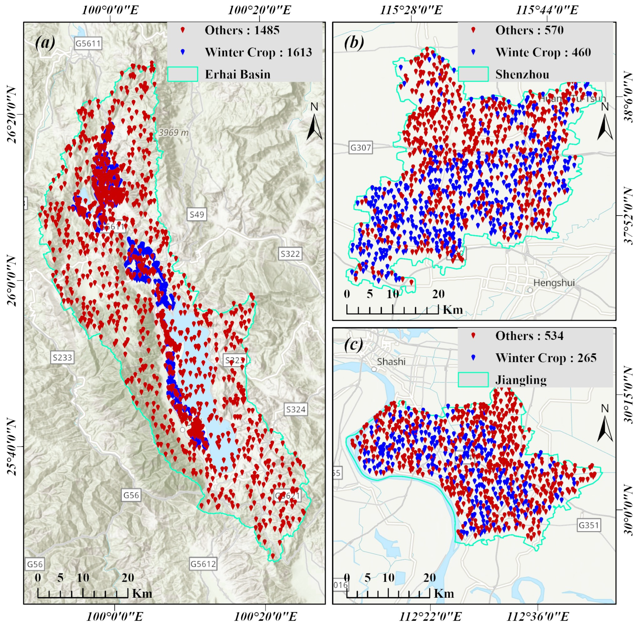
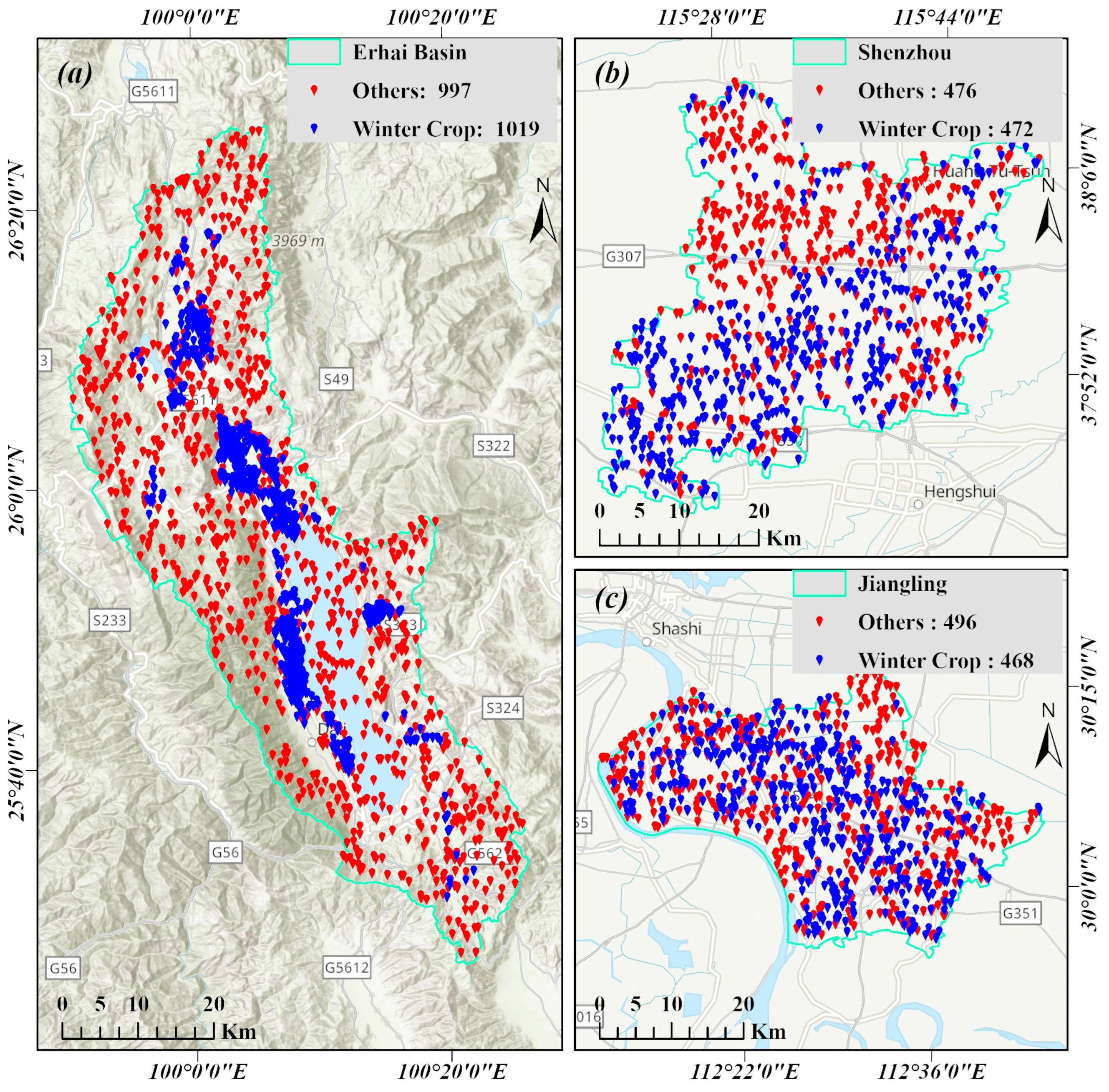
To ensure representativeness and regional diversity, this study selected three typical winter cropping regions across different agroecological zones of China: the Erhai Basin (Figure 1a) in Yunnan Province (Southwest China), Shen City (Figure 1b) in Hebei Province (North China), and Jiangling County (Figure 1c) in Hubei Province (Southeast China). These regions differ significantly in climate, topography, and cropping patterns and together reflect the major types of winter crop cultivation in China. Study area 1 (SA 1) is the Erhai Basin, located on the Yunnan–Guizhou Plateau in Southwestern China. It encompasses parts of Dali City and Eryuan County, with geographic coordinates ranging from 25.60° N to 25.97° N and 100.08° E to 100.28° E, and covers an area of approximately 2565 km2. The region features a subtropical plateau monsoon humid climate, with an average annual temperature of 14.9 °C and mean annual precipitation of 1051.1 mm. The topography is highly variable, with elevations ranging from 1962 m to 4011 m. Farmland in the central basin is situated at around 2000 m elevation. Winter cropping in this area is dominated by lettuce and broad beans, with small areas of winter wheat and winter rapeseed. Sowing typically occurs in October, with harvesting in April of the following year. Study area 2 (SA 2) is Shenzhou City in Hebei Province, located on the North China Plain. It lies between 37.70° N to 38.18° N and 115.35° E to 115.85° E, covering a total area of about 1252 km2. The region has a warm temperate semi-arid monsoon climate, with an average annual temperature of 13.4 °C and annual precipitation of 486 mm. The terrain is flat, gradually sloping from west to east, with elevations ranging from 17.5 m to 28 m. As one of China’s primary winter wheat-producing regions, the dominant winter crop is winter wheat, with the limited cultivation of winter rapeseed. Sowing usually takes place in October, followed by harvesting in June. Study area 3 (SA 3) is Jiangling County in Hubei Province, situated in the Jianghan Plain of Central China. The area spans from 29.90° N to 30.65° N and from 112.73° E to 115.73° E, covering approximately 1048.7 km2. The county has a northern subtropical monsoon humid climate, with an average annual temperature of 16.0 °C and average annual precipitation of about 1000 mm. The terrain is flat, with elevations ranging from 25.3 m to 40.0 m. Winter rapeseed is the predominant winter crop, accompanied by small areas of winter wheat. Similarly to the other regions, sowing occurs around October and harvesting around June.

2.2. Data Source

2.2.1. Sentinel-2 Data

Sentinel-2 is a multispectral Earth observation satellite constellation developed and operated by the European Space Agency (ESA), designed to provide high-resolution imagery for applications such as land cover mapping, vegetation monitoring, and environmental assessment [41]. Sentinel-2 provides multispectral imagery with a 5-day revisit cycle at the equator, offering high temporal resolution for monitoring crop growth [42]. It includes 13 spectral bands from the visible to shortwave infrared range, with four key bands (blue, green, red, and near-infrared) at 10 m resolution and additional red-edge and SWIR bands at 20 m resolution.
In this study, Sentinel-2 imagery was accessed via Google Earth Engine (GEE), a cloud-based geospatial analysis platform that allows for efficient and large-scale remote sensing data processing. To improve data quality by mitigating the effects of clouds and cloud shadows, we employed the “Cloud Score+ S2_HARMONIZED V1” dataset available on GEE. This advanced product provides two cloud-related bands, cs and cs_cdf, both ranging from 0 to 1, where higher values indicate a lower probability of cloud contamination. The cs band is more responsive to haze and cloud edges, while the cs_cdf band is less sensitive to low-amplitude spectral disturbances and topographic shadows, thereby yielding a larger number of reliable pixels. In this work, the cs_cdf band was used for cloud and shadow masking to ensure the quality and continuity of the Sentinel-2 time-series data. In this study, we utilized Sentinel-2 imagery covering the entire growth period of winter crops, from October of the current year to June of the following year. The data year for the Erhai Basin is 2024, while the data year for Shenzhou City and Jiangling County is 2023.
To further evaluate the temporal dynamics of Sentinel-2 data availability, we calculated the average number of valid observations per month for each study area during the winter crop growing season, as shown in Figure 2. Overall, Shenzhou City exhibited the most stable and consistently high observation frequency, with approximately 5-6 cloud-free acquisitions per month, reflecting the relatively dry and clear winter conditions typical of Northern China. In contrast, the Erhai Basin showed substantial monthly variation, peaking in January and February with more than 8 observations but dropping significantly in March and April—likely due to increased cloudiness and mountain-induced atmospheric effects in spring. Jiangling County experienced the lowest number of valid observations, rarely exceeding 3 per month, highlighting the challenges posed by frequent overcast and foggy conditions in the Jianghan Plain.

2.2.2. Crop Sample Data

To support the validation tasks, a comprehensive set of ground samples was collected for each study area, encompassing both winter crops and other land cover types. The spatial distribution of these manually labeled samples is illustrated in Figure 3. In the Erhai Basin (Figure 3a), a total of 3098 samples were acquired, including 1613 winter crop samples and 1485 samples of other land cover types. Winter crop samples in this region were obtained through field surveys, while non-winter crop samples were supplemented via a visual interpretation of high-resolution imagery, in which trained interpreters manually identified crop types and other land covers by examining image features such as patterns, shapes, colors, and spatial context. In Shenzhou City, located in the North China Plain (Figure 3b), 1030 samples were collected—460 for winter crops and 570 for other types—with a relatively uniform spatial distribution across the study area. In Jiangling County, situated in the Jianghan Plain (Figure 3c), 799 samples were collected, including 265 winter crop samples and 534 samples representing other land cover types. The samples in both Shenzhou and Jiangling were primarily acquired through a visual interpretation of high-resolution satellite images. These observations highlight the importance of field sampling for ensuring accurate crop classification. It is important to note that the collected samples in this study were used solely for an independent accuracy assessment of the winter crop mapping results and to generate reference results through supervised classification. The main objective was to evaluate the ability of automatically generated samples to replace manually collected samples for high-precision winter crop mapping.

2.2.3. Other Data

To enhance the reliability of automated sample generation and eliminate interference caused by extreme or anomalous cases, we excluded winter crop samples located in non-cropland areas using an existing land cover product, CLCD [43]. It is a 30 m resolution land cover dataset generated by Landsat data, providing detailed classifications including cropland, forest, grassland, and built-up areas, which makes it particularly useful for refining sample quality in agricultural mapping tasks. We downloaded it from https://www.ncdc.ac.cn/portal/metadata/9de270f3-b5ad-4e19-afc0-2531f3977f2f (accessed on 18 June 2025). The land cover map of the study area can be found in the Supplementary File.

2.3. Methodology

2.3.1. An Overview of the Winter Crop Mapping Framework

The overall winter crop mapping workflow (Figure 4) has three modules: data preprocessing (Sentinel-2 data are processed to surface reflectance, with clouds removed, monthly composites generated, and gaps filled and smoothed; multi-temporal reflectance and vegetation indices were input), sample generation (the WCI from the NDVI time series, the Otsu algorithm for the threshold, coarse classification, random sampling, and a 3 × 3 filter for reliable samples), and supervised classification (RF, SVM, and XGBoost with Bayesian-optimized hyperparameters, validated by ground truth and the best model for the final map determined, evaluated with independent samples); monitored crops include winter wheat, rapeseed, lettuce and broad beans in specific areas.

2.3.2. Sentinel-2 Data Processing

Sentinel-2 data preprocessing for crop classification involved filtering Level 2A images by 80% cloud cover, removing clouds/shadows via Cloud Score+, resampling 20 m bands to 10 m. We used the Cloud Score+ dataset on the GEE platform, which recommends setting the threshold between 0.5 and 0.65 to remove clouds and cloud shadows. Following this recommendation, we set the threshold to 0.6. To construct the time-series images, we followed a three-step process [44]. Firstly, we synthesized monthly Sentinel-2 images using a median composite approach. Its formula is as follows:
Y m e d i a n = M e d i a n y 1 , y 2 , , y n
where [ y 1 , y 2 , , y n ] is n valid observations from Sentinel-2 within one month, and Y m e d i a n is the median of n observations.
Secondly, we filled data gaps by linear interpolation, using a window size of 3 to achieve the complete coverage of the entire time domain. Its formula is as follows:
Y i n t e r p o l a t i o n = y a f t e r y b e f o r e x a f t e r x b e f o r e x n o w x b e f o r e + y b e f o r e
For each invalid pixel, where x n o w is its index in the monthly composite image, and y b e f o r e and y a f t e r are the nearest valid pixel values in the month before and after it, respectively. x b e f o r e and x a f t e r are the corresponding indices. Y i n t e r p o l a t i o n is the final interpolation result.
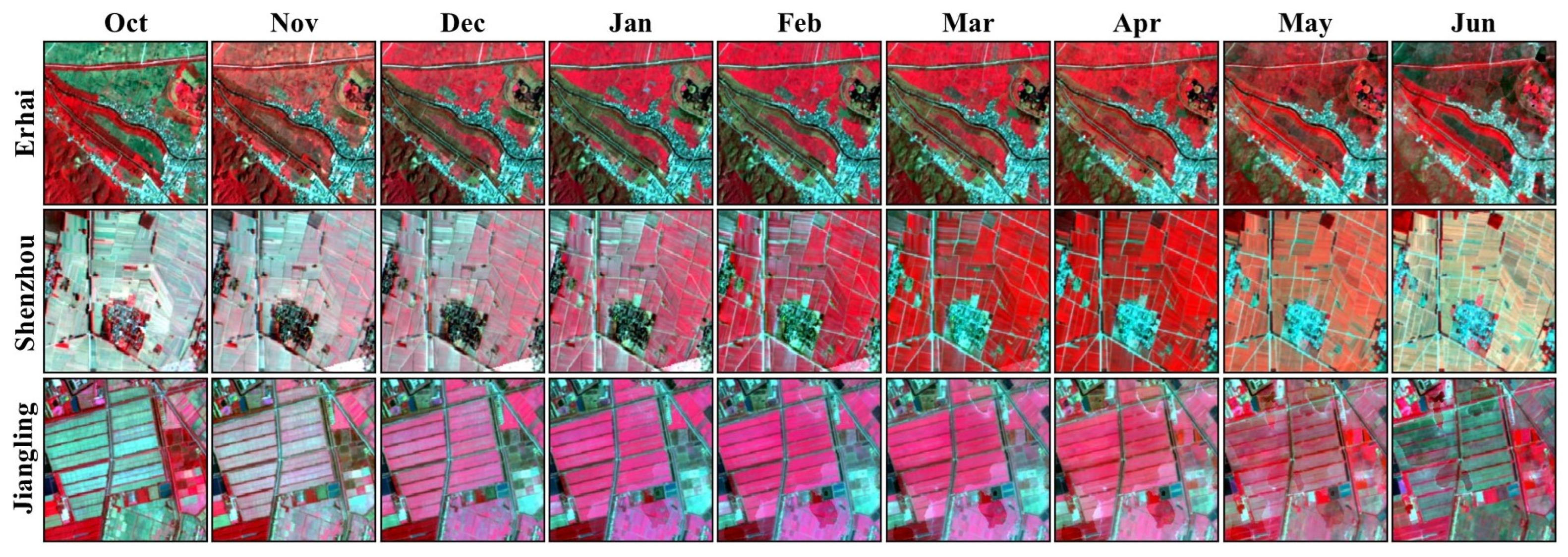
Finally, we applied Whittaker smoothing to smooth the time-series images after interpolation. The Whittaker smoother is a penalized least-squares filter that balances the fit to observed values with temporal smoothness, effectively reducing noise from residual clouds and atmospheric effects [45]. This yielded continuous, cloud-free time-series images (Erhai Basin: Oct–Apr; Shenzhou, Jiangling: Oct–Jun), capturing winter crop phenology (Figure 5). The main crops being monitored were winter wheat and winter rapeseed in the areas of Shenzhou and Jiangling, as well as lettuce and broad beans in the Erhai Lake basin.
To improve the accuracy of crop classification, we calculated four commonly used vegetation indices (Table 1): the Normalized Difference Vegetation Index (NDVI), Enhanced Vegetation Index (EVI), Land Surface Water Index (LSWI), and Green Chlorophyll Vegetation Index (GCVI). These indices provide complementary spectral information that enhances the separability of different crop types.

2.3.3. Generation of Training Samples Based on WCI–Otsu

In this study, we integrated the Winter Crop Index (WCI) with the Otsu algorithm to automatically generate training samples for winter crop mapping [49]. During the winter crop growing season, winter crops exhibit a unique phenological pattern in their NDVI time-series curves that distinguishes them from other land cover types. Vegetation index graphs were compared within each study area between winter crops and non-winter crops, ensuring that the observed patterns were not confounded by differences in crop types between regions. Cross-region comparisons were included only to illustrate general winter crop phenology trends rather than to perform direct quantitative comparisons of index magnitudes. Figure 6 illustrates the NDVI time-series curves of various land cover types across the three study areas.
Overall, winter crops in all three regions show a “decline-then-rise” NDVI curve, with two local minima (sowing and harvest) and one maximum (peak growth). The first minimum is in October; the second and peak times vary by region (Erhai Basin and Jiangling: April, Jan-Feb; Shenzhou: June, April). Fallow lands have low, stable winter NDVI (~0.1) values, rising in summer. Erhai’s forests have high, stable NDVI values; those in Shenzhou and Jiangling vary more, with peaks distinct from crops. Built-up areas and water bodies have consistently low/negative NDVI valueswith little fluctuation. Based on the distinctive NDVI pattern of winter crops, the WCI was calculated as follows:
WCI   =   NDVI max NDVI min 1 × NDVI max NDVI min 2
where NDVImin1 is the NDVI at the sowing stage, NDVImin2 is the NDVI at the harvest stage, and NDVI max is the NDVI at the peak growth stage. Due to differences in crop phenology, region-specific fixed time windows were used to locate NDVImin1, NDVI max , and NDVImin2 for each study area, and the extrema within each window were extracted at the pixel level.
To separate winter crops from other land covers, we applied the Otsu algorithm to determine the optimal WCI threshold [50]. Otsu’s method is a classical global thresholding algorithm widely used in image segmentation. It automatically identifies the threshold that maximizes the between-class variance, effectively separating the image into two classes, foreground (winter crops) and background (other land cover types), without requiring prior knowledge. The between-class variance σ b 2 t is computed as
σ b 2 t =   ω 0 t · ω 1 t · μ 0 t   μ 1 t 2
where t is a candidate threshold, ω 0 ( t ) and ω 1 ( t ) are the proportions of non-winter and winter crop pixels, respectively, and μ 0 ( t ) and μ 1 t are the mean WCI values for each class. The optimal threshold is the value of t that maximizes σ b 2 t , ensuring the best class separability for winter crop identification. The corresponding Otsu-derived thresholds are 0.20, 0.30, and 0.16 for the Erhai Basin, Shenzhou City, and Jiangling County, respectively.
After obtaining the initial winter crop map, we randomly sampled in each study area to obtain the initial training samples. Subsequently, this study uses a spatial filter of a 3 × 3 size in order to retain only those pixels with the same class in the surrounding eight pixels. In this way, easily confused pixels near the boundary are filtered out. The 3 × 3 kernel was selected because it is the smallest neighborhood capable of effectively eliminating mixed boundary pixels while preserving most core-area samples; larger kernels such as 5 × 5 would reduce noise further but also substantially decrease the number of available samples. In addition, the cropland layer from CLCD was employed to suppress potential errors resulting from outlier observations in the derived winter crops.

2.3.4. Bayesian-Optimized Machine Learning Methods

Machine learning algorithms have demonstrated strong potential in crop classification tasks due to their ability to capture complex, non-linear relationships between spectral–temporal features and land cover types [41]. Unlike traditional pixel-based classifiers, machine learning models can incorporate multiple input features and learn discriminative patterns from large labeled datasets. They are also capable of handling noisy or imbalanced data and often require fewer assumptions about the underlying data distributions. In this study, we selected three widely used and representative supervised machine learning algorithms—a Support Vector Machine (SVM), Random Forest (RF), and eXtreme Gradient Boosting (XGBoost)—to evaluate and compare their performance in winter crop classification across multiple study areas.
SVMs are robust and widely adopted classification algorithms that construct an optimal hyperplane to separate different classes in the feature space [51]. They are particularly effective in high-dimensional spaces and in cases where the number of samples is relatively small compared to the number of features. An SVM uses kernel functions to project data into a higher-dimensional space where linear separation is possible. Its strength lies in maximizing the margin between classes, thereby improving generalization performance. Based on its proven performance in previous studies, the kernel function is set to the Radial Basis Function (RBF) [52].
RF is an ensemble learning algorithm that combines the outputs of multiple decision trees to produce more accurate and stable predictions [53]. Each tree in the forest is trained on a random subset of the data with a random subset of features, which introduces diversity and reduces the risk of overfitting. RF is known for its robustness, interpretability, and ability to handle large datasets with noisy or missing values. It also provides variable importance scores, which can help identify key features for crop classification.
XGBoost is a highly efficient implementation of gradient boosting that builds additive tree models in a sequential manner [54]. At each iteration, it attempts to correct the errors made by the previous ensemble by minimizing a differentiable loss function. XGBoost introduces regularization techniques to control model complexity and prevent overfitting, making it well suited for structured classification tasks such as land cover mapping. It also supports parallel and distributed computing, allowing it to process large datasets efficiently.
Optimizing the hyperparameters of machine learning models is crucial for improving classification accuracy and generalization performance, particularly in remote sensing applications where model sensitivity can be high due to complex spectral and temporal features. In this study, we employed Bayesian Optimization (BO) to tune the hyperparameters of machine learning methods. Bayesian optimization, as a very effective global optimization algorithm, requires only a small number of iterations to obtain a desired solution by designing a proper probabilistic agent model and a payoff function [4]. The optimized hyperparameters and the range of values are shown in Table 2.

2.3.5. Accuracy Evaluation

We evaluated the accuracy of crop classification by constructing a confusion matrix. The confusion matrix is currently the most commonly used method for assessing classification accuracy. The following classification metrics were calculated from the confusion matrix: Producer’s Accuracy (PA), User’s Accuracy (UA), Overall Accuracy (OA), F1, and Macro-F1. PA and UA indicate the classification accuracy of individual classes. OA represents the overall classification accuracy. F1-score is a combination of OA and PA. F1-score is a combination of OA and PA. The formulas for these metrics are as follows:
OA = i = 1 n X ii X
PA = X ii X i
U A = X i i X i
F 1 = 2   ×   PA   ×   UA PA + UA
in (5)–(8), n is the total number of categories, and X i i is the row i and the column i value in the confusion matrix, representing the number of pixels of class i that are correctly classified. X represents the total number of test samples. X i is the sum of row i in the confusion matrix, representing the true number of samples of class i. X i is the sum of column i in the confusion matrix, representing the number of samples predicted to be class i.

3. Results

3.1. Training Samples Generated Based on WCI-OSTU

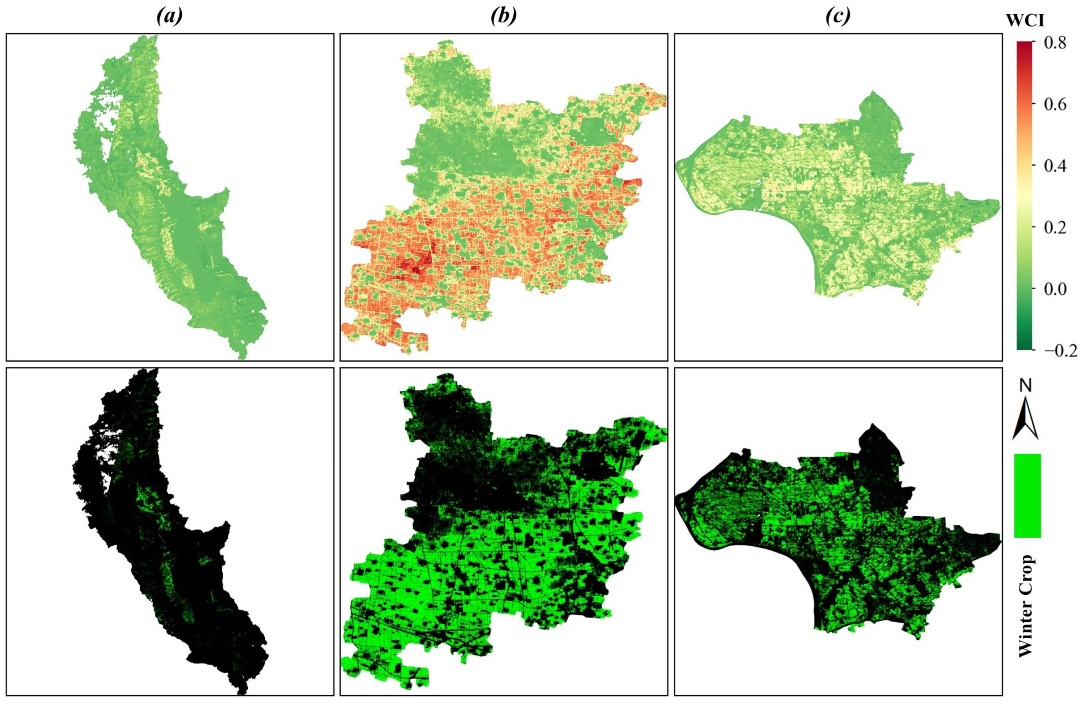
In this study, training samples were generated based on the WCI–Otsu method. First, we calculated the WCI for the three study areas and applied the Otsu algorithm to determine the optimal threshold that distinguishes winter crops from other land cover types. The resulting WCI values and corresponding initial classification maps are shown in Figure 7. The WCI values across the three study areas ranged from −0.2 to 0.8, with the corresponding Otsu-derived thresholds being 0.20, 0.30, and 0.16 for the Erhai Basin, Shenzhou City, and Jiangling County, respectively. The OA values of the corresponding initial classification results are 0.8999, 0.9610 and 0.9456, respectively. It should be noted that due to the influence of clouds, some areas in the initial classification results obtained based on the WCI are missing; therefore, samples falling into the missing areas will not be included in the evaluation. Notably, the WCI values in Shenzhou City were significantly higher than those in the other two regions, resulting in a higher threshold. In contrast, the WCI values in the Erhai Basin and Jiangling County were relatively similar and lower, leading to much lower classification thresholds. This indicates that distinguishing winter crops from other land covers using the WCI–Otsu method is more effective and reliable in Shenzhou City. The classification results based on the Otsu thresholds were generally consistent with the spatial distribution of the WCI, demonstrating clear separation between winter crops and non-winter land covers. However, in the northern part of the Erhai Basin, large areas of missing values were observed due to persistent cloud cover. Given the region’s complex and mountainous terrain, cloud contamination poses a more significant challenge in this area compared to Shenzhou and Jiangling, where such issues are minimal. This factor did not seriously affect the interpretation of cross-region comparisons, as the analyses focused primarily on within-region patterns rather than direct quantitative comparisons between areas. Although errors in identifying NDVImin1 or NDVImin2 can lead to unreliable WCI values, in this study, the WCI was used solely to produce an initial classification from which winter crop samples were extracted. These samples were subsequently used to train a supervised classification model, enabling the refinement of classification results and reducing the influence of potential WCI errors on the final maps.
To better illustrate the spatial details of the WCI values and the corresponding classification results based on the Otsu threshold, one representative area was selected from each study region for visualization. The results are shown in Figure 8. These local visualizations were consistent with the overall trends observed across the full study areas. Region 1, located in the northern part of the Erhai Basin, highlights the issue of extensive missing values due to persistent cloud cover. In farmlands adjacent to mountainous areas, large gaps were observed, where many winter crop fields could not be correctly identified, which was possibly due to the cloudiness present in the satellite images, reducing the number of high-quality observations. In contrast, farmland areas farther from the mountains showed improved classification performance. In this test area, the WCI–Otsu method underestimated the extent of winter crops, with many actual winter crop pixels misclassified as other land cover types, indicating limited effectiveness under such challenging conditions. In Shenzhou City, the WCI values of winter crops were significantly higher than those of other land cover types. Fallow land and built-up areas exhibited similar, low WCI values. In the regions where winter crops were intensively cultivated, the WCI–Otsu method performed exceptionally well, yielding clean classification results with minimal noise. Even narrow mixed pixels caused by field boundaries or roads were accurately distinguished. A small number of scattered winter crops within the fallow areas in the lower-right corner were also correctly identified. Overall, the WCI–Otsu method showed excellent performance in Shenzhou City. In Jiangling County, although the farmland was relatively fragmented and fields were smaller in size, the WCI–Otsu method still effectively differentiated winter crops from other land cover types. It was also able to identify small, isolated winter crop fields. Despite Jiangling and the Erhai Basin both being located in Southern China, differences in cropping patterns and topography contributed to better performance in Jiangling. The relatively simple principle behind the WCI makes it less effective under complex weather conditions and planting structures. In summary, the WCI–Otsu method demonstrated strong capability in most parts of all three study regions, providing an initial and reasonably accurate winter crop classification. These preliminary classification results can serve as a foundation for subsequent training sample generation and supervised classification using machine learning algorithms.
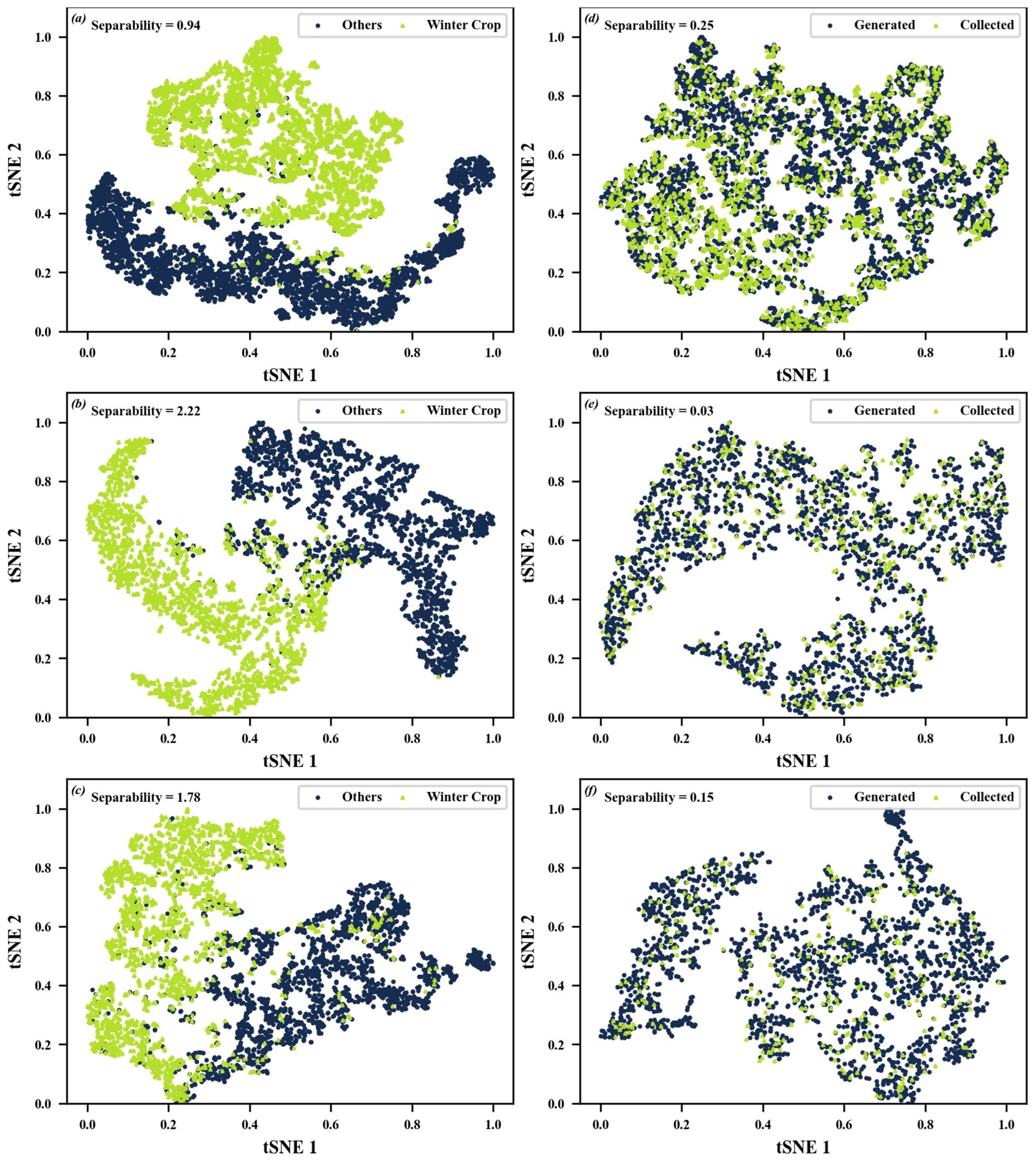
After obtaining the initial crop classification results using the WCI–Otsu method, we performed random sampling within the three study areas to generate initial training samples. Subsequently, a 3 × 3 spatial filter was applied, along with the cropland layer from the CLCD dataset, to eliminate edge pixels and anomalous observations, resulting in a set of reliable training samples. To assess the quality of the generated training samples, we employed t-distributed Stochastic Neighbor Embedding (t-SNE) for dimensionality reduction and visualization. t-SNE is a non-linear technique that projects high-dimensional data into a lower-dimensional space while preserving local structure, making it particularly effective for visualizing complex, non-linear relationships in the data [55]. Figure 9 presents the t-SNE visualization results for both automatically generated and manually collected samples across the three study areas. Figure 9a–c illustrate the feature distribution of winter crops and other land cover types in the generated training samples. These two classes are generally well separated, with clear boundaries in most cases. However, some confusion is observed at the boundaries between classes. In the Erhai Basin, a few non-winter crop samples are mixed with winter crop samples. In Shenzhou City, the samples are relatively pure, with minimal mixing outside boundary regions. In Jiangling County, a slight overlap between the two classes is observed even away from the boundaries. Figure 9d–f compare the generated and manually collected winter crop samples. The two sample sets almost completely overlap in the feature space, indicating high consistency in both distribution and coverage. To quantitatively evaluate the sample quality, we calculated the separability index, defined as the ratio of inter-class distance to the average intra-class variance. A higher ratio indicates better class separability. For the generated training samples, the separability values between winter crops and other land cover types were 0.94, 2.22, and 1.78 for the Erhai Basin, Shenzhou City, and Jiangling County, respectively. The same values were observed for the manually collected samples, indicating strong agreement. In the Erhai Basin, the separability is close to 1 due to complex land cover types, making it more challenging to distinguish winter crops. Crops in areas with rugged topography often exhibit such characteristics due to microclimatic variations, slope-induced differences in soil moisture, and shading effects. In contrast, the higher separability in Shenzhou and Jiangling suggests simpler land cover composition and reduced classification difficulty. Furthermore, the separability between the generated and manually collected winter crop samples was 0.25, 0.03, and 0.15, respectively, across the three regions. These low values indicate strong similarity between the two sets. Overall, the automatically generated samples closely match the manually collected ones, demonstrating that the WCI–Otsu-based sample generation method is feasible and effective for supervised classification.
The spatial distribution and quantity of automatically generated training samples for winter crop mapping are illustrated in Figure 10. In each study area, the training samples are well distributed across the entire region, and the spatial patterns of both winter crop samples and other land cover samples are consistent with the actual land cover distribution. In the Erhai Basin, winter crops are primarily cultivated in the central plains, resulting in a concentration of winter crop samples in that area. In contrast, samples representing other land cover types are mainly located around Erhai Lake and the surrounding mountainous regions. In Shenzhou City and Jiangling County, both classes of samples (winter crops and others) are evenly distributed across the respective study areas. Due to the larger area of the Erhai Basin, approximately 1000 samples were generated for each class. In the relatively smaller regions of Shenzhou and Jiangling, about 500 samples were obtained per class. Within each study area, sample sizes for different classes were kept roughly balanced to avoid bias in model training, although slight variations occurred due to differences in the availability of high-confidence reference data. This balancing was performed independently within each spatial domain. A balanced sample distribution contributes to improving the accuracy and robustness of winter crop mapping.

3.2. Accuracy of Winter Crop Mapping for Different Machine Learning Methods

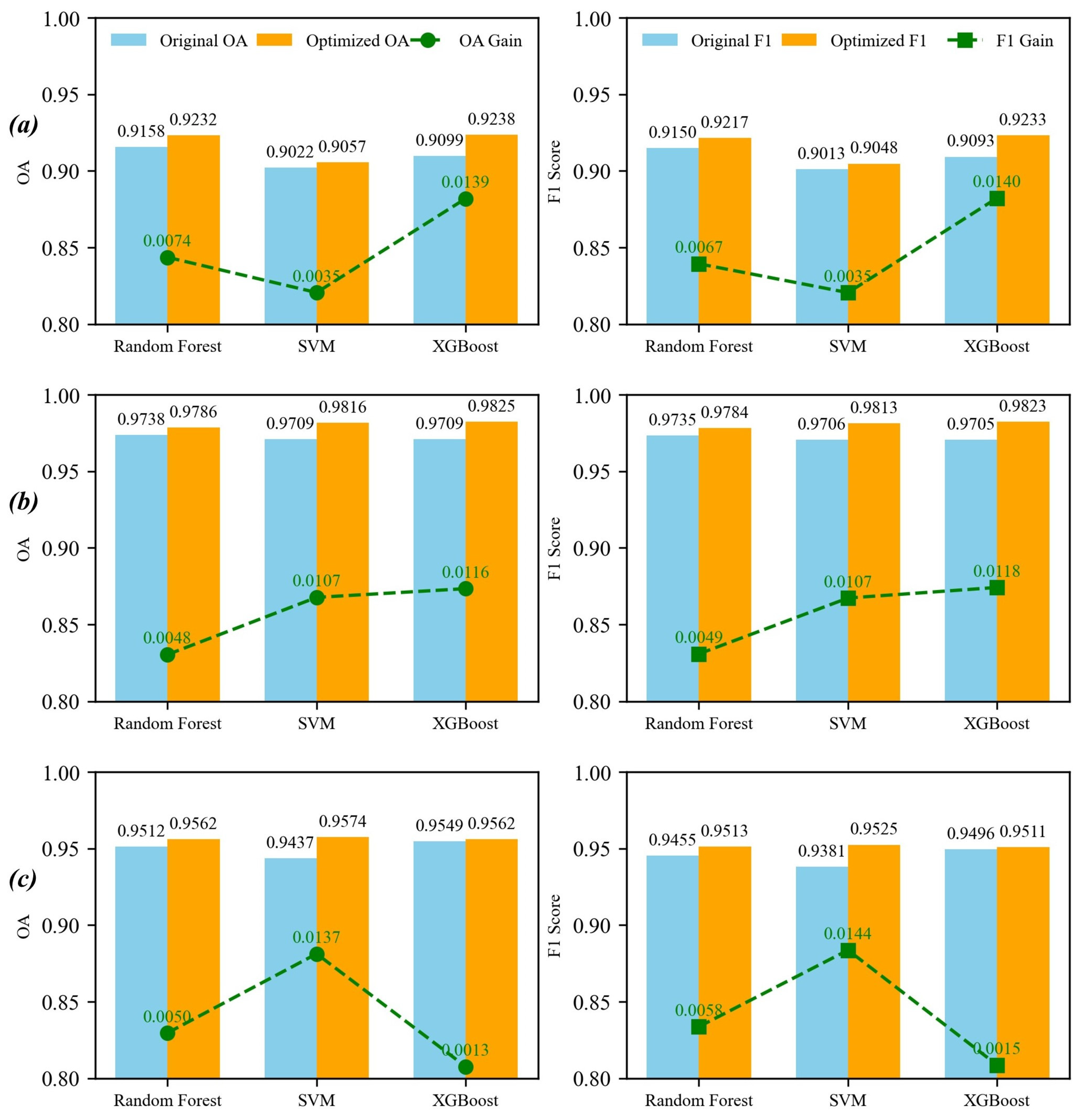
To improve the classification performance of winter crops, model selection and hyperparameter optimization were conducted for three distinct regions: the Erhai Basin, Shenzhou, and Jiangling. The results reveal regional differences in the optimal classification models and their parameter configurations (Table 3). In the Erhai Basin, the XGBoost algorithm was identified as the best-performing model. Compared to the default settings, the optimized model used a smaller number of estimators (reduced from 100 to 74), a shallower tree depth (from 6 to 3), and a significantly lower learning rate (from 1.0 to 0.02). These adjustments effectively reduced model complexity and the risk of overfitting, suggesting that the spectral features in this region have strong separability and benefit from a more conservative learning strategy. For Shenzhou, XGBoost also yielded the best results. The number of estimators increased substantially (from 100 to 191), indicating that a greater ensemble size was necessary to capture complex patterns in the data. Meanwhile, the maximum depth was reduced to 3, and the learning rate was set to 0.60, indicating a trade-off between model capacity and learning stability. The subsample and colsample bytree parameters were also adjusted to enhance the model’s robustness against noise and overfitting. In contrast, Jiangling achieved optimal performance using an SVM model. The penalty parameter, C, was increased from 1.0 to 54.90, placing greater emphasis on minimizing classification error, while gamma was slightly decreased from 0.028 to 0.02 to control the kernel function’s influence. These settings indicate that the SVM benefited from a stronger fitting capability, possibly due to the region’s relatively low feature dimensionality or higher class linear separability. Overall, the results demonstrate the necessity of region-specific model tuning. XGBoost was more effective in regions with complex feature interactions, whereas the SVM outperformed in areas where the feature space was less complex. Hyperparameter optimization significantly improved classification accuracy across all regions, underscoring its critical role in developing high-performance crop mapping models.
Figure 11 presents the confusion matrices for winter crop classification in the three study regions–the Erhai Basin, Shenzhou, and Jiangling–before and after model parameter optimization. The results clearly demonstrate that hyperparameter tuning improves classification performance across different models and regions. In the Erhai Basin, the optimized XGBoost model (BO-XGBoost) outperformed the default configuration by reducing false positives from 203 to 184 and false negatives from 76 to 52. This led to an increase in classification accuracy for winter crops, indicating enhanced model robustness and generalization. For Shenzhou, improvements were also evident. The BO-XGBoost model reduced false positives (13 to 7) and false negatives (17 to 11), further boosting accuracy. Given the already high performance of the default model, the optimization yielded marginal yet meaningful gains in predictive reliability. In Jiangling, the optimized SVM model (BO-SVM) exhibited a trade-off. False positives decreased significantly (from 37 to 22) and false negatives slightly increased (from 8 to 12). This suggests that the optimized model is more conservative in classifying winter crops, potentially minimizing false alarms at the expense of some missed detections. Overall, the results underscore the importance of region-specific model optimization. Bayesian optimization effectively enhances model performance by balancing sensitivity and specificity, particularly in heterogeneous agricultural landscapes.
The classification accuracy of different algorithms is shown in Figure 12. The comparison of classification performance before and after hyperparameter optimization in the Erhai Basin indicates that XGBoost achieved the most significant improvements, with accuracy and the F1-score increasing by 0.0139 and 0.014, respectively. This highlights XGBoost’s sensitivity to parameter tuning and its strong adaptability to complex feature spaces. Random Forest also benefited from optimization, albeit to a lesser extent, suggesting its robustness under default settings. In contrast, the SVM showed minimal improvement, indicating limited sensitivity to parameter changes in this context. Overall, the results emphasize the importance of model-specific optimization strategies to maximize classification accuracy in regional crop mapping tasks. In Shenzhou, the XGBoost model achieved the highest improvement, with accuracy increasing from 0.9709 to 0.9825 and the F1-score rising from 0.9705 to 0.9823. This gain in accuracy and F1 suggests that XGBoost responds well to optimization and is highly effective for crop classification tasks in this region. The SVM also exhibited significant improvement, with both accuracy and the F1-score increasing by 0.107, indicating that careful parameter tuning can substantially enhance the SVM’s performance, even though it is typically considered less flexible than tree-based models. While RF started with the highest baseline accuracy (0.9738), its post-optimization gains were the smallest (only 0.0048 in accuracy and 0.0049 in the F1-score). This suggests that RF performs robustly under default settings but has less room for improvement compared to the other models. In Jiangling, the SVM model achieved the most notable improvement, with accuracy increasing from 0.9437 to 0.9574 and the F1-score from 0.9381 to 0.9525. These gains of 0.0137 in accuracy and 0.0144 in the F1-score suggest that the SVM’s performance is highly sensitive to parameter tuning, and proper optimization can significantly enhance its effectiveness, particularly in scenarios with moderate class separability. The RF model also showed modest improvement, with accuracy increasing by 0.005 and the F1-score by 0.0058. These results indicate that while RF is relatively robust under default settings, targeted optimization can still yield measurable performance benefits. In contrast, XGBoost exhibited only minor improvements (an accuracy gain of 0.0013 and an F1 gain of 0.0015), suggesting that the model already operated near its performance ceiling with the default configuration. This also reflects the model’s strong out-of-the-box performance in the Jiangling region. In summary, while all models benefited from hyperparameter optimization to varying degrees, XGBoost consistently delivered the highest classification performance in the Erhai Basin and Shenzhou, whereas the SVM emerged as the optimal model in Jiangling County, highlighting the importance of region-specific model selection and tuning strategies. This difference may be attributed to the variation in the spectral separability of crops and sample size distribution among the regions. In Jiangling County, the spectral signatures of winter crops were more distinct, favoring the SVM classifier, whereas in the Erhai Basin and Shenzhou City, the more complex spectral–temporal patterns benefited from the boosted decision tree structure of XGBoost.

3.3. Visualization of Winter Crop Mapping Results

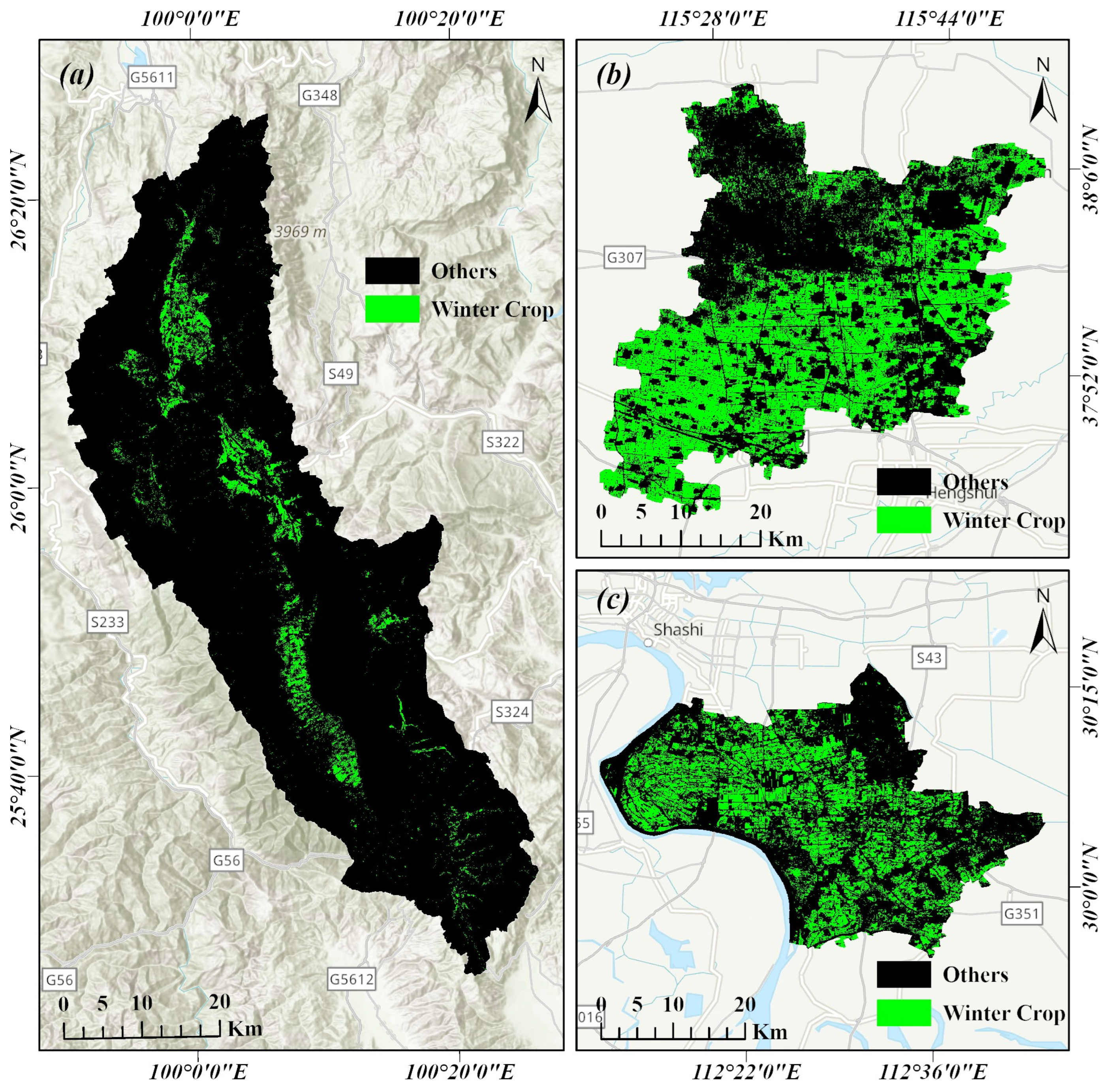
After selecting the optimal model and hyperparameters, we applied the trained model to the entire extent of each study area to generate the final winter crop distribution maps. Figure 13 shows the spatial distribution of winter crops in the three study regions. In the Erhai Basin, winter crops are primarily concentrated in the western and northern plains surrounding Erhai Lake, as well as in Eryuan County. In contrast, the mountainous regions to the east of the lake contain fewer croplands and thus only sparse winter crop presence. A limited number of winter crop fields are also found in the northern part of the basin near the urban area of Dali City. It is worth noting that due to cloud contamination in the northern portion of the Erhai Basin, the WCI–Otsu method failed to fully identify the winter crop areas in this region. Moreover, the WCI–Otsu method relies on only three image acquisition dates, thus utilizing limited temporal information. In contrast, the machine learning models optimized via Bayesian optimization were trained on reconstructed Sentinel-2 time-series data covering the entire crop growth period. These models fully leveraged the phenological dynamics of winter crops, enabling better performance in areas with complex land cover and planting patterns. In addition to filling data gaps, the supervised classification approach improved classification accuracy by capturing temporal variations throughout the growing season. In Shenzhou City, winter crops are mainly distributed in the central and southern regions, while the northern part contains large contiguous areas of fallow land. In Jiangling County, winter crops are uniformly distributed across most of the region, except for some fallow patches in the northeast. Higher mapping efficiency was achieved in Shenzhou City and Jiangling County, whereas in the Erhai Basin, the mapping precision was primarily attained over the intermontane valley where cropland is concentrated. Overall, the proposed method effectively identified winter crop areas across all three regions, demonstrating its robustness and accuracy for large-scale crop mapping.
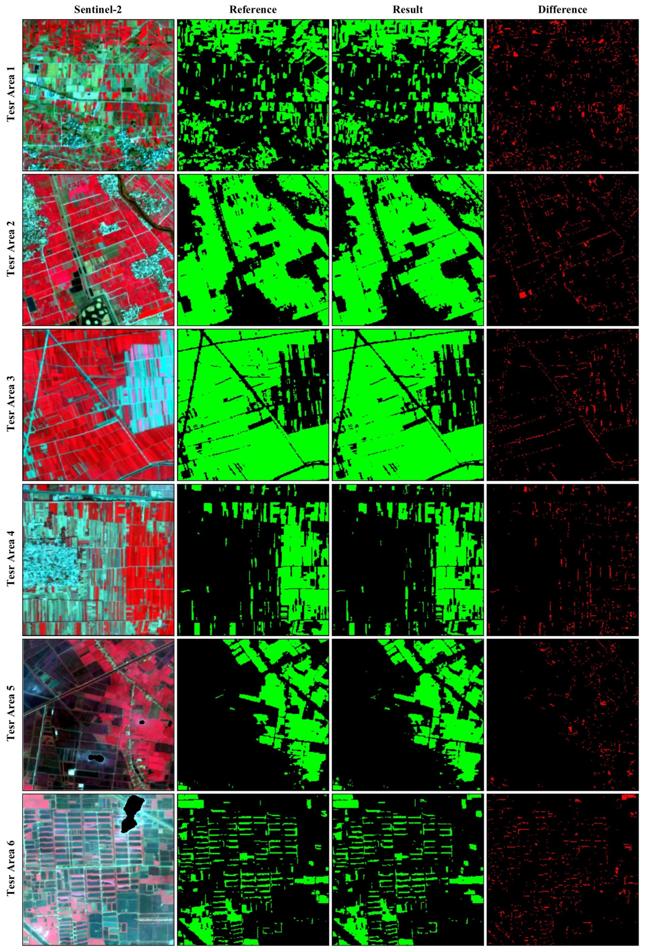
To assess the spatial details of the winter crop mapping results, two local test areas were selected within each study region. As shown in Figure 14, we visualized and compared the winter crop classification results obtained using different methods and quantified the differences between our results and the reference maps. The reference maps were generated using manually collected samples and supervised classification, with the same machine learning models and hyperparameters described previously. Test Areas 1 and 2 are located in the Erhai Basin. In Test Area 1, croplands are highly fragmented, and the field plots are small. A small number of winter crops are scattered within larger fallow areas. Compared with the reference results, our method identified more winter crop regions. In non-vegetated areas, both maps are largely consistent. In Test Area 2, cropland is more concentrated and field sizes are larger, with only limited fallow land. Some non-crop land cover types were misclassified as winter crops. However, our method demonstrated superior performance in delineating narrow field roads compared to the reference. Test Areas 3 and 4 are from Shenzhou City. Test Area 3 features a large expanse of cropland with the minimal presence of other land cover types. A clear boundary is visible between winter crops and fallow land. Most discrepancies between our map and the reference occur within the fallow areas. For linear features such as roads, the reference classification performs slightly better. In contrast, Test Area 4 includes a higher proportion of non-crop land cover, such as fallow land. Our results are largely consistent with the reference, with no significant disagreement observed. Even isolated winter crop parcels were correctly identified. Test Areas 5 and 6 are located in Jiangling County. In Test Area 5, winter crops and other land cover types are nearly equally distributed with clear boundaries. Minor discrepancies are observed in areas with dense winter crop cultivation. Test Area 6 contains many small water bodies and ponds. Sparse winter crops are distributed between them. The classification result closely matches the reference map. To quantitatively evaluate the agreement between our classification and the reference, we calculated the spatial overlap ratio. The overlap ratios for the six test areas are 94.88%, 96.76%, 97.17%, 97.23%, 98.32%, and 96.70%, respectively. The level of agreement is strongly correlated with the complexity of land cover in each test area. Some discrepancies may also arise from differences in class proportions within the training data: in supervised classification, boundary pixels tend to be classified into classes with higher sample proportions. Balanced sampling across classes helps mitigate this bias. In conclusion, our classification results show a high level of consistency with both the reference data and the underlying Sentinel-2 imagery. These findings confirm that the proposed method can achieve high-accuracy, fully automated winter crop mapping without the need for manually collected training samples.

4. Discussion

4.1. Importance Analysis of Crop Classification Features

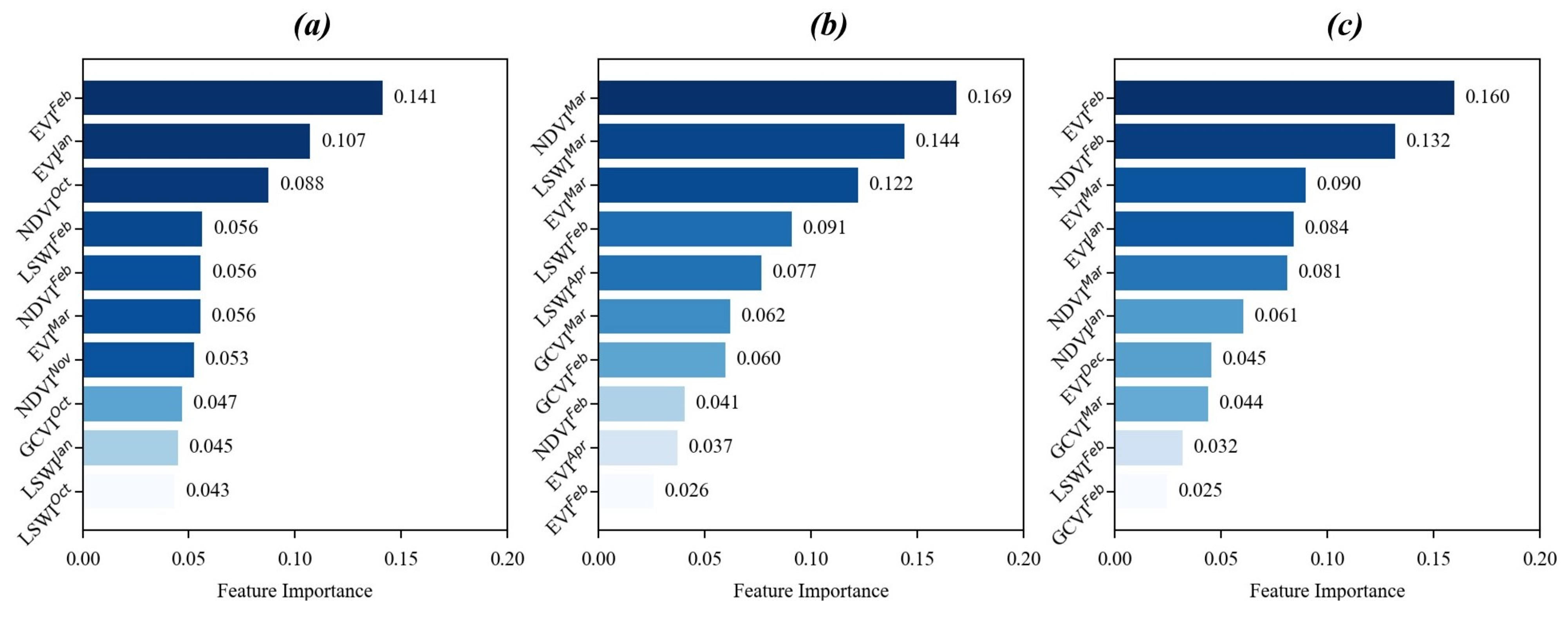
To better understand the contribution of different spectral–temporal features to winter crop classification, a feature importance analysis was conducted based on the RF algorithm. RF not only provides robust classification performance but also yields an intrinsic measure of feature importance by evaluating the decrease in node impurity across all trees [56]. This analysis allows us to identify the most informative vegetation indices and time periods for distinguishing winter crops from other land cover types [57].
As shown in Figure 15, in Erhai, among the top-ranked features, EVIFeb and EVIJan exhibit the highest importance scores, indicating that the vigorous growth of winter crops during mid to late winter provides strong spectral contrast against fallow or non-crop areas. Additionally, the NDVI and GCVI from October and November also show high importance, reflecting their value in capturing early phenological signals such as land preparation or initial crop emergence. The LSWI values from January to February further contribute to classification accuracy by capturing surface moisture conditions, which are typically higher in cultivated winter croplands than in non-crop areas. This increased humidity during the period is primarily attributed to irrigation practices for winter crops, supplemented by occasional rainfall events. These results demonstrate that combining vegetation and moisture indices across key phenological stages allows for the effective characterization of winter crop dynamics in subtropical agricultural systems. In the case of Shenzhou City, the top-ranked features identified by the Random Forest classifier are primarily concentrated in the early spring months, particularly March and February. The most important feature is NDVIMar with an importance score of 0.169, followed by LSWIMar and EVIMar, with scores of 0.144 and 0.122, respectively. These results suggest that March is a critical period for distinguishing winter crops from other land cover types, as vegetation indices in this month capture the greening phase of winter crops. Additionally, multiple features from February (e.g., LSWIFeb, GCVIFeb, NDVIFeb, and EVIFeb) also contribute significantly, indicating that spectral signals during the late winter season are important for early phenological differentiation. Although features from April (e.g., LSWIApr and EVIApr) are included, their relative importance is lower, implying that earlier observations are more discriminative in this region. Overall, the dominance of the NDVI, EVI, LSWI, and GCVI across these months highlights the value of multi-index, multi-temporal features in enhancing classification performance during the critical growth stages of winter crops in Shenzhou. For Jiangling County, the Random Forest model identified February as the most informative period for winter crop classification, with EVIFeb and NDVIFeb being the top two most important features (importance scores of 0.160 and 0.132, respectively). This indicates that the vegetation condition in late winter provides strong discriminatory power for distinguishing winter crops from other land covers. EVIMar and NDVIMar also show high importance, suggesting that early spring phenological signals further enhance classification accuracy. Additionally, EVIJan and NDVIJan contribute notably, highlighting the relevance of pre-spring vegetation dynamics. Interestingly, EVIDec is also included among the top features, implying that spectral characteristics from the previous year can aid in crop identification. The presence of GCVI and LSWI features from February and March, though with lower importance, demonstrates the complementary value of different indices in capturing crop growth patterns. The seasonal trajectories of the NDVI and EVI in our study areas align closely with the phenological development of winter crops. Both indices show low values after sowing, followed by a steady increase during vegetative growth, reaching their peak during heading and grain-filling stages, and then declining sharply at harvest. These temporal patterns are consistent with local crop calendars and field observations. Similarly, the LSWI responds to variations in canopy and soil moisture, often peaking during sowing irrigation or early-season rainfall and declining during senescence or under dry conditions [58]. Such a correspondence between vegetation indices and real-world agronomic processes suggests that these spectral metrics can not only distinguish crop types but also provide valuable insights for crop growth monitoring and agricultural water management [59]. Overall, these results emphasize the critical role of mid-winter to early-spring time-series data in accurately mapping winter crops in subtropical regions like Jiangling.

4.2. Effect of WCI Threshold on Mapping Accuracy

To evaluate the sensitivity of winter crop classification to WCI threshold values, we analyzed the OA and F1-score across a range of thresholds for each study area. Figure 16 presents the classification performance under varying WCI threshold values across the three study areas: Erhai, Shenzhou, and Jiangling. Each curve exhibits a clear peak, indicating the existence of an optimal threshold for distinguishing winter crops from other land cover types. As the threshold increases, classification accuracy first improves and then declines. The yellow dots indicate the WCI thresholds corresponding to the highest OA and F1-score in each region. Vertical dashed lines represent the thresholds automatically determined by the Otsu algorithm. Notably, in all three study areas, the Otsu-derived threshold closely approximates the threshold achieving the best classification accuracy. This demonstrates the effectiveness of the Otsu method in identifying a near-optimal WCI threshold without requiring labeled data. Among the regions, Shenzhou consistently achieved the highest classification accuracy and F1-score across the full range of thresholds, while Erhai Basin showed a comparatively lower performance, possibly due to its more heterogeneous land cover. Overall, the results confirm that combining the WCI with the Otsu algorithm provides a reliable and data-efficient approach for preliminary winter crop classification.

4.3. Advantages, Limitations and Potential Solutions

To address the challenges of large-scale, high-precision winter crop mapping, this study develops a fully automated framework that integrates time-series Sentinel-2 imagery, phenology-driven sample generation, and machine learning classification with Bayesian hyperparameter optimization. The sample generation method based on the WCI–Otsu can automatically generate reliable samples for winter crop mapping. Supervised classification based on time-series images and machine learning can make full use of crop growth information, thereby improving the accuracy of crop classification. The combination of automated sample generation and machine learning algorithms with Bayesian hyperparameter optimization can effectively reduce manual dependence, which is a key path to achieve efficient and automated crop mapping. Using the proposed methodology, long-term winter crop mapping can be conducted at large scales, such as the national level, enabling the continuous monitoring of cropping dynamics. This approach not only identifies the spatial distribution of different winter crops but also detects changes in farmland use, including fallowing, no-till practices, crop rotation, and farmland abandonment [60,61,62]. Such information provides a scientific basis for agricultural authorities to formulate land use policies, optimize cropping structures, assess farmland utilization efficiency, and detect trends or anomalies that may threaten food security in a timely manner [63,64,65]. Long-term crop distribution maps not only reveal the spatial patterns and temporal dynamics of crops but also provide essential baseline data for other agricultural applications, such as crop yield estimation, pest and disease monitoring, and agro-meteorological analysis [66,67]. When integrated with meteorological, soil, and management data, these maps can improve the accuracy of crop models and support agricultural decision-making and risk assessment [68].
Despite the promising results, this study has several limitations. First, it only differentiates winter crops from other land cover types without distinguishing between specific crop species, such as wheat and rapeseed. This may be due to differences in the spectral responses among winter crops, as canopy structure, leaf biochemical composition, and phenological timing can vary substantially even within the same crop category [69]. Incorporating more crop indexes and phenological features could enhance the thematic resolution of the classification [70]. Second, this work only used optical Sentinel-2 imagery, which may be significantly impacted by persistent cloud cover during critical growth stages. Integrating radar data such as Sentinel-1 could mitigate this limitation by providing cloud-penetrating observations [71]. Third, the classification is performed at the pixel level, which may lead to salt-and-pepper noise in heterogeneous landscapes. Incorporating object-based image analysis (OBIA) could improve spatial coherence and classification robustness, particularly in fragmented agricultural regions [72]. Lastly, the current framework is applied to relatively small regions. Future work could leverage cloud computing platforms such as Google Earth Engine (GEE) to scale the approach for large-area winter crop mapping at national or continental levels [73,74].

5. Conclusions

This study proposed an automated winter crop mapping framework that integrates self-generated training samples with Bayesian-optimized machine learning classification. High-quality samples were first derived by combining the WCI with the Otsu algorithm, followed by supervised classification using multi-temporal Sentinel-2 imagery and machine learning models. The experiments conducted across three representative agricultural regions in China—Erhai Basin in Yunnan Province, Shenzhou City in Hebei Province, and Jiangling County in Hunan Province—demonstrated the potential of the proposed method to achieve high-accuracy winter crop mapping without relying on manually collected ground samples in the tested regions and season. The main conclusions are as follows:
  • The WCI effectively distinguishes winter crops from other land cover types. The WCI value ranges vary significantly across regions, with Shenzhou City showing the highest values and the best performance of WCI-based classification.
  • The Otsu algorithm successfully determines optimal WCI thresholds to separate winter crops from other land covers. The combination of the WCI and Otsu enables a reliable initial classification, facilitating the generation of high-quality training samples.
  • Bayesian hyperparameter optimization improves the classification performance, especially for algorithms like XGBoost, which are sensitive to hyperparameter settings. In contrast, RF performs well even with default parameters, while the SVM is less sensitive due to its limited number of tunable hyperparameters.
  • XGBoost yielded the best results in the Erhai Basin and Shenzhou City, while the SVM achieved the highest accuracy in Jiangling County. However, performance differences among the three algorithms were generally small.
Overall, the integration of WCI–Otsu-based sample generation and machine learning classification proves effective for automated, high-precision winter crop mapping. This framework also offers valuable insights for more complex crop type classification tasks in the future.

Supplementary Materials

The following supporting information can be downloaded at: https://www.mdpi.com/article/10.3390/agronomy15092034/s1, Figure S1. Landuse in the Erhai Lake Basin from CLCD; Figure S2. Land use in Shenzhou city from CLCD; Figure S3. Land use in Jiangling county from CLCD.

Author Contributions

F.F.: Conceptualization, Software, Writing—Original Draft; M.G.: Funding Acquisition, Project Administration, Writing—Review and Editing; R.G.: Data Curation, Formal Analysis; Y.J.: Investigation, Writing—Review and Editing; Y.Y.: Resources, Writing—Review and Editing. All authors have read and agreed to the published version of the manuscript.

Funding

This research was funded by the National Key Research and Development Program of China (2021YFD1700400) and State Key Laboratory of Efficient Utilization of Arable Land in Northern China (G2025-05-06).

Institutional Review Board Statement

Not applicable.

Informed Consent Statement

Not applicable.

Data Availability Statement

The data will be available on request.

Conflicts of Interest

The authors declare no conflicts of interest.

References

  1. Zhang, H.; Yuan, H.; Du, W.; Lyu, X. Crop Identification Based on Multi-Temporal Active and Passive Remote Sensing Images. ISPRS Int. J. Geo-Inf. 2022, 11, 388. [Google Scholar] [CrossRef]
  2. Alami Machichi, M.; Mansouri, L.E.; Imani, Y.; Bourja, O.; Lahlou, O.; Zennayi, Y.; Bourzeix, F.; Hanade Houmma, I.; Hadria, R. Crop mapping using supervised machine learning and deep learning: A systematic literature review. Int. J. Remote Sens. 2023, 44, 2717–2753. [Google Scholar] [CrossRef]
  3. Zhang, H.; Zhang, Y.; Liu, K.; Lan, S.; Gao, T.; Li, M. Winter wheat yield prediction using integrated Landsat 8 and Sentinel-2 vegetation index time-series data and machine learning algorithms. Comput. Electron. Agric. 2023, 213, 108250. [Google Scholar] [CrossRef]
  4. Di, Y.; Gao, M.; Feng, F.; Li, Q.; Zhang, H. A New Framework for Winter Wheat Yield Prediction Integrating Deep Learning and Bayesian Optimization. Agronomy 2022, 12, 3194. [Google Scholar] [CrossRef]
  5. Mahlayeye, M.; Darvishzadeh, R.; Nelson, A. Cropping Patterns of Annual Crops: A Remote Sensing Review. Remote Sens. 2022, 14, 2404. [Google Scholar] [CrossRef]
  6. Cheng, Z.; Gu, X.; Du, Y.; Wei, C.; Xu, Y.; Zhou, Z.; Li, W.; Cai, W. Multi-modal fusion and multi-task deep learning for monitoring the growth of film-mulched winter wheat. Precis. Agric. 2024, 25, 1933–1957. [Google Scholar] [CrossRef]
  7. Liu, X.; Zhai, H.; Shen, Y.; Lou, B.; Jiang, C.; Li, T.; Hussain, S.B.; Shen, G. Large-Scale Crop Mapping From Multisource Remote Sensing Images in Google Earth Engine. IEEE J. Sel. Top. Appl. Earth Obs. Remote Sens. 2020, 13, 414–427. [Google Scholar] [CrossRef]
  8. Gallo, I.; Ranghetti, L.; Landro, N.; La Grassa, R.; Boschetti, M. In-season and dynamic crop mapping using 3D convolution neural networks and sentinel-2 time series. ISPRS J. Photogramm. Remote Sens. 2023, 195, 335–352. [Google Scholar] [CrossRef]
  9. Joshi, A.; Pradhan, B.; Gite, S.; Chakraborty, S. Remote-Sensing Data and Deep-Learning Techniques in Crop Mapping and Yield Prediction: A Systematic Review. Remote Sens. 2023, 15, 2014. [Google Scholar] [CrossRef]
  10. Han, Z.; Zhang, C.; Gao, L.; Zeng, Z.; Zhang, B.; Atkinson, P.M. Spatio-temporal multi-level attention crop mapping method using time-series SAR imagery. ISPRS J. Photogramm. Remote Sens. 2023, 206, 293–310. [Google Scholar] [CrossRef]
  11. Niu, B.; Feng, Q.; Chen, B.; Ou, C.; Liu, Y.; Yang, J. HSI-TransUNet: A transformer based semantic segmentation model for crop mapping from UAV hyperspectral imagery. Comput. Electron. Agric. 2022, 201, 107297. [Google Scholar] [CrossRef]
  12. Yu, Q.; Duan, Y.; Wu, Q.; Liu, Y.; Wen, C.; Qian, J.; Song, Q.; Li, W.; Sun, J.; Wu, W. An interactive and iterative method for crop mapping through crowdsourcing optimized field samples. Int. J. Appl. Earth Obs. Geoinf. 2023, 122, 103409. [Google Scholar] [CrossRef]
  13. Hu, Q.; Yin, H.; Friedl, M.A.; You, L.; Li, Z.; Tang, H.; Wu, W. Integrating coarse-resolution images and agricultural statistics to generate sub-pixel crop type maps and reconciled area estimates. Remote Sens. Environ. 2021, 258, 112365. [Google Scholar] [CrossRef]
  14. Qiu, B.; Hu, X.; Chen, C.; Tang, Z.; Yang, P.; Zhu, X.; Yan, C.; Jian, Z. Maps of cropping patterns in China during 2015–2021. Sci. Data 2022, 9, 479. [Google Scholar] [CrossRef]
  15. Tran, K.H.; Zhang, H.K.; McMaine, J.T.; Zhang, X.; Luo, D. 10 m crop type mapping using Sentinel-2 reflectance and 30 m cropland data layer product. Int. J. Appl. Earth Obs. Geoinf. 2022, 107, 102692. [Google Scholar] [CrossRef]
  16. Son, N.-T.; Chi-Farn, C.; Cheng-Ru, C.; Piero, T.; Youg-Sing, C.; Hong-Yuh, G.; Syu, C.-H. A phenological object-based approach for rice crop classification using time-series Sentinel-1 Synthetic Aperture Radar (SAR) data in Taiwan. Int. J. Remote Sens. 2021, 42, 2722–2739. [Google Scholar] [CrossRef]
  17. Tian, H.; Qin, Y.; Niu, Z.; Wang, L.; Ge, S. Summer Maize Mapping by Compositing Time Series Sentinel-1A Imagery Based on Crop Growth Cycles. J. Indian Soc. Remote Sens. 2021, 49, 2863–2874. [Google Scholar] [CrossRef]
  18. He, T.; Li, M.; Jin, D. Deep learning-based time series prediction for precision field crop protection. Front. Plant Sci. 2025, 16, 1575796. [Google Scholar] [CrossRef]
  19. Venkatanaresh, M.; Kullayamma, I. An efficient in-season crop mapping using Sentinel-2 imagery and transformer-based semantic segmentation in Andhra Pradesh, India. Int. J. Remote Sens. 2025, 46, 5149–5170. [Google Scholar] [CrossRef]
  20. Wu, Y.; Peng, Z.; Hu, Y.; Wang, R.; Xu, T. A dual-branch network for crop-type mapping of scattered small agricultural fields in time series remote sensing images. Remote Sens. Environ. 2025, 316, 114497. [Google Scholar] [CrossRef]
  21. Zheng, Y.; Dong, W.; Yang, Z.; Lu, Y.; Zhang, X.; Dong, Y.; Sun, F. A new attention-based deep metric model for crop type mapping in complex agricultural landscapes using multisource remote sensing data. Int. J. Appl. Earth Obs. Geoinf. 2024, 134, 104204. [Google Scholar] [CrossRef]
  22. Khosravi, I. Advancements in crop mapping through remote sensing: A comprehensive review of concept, data sources, and procedures over four decades. Remote Sens. Appl.-Soc. Environ. 2025, 38, 101527. [Google Scholar] [CrossRef]
  23. Singh, G.; Vyas, N.; Dahiya, N.; Singh, S.; Bhati, N.; Sood, V.; Gupta, D.K. A novel pixel-based deep neural network in posterior probability space for the detection of agriculture changes using remote sensing data. Remote Sens. Appl.-Soc. Environ. 2025, 38, 101527. [Google Scholar] [CrossRef]
  24. McCormick, R.; Thenkabail, P.S.; Aneece, I.; Teluguntla, P.; Oliphant, A.J.; Foley, D. Artificial Neural Network Multi-layer Perceptron Models to Classify California’s Crops using Harmonized Landsat Sentinel (HLS) Data. Photogramm. Eng. Remote Sens. 2025, 91, 91–100. [Google Scholar] [CrossRef]
  25. Zhong, L.; Hu, L.; Zhou, H. Deep learning based multi-temporal crop classification. Remote Sens. Environ. 2019, 221, 430–443. [Google Scholar] [CrossRef]
  26. Nguyen, H.T.; Nguyen, L.V.; de Bie, C.A.J.M.; Ciampitti, I.A.; Nguyen, D.A.; Nguyen, M.V.; Nieto, L.; Schwalbert, R.; Nguyen, L.V. Mapping Maize Cropping Patterns in Dak Lak, Vietnam Through MODIS EVI Time Series. Agronomy 2020, 10, 478. [Google Scholar] [CrossRef]
  27. Mishra, D.; Pathak, G.; Singh, B.P.; Mohit; Sihag, P.; Rajeev; Singh, K.; Singh, S. Crop classification by using dual-pol SAR vegetation indices derived from Sentinel-1 SAR-C data. Environ. Monit. Assess. 2022, 195, 115. [Google Scholar] [CrossRef] [PubMed]
  28. Li, H.; Song, X.-P.; Hansen, M.C.; Becker-Reshef, I.; Adusei, B.; Pickering, J.; Wang, L.; Wang, L.; Lin, Z.; Zalles, V.; et al. Development of a 10-m resolution maize and soybean map over China: Matching satellite-based crop classification with sample-based area estimation. Remote Sens. Environ. 2023, 294, 113623. [Google Scholar] [CrossRef]
  29. Kang, X.; Huang, C.; Chen, J.M.; Lv, X.; Wang, J.; Zhong, T.; Wang, H.; Fan, X.; Ma, Y.; Yi, X.; et al. The 10-m cotton maps in Xinjiang, China during 2018–2021. Sci. Data 2023, 10, 688. [Google Scholar] [CrossRef]
  30. Kumari, M.; Varun, P.; Kumar, C.K.; Murthy, C.S. Object-based machine learning approach for soybean mapping using temporal sentinel-1/sentinel-2 data. Geocarto Int. 2022, 37, 6848–6866. [Google Scholar] [CrossRef]
  31. Maleki, S.; Baghdadi, N.; Bazzi, H.; Dantas, C.F.; Ienco, D.; Nasrallah, Y.; Najem, S. Machine Learning-Based Summer Crops Mapping Using Sentinel-1 and Sentinel-2 Images. Remote Sens. 2024, 16, 4548. [Google Scholar] [CrossRef]
  32. Kumar, H.; Kumar, R.; Dutta, S.; Singh, M. Google’s Cloud Computing Platform-Based Performance Assessment of Machine Learning Algorithms for Precisely Maize Crop Mapping Using Integrated Satellite Data of Sentinel-2A/B and Planetscope. J. Indian Soc. Remote Sens. 2023, 51, 2599–2613. [Google Scholar] [CrossRef]
  33. Hamidi, M.; Homayouni, S.; Safari, A.; Hasani, H. Deep learning based crop-type mapping using SAR and optical data fusion. Int. J. Appl. Earth Obs. Geoinf. 2024, 129, 103860. [Google Scholar] [CrossRef]
  34. Lykhovyd, P.; Vozhehova, R.; Bidnyna, I.; Shablia, O.; Averchev, O.; Avercheva, N.; Kozyriev, V.; Marchenko, T.; Leliavska, L.; Haydash, O.; et al. Supervised machine learning in crop recognition through remote sensing: A case study for Ukrainian croplands. Mod. Phytomorphol. 2024, 18, 183–187. [Google Scholar]
  35. Xu, S.; Zhu, X.; Chen, J.; Zhu, X.; Duan, M.; Qiu, B.; Wan, L.; Tan, X.; Xu, Y.N.; Cao, R. A robust index to extract paddy fields in cloudy regions from SAR time series. Remote Sens. Environ. 2023, 285, 113374. [Google Scholar] [CrossRef]
  36. Chen, H.; Li, H.; Liu, Z.; Zhang, C.; Zhang, S.; Atkinson, P.M. A novel Greenness and Water Content Composite Index (GWCCI) for soybean mapping from single remotely sensed multispectral images. Remote Sens. Environ. 2023, 295, 113679. [Google Scholar] [CrossRef]
  37. Xie, Y.; Shi, S.; Xun, L.; Wang, P. A multitemporal index for the automatic identification of winter wheat based on Sentinel-2 imagery time series. Giscience Remote Sens. 2023, 60, 2262833. [Google Scholar] [CrossRef]
  38. Huang, Y.; Qiu, B.; Yang, P.; Wu, W.; Chen, X.; Zhu, X.; Xu, S.; Wang, L.; Dong, Z.; Zhang, J.; et al. National-scale 10 m annual maize maps for China and the contiguous United States using a robust index from Sentinel-2 time series. Comput. Electron. Agric. 2024, 221, 109018. [Google Scholar] [CrossRef]
  39. Wang, M.; Lv, M.; Liu, H.; Li, Q. Mid-Infrared Sheep Segmentation in Highland Pastures Using Multi-Level Region Fusion OTSU Algorithm. Agriculture 2023, 13, 1281. [Google Scholar] [CrossRef]
  40. Shen, Y.; Wang, X.; Zhu, R.; Che, T.; Hao, X. A Downscaling Algorithm for Snow Cover Extent Over the Tibetan Plateau Based on a Similar Conditional Probability and Otsu’s Method. IEEE Trans. Geosci. Remote Sens. 2025, 63, 3543433. [Google Scholar] [CrossRef]
  41. Nabil, M.; Farg, E.; Afify, N.M.; Arafat, S.M. Optimizing crop monitoring: Mapping cultivation stages and types with sentinel-1/2 and random forest algorithm. Int. J. Remote Sens. 2025, 46, 273–299. [Google Scholar] [CrossRef]
  42. Snevajs, H.; Charvat, K.; Onckelet, V.; Kvapil, J.; Zadrazil, F.; Kubickova, H.; Seidlova, J.; Batrlova, I. Crop Detection Using Time Series of Sentinel-2 and Sentinel-1 and Existing Land Parcel Information Systems. Remote Sens. 2022, 14, 1095. [Google Scholar] [CrossRef]
  43. Yang, J.; Huang, X. The 30 m annual land cover dataset and its dynamics in China from 1990 to 2019. Earth Syst. Sci. Data 2021, 13, 3907–3925. [Google Scholar] [CrossRef]
  44. Xuan, F.; Dong, Y.; Li, J.; Li, X.; Su, W.; Huang, X.; Huang, J.; Xie, Z.; Li, Z.; Liu, H.; et al. Mapping crop type in Northeast China during 2013–2021 using automatic sampling and tile-based image classification. Int. J. Appl. Earth Obs. Geoinf. 2023, 117, 103178. [Google Scholar] [CrossRef]
  45. Li, N.; Zhan, P.; Pan, Y.Z.; Zhu, X.F.; Li, M.Y.; Zhang, D.J. Comparison of Remote Sensing Time-Series Smoothing Methods for Grassland Spring Phenology Extraction on the Qinghai-Tibetan Plateau. Remote Sens. 2020, 12, 3383. [Google Scholar] [CrossRef]
  46. Huete, A.R.; Liu, H.Q.; Batchily, K.; van Leeuwen, W. A comparison of vegetation indices global set of TM images for EOS-MODIS. Remote Sens. Environ. 1997, 59, 440–451. [Google Scholar] [CrossRef]
  47. Qin, Y.W.; Xiao, X.M.; Dong, J.W.; Zhou, Y.T.; Zhu, Z.; Zhang, G.L.; Du, G.M.; Jin, C.; Kou, W.L.; Wang, J.; et al. Mapping paddy rice planting area in cold temperate climate region through analysis of time series Landsat 8 (OLI), Landsat 7 (ETM+) and MODIS imagery. Isprs J. Photogramm. Remote Sens. 2015, 105, 220–233. [Google Scholar] [CrossRef]
  48. Zhong, L.H.; Gong, P.; Biging, G.S. Efficient corn and soybean mapping with temporal extendability: A multi-year experiment using Landsat imagery. Remote Sens. Environ. 2014, 140, 1–13. [Google Scholar] [CrossRef]
  49. Yang, G.; Li, X.; Liu, P.; Yao, X.; Zhu, Y.; Cao, W.; Cheng, T. Automated in-season mapping of winter wheat in China with training data generation and model transfer. ISPRS J. Photogramm. Remote Sens. 2023, 202, 422–438. [Google Scholar] [CrossRef]
  50. Otsu, N. A Threshold Selection Method from Gray-Level Histograms. IEEE Trans. Syst. Man Cybern. 1979, 9, 62–66. [Google Scholar] [CrossRef]
  51. Noble, W.S. What is a support vector machine? Nat. Biotechnol. 2006, 24, 1565–1567. [Google Scholar] [CrossRef] [PubMed]
  52. Farmonov, N.; Amankulova, K.; Szatmári, J.; Sharifi, A.; Abbasi-Moghadam, D.; Nejad, S.M.M.; Mucsi, L. Crop Type Classification by DESIS Hyperspectral Imagery and Machine Learning Algorithms. IEEE J. Sel. Top. Appl. Earth Obs. Remote Sens. 2023, 16, 1576–1588. [Google Scholar] [CrossRef]
  53. Breiman, L. Random Forests. Mach. Learn. 2001, 45, 5–32. [Google Scholar] [CrossRef]
  54. Chen, T.; Guestrin, C.; Assoc Comp, M. XGBoost: A Scalable Tree Boosting System. In Proceedings of the KDD’16: 22nd Acm Sigkdd International Conference on Knowledge Discovery and Data Mining, San Francisco, CA, USA, 13–17 August 2016; pp. 785–794. [Google Scholar]
  55. Wang, Y.; Su, H.; Li, M. An Improved Model Based Detection of Urban Impervious Surfaces Using Multiple Features Extracted from ROSIS-3 Hyperspectral Images. Remote Sens. 2019, 11, 136. [Google Scholar] [CrossRef]
  56. Chen, J.; Du, X.; Wang, C.; Cai, C.; Fang, G.; Wang, Z.; Liu, M.; Zhang, H. Zonal Estimation of the Earliest Winter Wheat Identification Time in Shandong Province Considering Phenological and Environmental Factors. Agronomy 2025, 15, 1463. [Google Scholar] [CrossRef]
  57. Liu, M.; He, W.; Zhang, H. CN_Wheat10: A 10 m resolution dataset of spring and winter wheat distribution in China (2018–2024) derived from time-series remote sensing. Earth Syst. Sci. Data Discuss. 2025, 2025, 1–31. [Google Scholar] [CrossRef]
  58. Hou, D.; Chen, J.; Dong, J.; Ji, C.; Feng, J.; Du, G.; Yang, L. A 30-m annual paddy rice dataset in Northeastern China during period 2000–2023. Sci. Data 2025, 12, 1355. [Google Scholar] [CrossRef]
  59. Zhang, H.K.; Shen, Y.; Zhang, X.; Li, J.; Yang, Z.; Xu, Y.; Zhang, C.; Di, L.; Roy, D.P. Robust and timely within-season conterminous United States crop type mapping using Landsat Sentinel-2 time series and the transformer architecture. Remote Sens. Environ. 2025, 329, 114950. [Google Scholar] [CrossRef]
  60. Hu, M.; Tang, H.; Yu, Q.; Wu, W. A new approach for spatial optimization of crop planting structure to balance economic and environmental benefits. Sustain. Prod. Consum. 2025, 53, 109–124. [Google Scholar] [CrossRef]
  61. Li, J.; Yu, W.; Du, J.; Song, K.; Xiang, X.; Liu, H.; Zhang, Y.; Zhang, W.; Zheng, Z.; Wang, Y.; et al. Mapping Maize Tillage Practices over the Songnen Plain in Northeast China Using GEE Cloud Platform. Remote Sens. 2023, 15, 1461. [Google Scholar] [CrossRef]
  62. Xu, S.; Xiao, W.; Yu, C.; Chen, H.; Tan, Y. Mapping Cropland Abandonment in Mountainous Areas in China Using the Google Earth Engine Platform. Remote Sens. 2023, 15, 1145. [Google Scholar] [CrossRef]
  63. He, S.; Shao, H.; Xian, W.; Yin, Z.; You, M.; Zhong, J.; Qi, J. Monitoring Cropland Abandonment in Hilly Areas with Sentinel-1 and Sentinel-2 Timeseries. Remote Sens. 2022, 14, 3806. [Google Scholar] [CrossRef]
  64. Rinaldi, M.; Ruggieri, S.; Ciavarella, F.; De Santis, A.P.; Palmisano, D.; Balenzano, A.; Mattia, F.; Satalino, G. How can be used earth observation data in conservation agriculture monitoring? In Proceedings of the IGARSS 2023—2023 IEEE International Geoscience And Remote Sensing Symposium, Pasadena, CA, USA, 16–21 July 2023; pp. 2022–2025. [Google Scholar]
  65. Zhou, W.; Rao, P.; Jat, M.L.; Singh, B.; Poonia, S.; Bijarniya, D.; Kumar, M.; Singh, L.K.; Schulthess, U.; Singh, R.; et al. Using Sentinel-2 to Track Field-Level Tillage Practices at Regional Scales in Smallholder Systems. Remote Sens. 2021, 13, 5108. [Google Scholar] [CrossRef]
  66. Tian, H.; Wang, P.; Tansey, K.; Wang, J.; Quan, W.; Liu, J. Attention mechanism-based deep learning approach for wheat yield estimation and uncertainty analysis from remotely sensed variables. Agric. For. Meteorol. 2024, 356, 110183. [Google Scholar] [CrossRef]
  67. Das, S.; Biswas, A.; Vimalkumar, C.; Sinha, P. Deep Learning Analysis of Rice Blast Disease Using Remote Sensing Images. IEEE Geosci. Remote Sens. Lett. 2023, 20, 3244324. [Google Scholar] [CrossRef]
  68. Jin, N.; Tao, B.; Ren, W.; He, L.; Zhang, D.; Wang, D.; Yu, Q. Assimilating remote sensing data into a crop model improves winter wheat yield estimation based on regional irrigation data. Agric. Water Manag. 2022, 266, 107583. [Google Scholar] [CrossRef]
  69. Liu, M.; He, W.; Zhang, H. Cross-regional sample generation based on Cropland Data Layer for large-scale winter wheat mapping: A case study of Huang-Huai-Hai Plain, China. Int. J. Appl. Earth Obs. Geoinf. 2025, 142, 104764. [Google Scholar] [CrossRef]
  70. Qiu, B.; Wu, F.; Hu, X.; Yang, P.; Wu, W.; Chen, J.; Chen, X.; He, L.; Joe, B.; Tubiello, F.N.; et al. A robust framework for mapping complex cropping patterns: The first national-scale 10 m map with 10 crops in China using Sentinel 1/2 images. ISPRS J. Photogramm. Remote Sens. 2025, 224, 361–381. [Google Scholar] [CrossRef]
  71. You, N.; Dong, J. Examining earliest identifiable timing of crops using all available Sentinel 1/2 imagery and Google Earth Engine. ISPRS J. Photogramm. Remote Sens. 2020, 161, 109–123. [Google Scholar] [CrossRef]
  72. Vizzari, M.; Lesti, G.; Acharki, S. Crop classification in Google Earth Engine: Leveraging Sentinel-1, Sentinel-2, European CAP data, and object-based machine-learning approaches. GEO-Spat. Inf. Sci. 2024, 28, 815–830. [Google Scholar] [CrossRef]
  73. Latif, R.M.A.; He, J.; Umer, M. Mapping Cropland Extent in Pakistan Using Machine Learning Algorithms on Google Earth Engine Cloud Computing Framework. ISPRS Int. J. Geo-Inf. 2023, 12, 81. [Google Scholar] [CrossRef]
  74. Fernando, W.A.M.; Senanayake, I.P. Developing a two-decadal time-record of rice field maps using Landsat-derived multi-index image collections with a random forest classifier: A Google Earth Engine based approach. Inf. Process. Agric. 2024, 11, 260–275. [Google Scholar] [CrossRef]
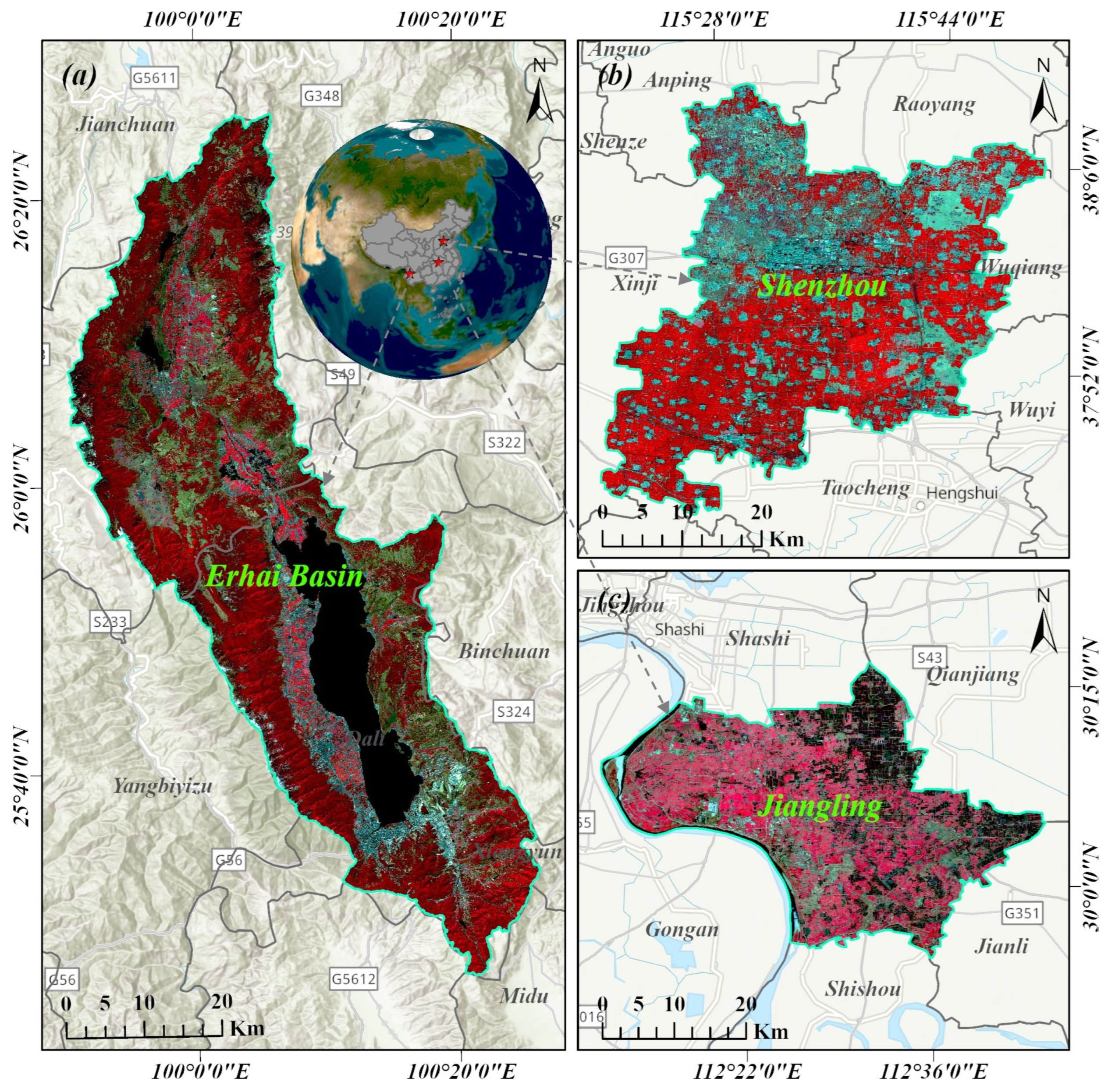
Figure 1. Location of three study areas. (a) the Erhai Basin in Yunnan Province; (b) Shenzhou City in Hebei Province; (c) Jiangling County in Hunan Province.
Agronomy 15 02034 g001
Figure 2. The monthly distribution of valid Sentinel-2 observations in the three study areas.
Agronomy 15 02034 g002
Figure 3. The spatial distribution of manually collected samples for winter crops and other land cover types across the three study areas: (a) Erhai Basin, Yunnan Province; (b) Shenzhou City, Hebei Province; and (c) Jiangling County, Hubei Province.
Agronomy 15 02034 g003
Figure 4. Workflow of winter crop mapping.
Agronomy 15 02034 g004
Figure 5. Phenological variations over agricultural regions are visible from the 10 m monthly Sentinel-2 composites. All panels are shown in the NIR/RED/GREEN band combination.
Agronomy 15 02034 g005
Figure 6. NDVI time-series curves of different land types in the three study areas. (a) the Erhai Basin, Yunnan Province; (b) Shenzhou City, Hebei Province; and (c) Jiangling County, Hubei Province.
Agronomy 15 02034 g006
Figure 7. WCI and corresponding initial classification maps based on Otsu threshold. (a) Erhai Basin, WCI > 0.2; (b) Shenzhou City, WCI > 0.3; and (c) Jiangling County, WCI > 0.16.
Agronomy 15 02034 g007
Figure 8. Local details of WCI and corresponding initial classification maps based on Otsu threshold. (a) Erhai Basin; (b) Shenzhou City; and (c) Jiangling County.
Agronomy 15 02034 g008
Figure 9. t-SNE visualization results of samples from different sources. (ac) winter crops and other land cover types in the generated training samples; (df) the generated and manually collected winter crop samples.
Agronomy 15 02034 g009
Figure 10. The spatial distribution of manually generated samples for winter crops and other land cover types across the three study areas. (a) The Erhai Basin, (b) Shenzhou City, and (c) Jiangling County.
Agronomy 15 02034 g010
Figure 11. Confusion matrix of classification results.
Agronomy 15 02034 g011
Figure 12. Comparison of classification accuracy of different algorithms. (a) The Erhai Basin, (b) Shenzhou City, and (c) Jiangling County.
Agronomy 15 02034 g012
Figure 13. Results of winter crop mapping in the three study areas. (a) The Erhai Basin, (b) Shenzhou City, and (c) Jiangling County.
Agronomy 15 02034 g013
Figure 14. Local details of winter crop maps. Test Area 1 and Test Area 2 are from Erhai Basin. Test Area 3 and Test Area 4 are from Shenzhou City. Test Area 5 and Test Area 6 are from Jiangling County.
Agronomy 15 02034 g014
Figure 15. The top ten classification features of importance for each study area. (a) The Erhai Basin, (b) Shenzhou City, and (c) Jiangling County.
Agronomy 15 02034 g015
Figure 16. Classification accuracy corresponding to different WCI thresholds and Otsu’s threshold.
Agronomy 15 02034 g016
Table 1. The formulation of the four spectral indices used in this study.
IndicesFormulationReference
NDVI N D V I = ρ N I R ρ r e d ρ N I R + ρ r e d [46]
EVI E V I = 2.5 × ρ N I R ρ r e d ρ N I R + 6 × ρ r e d 7.5 × ρ b l u e + 1 [47]
LSWI L S W I = ρ N I R ρ S W I R 1 ρ N I R + ρ S W I R 1 [48]
GCVI G C V I = ρ N I R ρ g r e e n 1   [44]
Table 2. The hyperparameters of machine learning models and their value ranges.
ModelParameterRange
RFn estimators[50, 300]
max depth[5, 50]
min sample split[2, 10]
min sample leaf[1, 10]
max features[1, 56]
SVMC(0.1, 100]
gamma[1 × 10⁻⁵, 1 × 10⁻¹]
XGBoostn estimators[50, 300]
max depth[5, 50]
learning rate[0.1, 1]
subsample[0.5, 1]
colsample bytree[0.5, 1]
Table 3. Hyperparameter optimization results of different algorithms.
RegionBest ModelParameterDefaultOptimized
Erhai BasinXGBoostn estimators10074
max depth63
learning rate1.00.02
subsample0.80.87
colsample bytree0.80.55
ShenzhouXGBoostn estimators100191
max depth63
learning rate1.00.60
subsample0.80.83
colsample bytree0.80.67
JianglingSVMC1.054.90
gamma0.0280.02
Disclaimer/Publisher’s Note: The statements, opinions and data contained in all publications are solely those of the individual author(s) and contributor(s) and not of MDPI and/or the editor(s). MDPI and/or the editor(s) disclaim responsibility for any injury to people or property resulting from any ideas, methods, instructions or products referred to in the content.